advanced spectral methods for climatic time series - Atmospheric ...

More documents

Recommendations

Info

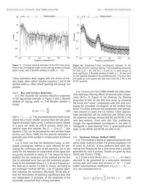
3-18 ● Ghil et al.: CLIMATIC TIME SERIES ANALYSIS 40, 1 / REVIEWS OF GEOPHYSICS Figure 9. Classical spectral estimates of the SOI time series, from a raw correlogram (light curve) and lag-window estimate (bold curve), with a Bartlett window of width m 40. Tukey estimation deals largely with the choice of window shape, often called “window carpentry,” and of the window width m, often called “opening and closing” the window. 3.2.2. Bias and Variance Reduction [117] We illustrate the variance reduction properties of the lag-window estimate in Figure 9 with a Bartlett window of varying width m. The Bartlett window is simply Wmk 1 k , (28) m with k 1, , m. The smoothed estimate (bold curve) clearly has a much smaller variance than the raw periodogram estimate (light curve). Confidence levels relative to a pure red noise, or AR(1) process, which has a spectral slope that behaves like [1 (2f ) 2 ] 1 (see equation (13)), can be calculated for each window shape [Jenkins and Watts, 1968], but the spectral resolution is generally poor if the number N of data points, and hence m, is low. [118] It turns out that the Blackman-Tukey, or windowed correlogram, method is quite efficient for estimating the continuous part of the spectrum, but is less useful for the detection of components of the signal that are purely sinusoidal or nearly so. The reason for this is twofold: the low resolution of this method and the fact that its estimated error bars are still essentially proportional to the estimated mean S˜ X( f ) at each frequency f. We shall see in section 3.4 how to choose, according to the multitaper method (MTM), a set of optimal tapers that maximize the resolution. Moreover, MTM also allows the formulation of statistical significance tests that are independent, in principle, of the amplitude of the sinusoidal component that is being estimated. Figure 10. Blackman-Tukey correlogram estimate of the SSA-filtered SOI’s spectral density. The embedding dimension for SSA is M 60, and RCs 1–4 and 10–11 were chosen as most significant. A Bartlett window of width m 30 was used for the spectral estimate of the prefiltered SOI. The error bars are based on a chi-square test and reach from the 2.5% to the 97.5% quantile. [119] Vautard and Ghil [1989] showed the (data-adaptive) band-pass filtering effects of reconstructed components (RCs). In Figure 10 we illustrate the filtering properties of SSA on the SOI time series by removing the trend and “noise” components with SSA and computing the smoothed correlogram of the residual time series. This filter enhances the components with periodicities around 3.5 years and 5.6 months. These approximate periodicities will be confirmed and refined using the maximum entropy method (MEM) and MTM in the next two sections. Even with this SSA prefiltering, though, the lag-windowed correlogram is not able to distinguish a quasi-biennial from a quasi-quadrennial peak, as the MEM and MTM are able to do. 3.3. Maximum Entropy Method (MEM) [120] This method is based on approximating the time series under study by a linear AR process (equation (1)) of order M, AR(M). It thus performs best when estimating line frequencies for a time series that is actually generated by such a process. Details are given by Burg [1967] and Childers [1978]. [121] Given a time series {X(t)t 1, , N } that is assumed to be generated by a wide-sense stationary process with zero mean and variance 2 , M 1 estimated autocovariance coefficients {ˆ X( j)j 0, , M} are computed from it: Nj 1 ˆ X j Xt Xt j. (29) N 1 j t1
40, 1 / REVIEWS OF GEOPHYSICS Ghil et al.: CLIMATIC TIME SERIES ANALYSIS ● 3-19 Figure 11. Spectral estimates of the SOI time series by the maximum entropy method (MEM). The autocorrelation orders are M 10, 20, and 40 (light, bold, and dashed curves, respectively). The Akaike information content (AIC) criterion [Haykin and Kessler, 1983] predicts an order of M 10, which is obviously too low. In the absence of prior knowledge about the process that generates the time series X(t), M is arbitrary and has to be optimized. The purpose of evaluating (29) is to determine the spectral density Sˆ X that is associated with the most random, or least predictable, process that has the same autocovariance coefficients ˆ. In terms of information theory [Shannon, 1949], this corresponds to the concept of maximal entropy, hence the name of the method. [122] In practice, one obtains estimates {â jj 0, , M} of the regression coefficients a jj 0, , M} from the time series X(t) by assuming that the latter is generated by an AR(M) process and that its order M equals M. The autocorrelation coefficients ˆ X( j) are computed according to (29) and used to form the same Toeplitz matrix C X as in SSA [Vautard and Ghil, 1989; Penland et al., 1991; Vautard et al., 1992]. This matrix is then inverted using standard numerical schemes [Press et al., 1988] to yield the estimated {â j}. The spectral density S X of the true AR process with coefficients {a jj 0 , M} is given by S X f M 1 j1 a 0 aje 2ijf 2 , (30) where a 0 2 is the variance of the residual noise in (1). Therefore the knowledge of the coefficients {â jj 0, , M}, determined from the time series X(t), also yields an estimate Sˆ X of the power spectrum. [123] An example of MEM estimates is given for the SOI time series in Figure 11, using a number of lags M 10, 20, and 40. It is clear that the number of peaks Figure 12. MEM analysis of the SOI time series after SSA prefiltering. The autoregression order used is M 20. The SSA window width is M 60, and RCs 1–4 and 10–11 were chosen, as in Figure 10. increases with M. Two distinct interannual peaks appear only for M 40. This separation between a quasi-biennial and a low-frequency peak is accompanied, unfortunately, by many spurious peaks at higher frequencies. [124] In general, if the time series is not stationary or otherwise not well approximated by an AR process (e.g., if it is generated by nonlinear dynamics), it is necessary to exercise great care in applying MEM. In such cases, cross testing with the application of other techniques is especially important. [125] As the number of peaks in a MEM spectrum increases with M, regardless of the spectral content of the time series, an upper bound for M is generally taken as N/ 2. Heuristic criteria have been devised to refine the choice of a reasonable M [Haykin and Kessler, 1983; Benoist, 1986], based on minimizing the residual of a least squares fit between the AR approximation and the original time series [Akaike, 1969, 1974; Haykin and Kessler, 1983]. Such “information-content” criteria, however, often tend to either underestimate [Benoist, 1986] or overestimate [Penland et al., 1991] the order of regression of a time series, depending on its intrinsic characteristics. [126] The effects of the S/N enhancement performed by SSA decomposition (see section 2) on MEM analysis are illustrated in Figure 12, where the noise components identified by SSA were filtered out prior to MEM analysis. In this example, the power spectrum is much smoother than in Figure 11. The regression order M 20 suffices to separate a quasi-biennial peak at about 2.4 years from a quasi-quadrennial peak at roughly 4.8 years, while no spurious peaks appear at high frequencies. By contrast, Blackman-Tukey spectra of the same time series (see Figure 10 and Rasmusson et al. [1990])
Page 1 and 2: ADVANCED SPECTRAL METHODS FOR CLIMA
Page 3 and 4: 40, 1 / REVIEWS OF GEOPHYSICS Ghil
Page 17: 40, 1 / REVIEWS OF GEOPHYSICS Ghil
Page 41: 40, 1 / REVIEWS OF GEOPHYSICS Ghil

advanced spectral methods for climatic time series - Atmospheric ...

Create successful ePaper yourself

Delete template?

Save as template?