advanced spectral methods for climatic time series - Atmospheric ...

3-8 ● Ghil et al.: CLIMATIC TIME SERIES ANALYSIS 40, 1 / REVIEWS OF GEOPHYSICS
C X k k k. (7)
The eigenvalue k equals the partial variance in the
direction k, and the sum of the k, i.e., the trace of C X,
gives the total variance of the original time series X(t).
[42] An equivalent formulation of (7), which will
prove useful further on, is given by forming the M M
matrix E X that has the eigenvectors k as its columns and
the diagonal matrix X whose elements are the eigenvalues
k, in decreasing order:
E X t CXE X X; (8)
t
here EX is the transpose of EX. Each eigenvalue k gives
the degree of extension, and hence the variance, of the
time series in the direction of the orthogonal eigenvector
k. [43] A slightly different approach to computing the
eigenelements of CX was originally proposed by Broomhead
and King [1986a]. They constructed the N M
trajectory matrix D that has the N augmented vectors
X˜(t) as its rows and used singular-value decomposition
(SVD) [see, for instance, Golub and Van Loan, 1996] of
C X 1
N Dt D (9)
to obtain the square roots of k. The latter are called the
singular values of D and have given SSA its name.
[44] Allen and Smith [1996] and Ghil and Taricco
[1997] have discussed the similarities and differences
between the approaches of Broomhead and King [1986a]
and Vautard and Ghil [1989] in computing the eigenelements
associated in SSA with a given time series X(t).
Both the Toeplitz estimate (6) and the SVD estimate (9)
lead to a symmetric covariance matrix C X. In addition,
the eigenvectors k of a Toeplitz matrix are necessarily
odd and even, like the sines and cosines of classical
Fourier analysis. The Toeplitz approach has the advantage
of better noise reduction when applied to short time
series, as compared with the SVD approach. This advantage
comes at the price of a slightly larger bias when
the time series is strongly nonstationary over the interval
of observation 1 t N [Allen, 1992]. Such biasversus-variance
trade-offs are common in estimation
problems.
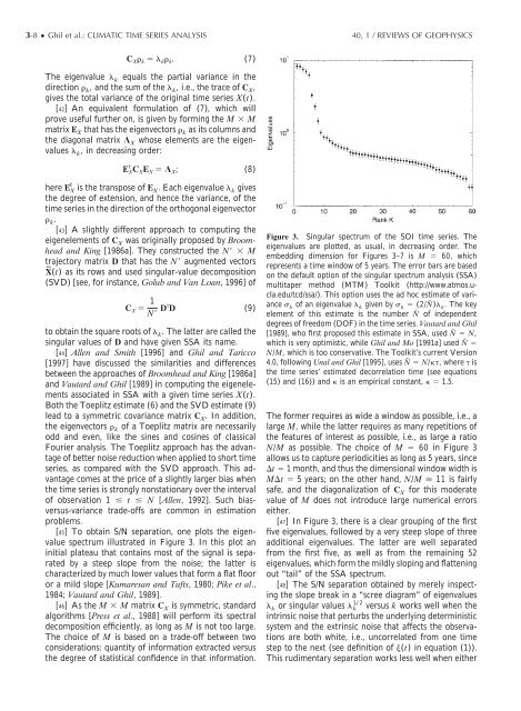
[45] To obtain S/N separation, one plots the eigenvalue
spectrum illustrated in Figure 3. In this plot an
initial plateau that contains most of the signal is separated
by a steep slope from the noise; the latter is
characterized by much lower values that form a flat floor
or a mild slope [Kumaresan and Tufts, 1980; Pike et al.,
1984; Vautard and Ghil, 1989].
[46] As the M M matrix C X is symmetric, standard
algorithms [Press et al., 1988] will perform its spectral
decomposition efficiently, as long as M is not too large.
The choice of M is based on a trade-off between two
considerations: quantity of information extracted versus
the degree of statistical confidence in that information.
Figure 3. Singular spectrum of the SOI time series. The
eigenvalues are plotted, as usual, in decreasing order. The
embedding dimension for Figures 3–7 is M 60, which
represents a time window of 5 years. The error bars are based
on the default option of the singular spectrum analysis (SSA)
multitaper method (MTM) Toolkit (http://www.atmos.ucla.edu/tcd/ssa/).
This option uses the ad hoc estimate of variance
k of an eigenvalue k given by k (2/Nˆ ) k. The key
element of this estimate is the number Nˆ of independent
degrees of freedom (DOF) in the time series. Vautard and Ghil
[1989], who first proposed this estimate in SSA, used Nˆ N,
which is very optimistic, while Ghil and Mo [1991a] used Nˆ
N/M, which is too conservative. The Toolkit’s current Version
4.0, following Unal and Ghil [1995], uses Nˆ N/, where is
the time series’ estimated decorrelation time (see equations
(15) and (16)) and is an empirical constant, 1.5.
The former requires as wide a window as possible, i.e., a
large M, while the latter requires as many repetitions of
the features of interest as possible, i.e., as large a ratio
N/M as possible. The choice of M 60 in Figure 3
allows us to capture periodicities as long as 5 years, since
t 1 month, and thus the dimensional window width is
Mt 5 years; on the other hand, N/M 11 is fairly
safe, and the diagonalization of C X for this moderate
value of M does not introduce large numerical errors
either.
[47] In Figure 3, there is a clear grouping of the first
five eigenvalues, followed by a very steep slope of three
additional eigenvalues. The latter are well separated
from the first five, as well as from the remaining 52
eigenvalues, which form the mildly sloping and flattening
out “tail” of the SSA spectrum.
[48] The S/N separation obtained by merely inspecting
the slope break in a “scree diagram” of eigenvalues
k or singular values k 1/2 versus k works well when the
intrinsic noise that perturbs the underlying deterministic
system and the extrinsic noise that affects the observations
are both white, i.e., uncorrelated from one time
step to the next (see definition of (t) in equation (1)).
This rudimentary separation works less well when either