advanced spectral methods for climatic time series - Atmospheric ...

40, 1 / REVIEWS OF GEOPHYSICS Ghil et al.: CLIMATIC TIME SERIES ANALYSIS ● 3-19
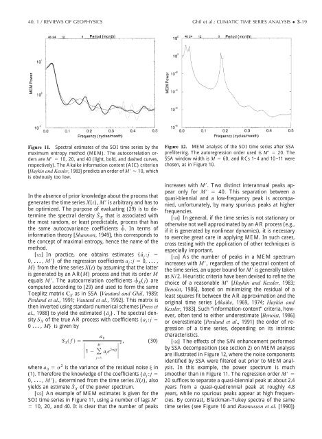
Figure 11. Spectral estimates of the SOI time series by the
maximum entropy method (MEM). The autocorrelation orders
are M 10, 20, and 40 (light, bold, and dashed curves,
respectively). The Akaike information content (AIC) criterion
[Haykin and Kessler, 1983] predicts an order of M 10, which
is obviously too low.
In the absence of prior knowledge about the process that
generates the time series X(t), M is arbitrary and has to
be optimized. The purpose of evaluating (29) is to determine
the spectral density Sˆ X that is associated with
the most random, or least predictable, process that has
the same autocovariance coefficients ˆ. In terms of
information theory [Shannon, 1949], this corresponds to
the concept of maximal entropy, hence the name of the
method.
[122] In practice, one obtains estimates {â jj
0, , M} of the regression coefficients a jj 0, ,
M} from the time series X(t) by assuming that the latter
is generated by an AR(M) process and that its order M
equals M. The autocorrelation coefficients ˆ X( j) are
computed according to (29) and used to form the same
Toeplitz matrix C X as in SSA [Vautard and Ghil, 1989;
Penland et al., 1991; Vautard et al., 1992]. This matrix is
then inverted using standard numerical schemes [Press et
al., 1988] to yield the estimated {â j}. The spectral density
S X of the true AR process with coefficients {a jj
0 , M} is given by
S X f
M
1 j1
a 0
aje 2ijf
2 , (30)
where a 0 2 is the variance of the residual noise in
(1). Therefore the knowledge of the coefficients {â jj
0, , M}, determined from the time series X(t), also
yields an estimate Sˆ X of the power spectrum.
[123] An example of MEM estimates is given for the
SOI time series in Figure 11, using a number of lags M
10, 20, and 40. It is clear that the number of peaks
Figure 12. MEM analysis of the SOI time series after SSA
prefiltering. The autoregression order used is M 20. The
SSA window width is M 60, and RCs 1–4 and 10–11 were
chosen, as in Figure 10.
increases with M. Two distinct interannual peaks appear
only for M 40. This separation between a
quasi-biennial and a low-frequency peak is accompanied,
unfortunately, by many spurious peaks at higher
frequencies.
[124] In general, if the time series is not stationary or
otherwise not well approximated by an AR process (e.g.,
if it is generated by nonlinear dynamics), it is necessary
to exercise great care in applying MEM. In such cases,
cross testing with the application of other techniques is
especially important.
[125] As the number of peaks in a MEM spectrum
increases with M, regardless of the spectral content of
the time series, an upper bound for M is generally taken
as N/ 2. Heuristic criteria have been devised to refine the
choice of a reasonable M [Haykin and Kessler, 1983;
Benoist, 1986], based on minimizing the residual of a
least squares fit between the AR approximation and the
original time series [Akaike, 1969, 1974; Haykin and
Kessler, 1983]. Such “information-content” criteria, however,
often tend to either underestimate [Benoist, 1986]
or overestimate [Penland et al., 1991] the order of regression
of a time series, depending on its intrinsic
characteristics.
[126] The effects of the S/N enhancement performed
by SSA decomposition (see section 2) on MEM analysis
are illustrated in Figure 12, where the noise components
identified by SSA were filtered out prior to MEM analysis.
In this example, the power spectrum is much
smoother than in Figure 11. The regression order M
20 suffices to separate a quasi-biennial peak at about 2.4
years from a quasi-quadrennial peak at roughly 4.8
years, while no spurious peaks appear at high frequencies.
By contrast, Blackman-Tukey spectra of the same
time series (see Figure 10 and Rasmusson et al. [1990])