tsunami inundation maps of whittier and western passage canal ...

More documents

Recommendations

Info

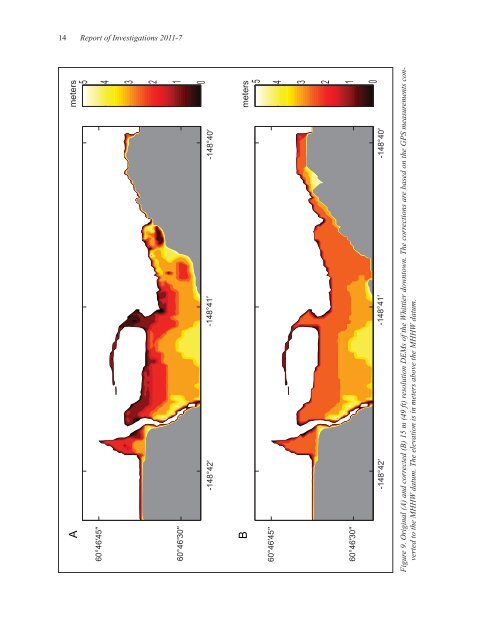
14 Report of Investigations 2011-7 meters A 5 4 3 2 1 0 meters B 5 4 3 2 1 0 Figure 9. Original (A) and corrected (B) 15 m (49 ft) resolution DEMs of the Whittier downtown. The corrections are based on the GPS measurements converted to the MHHW datum. The elevation is in meters above the MHHW datum.
enchmarking. The second component is model verifi - cation, or testing the model, using observations of real events through fi eld data benchmarking. The numerical model that is currently used by the Alaska Earthquake Information Center (AEIC) for tsunami inundation mapping has been validated through a set of analytical benchmarks, and tested against laboratory and fi eld data (Nicolsky and others, 2011). The model solves nonlinear shallow water equations using a fi nite-difference method on a staggered grid. For any coarse–fi ne pair of computational grids, we apply a time explicit numerical scheme as follows. First, we compute the water fl ux within a coarse-resolution grid. These calculated fl ux values are used to defi ne the water fl ux on a boundary of the fi ne-resolution grid. Next, the water level and then the water fl ux are calculated over the fi ne-resolution grid. Finally, the water level computed in the fi ne-resolution grid is used to defi ne the water level within the area of the coarse-resolution grid that coincides with the fi ne grid. Despite the fact that nested grids decrease the total number of grid cells needed to preserve computational accuracy within certain regions of interest, actual simulations are still unrealistic if parallel computing is not implemented. Here, we use the Portable Extensible Toolkit for Scientifi c computation (PETSc), which provides sets of tools for the parallel numerical solution of shallow water equations. In particular, each computational grid listed in table 1 can be subdivided among an arbitrary number of processors. The above-mentioned passing of information between the water fl ux and level is implemented effi ciently using PETSc subroutines. We assess hazards related to tectonic and landslidegenerated tsunamis in Passage Canal by performing model simulations for each hypothetical earthquake and landslide source scenario. In the output of the numerical model, each of the grid points has either a value of 0 if no inundation occurs or 1 if seawater reaches the grid point at any time. The inundation line approximately follows the 0.5 contour between these 0- and 1-point values but was adjusted visually to accommodate obstacles or local variations in topography not represented by the DEM. Although the developed algorithm has passed through the rigorous benchmarking procedures (Nicolsky and others, 2011), the uncertainty in a location of the inundation line is still present. However, this uncertainty is to a greater degree unknown because the inundation line is the result of a complex modeling process. Affecting the accuracy of the inundation line are many factors on which the model depends, including suitability of the earthquake source model, accuracy of the bathymetric and topographic data, and the adequacy of the numerical model in representing the generation, propagation, and runup of tsunami waves. In this report, we do not attempt Tsunami inundation maps of Whittier and western Passage Canal, Alaska 15 to adjust the modeled inundation limits to account for these uncertainty factors. We note that there are several limitations of the model. One of importance is that it does not take into account the periodic change of sea level due to tides. We conducted all model runs using bathymetric data that correspond to MHHW, with the exception of numerical modeling of the 1964 tsunami for the purpose of model validation. The 1964 runs were conducted using the stage of tide at the time of the earthquake, approximately Mean Low Water. For the generation mechanism, we modeled earthquakes and landslides as potential sources of tsunami waves. In this region, it was important to include landslide tsunami sources because underwater landslides and their resultant tsunamis caused a signifi cant portion of the damage in Passage Canal during the 1964 Great Alaska Earthquake. NUMERICAL MODEL OF LANDSLIDE- GENERATED TSUNAMI WAVES To simulate tsunami waves produced by multiple underwater slope failures in Passage Canal on March 27, 1964, we used a numerical model of a viscous underwater slide with full interactions between the deforming slide and the water waves that it generates. This model was initially proposed by Jiang and LeBlond (1992). Fine and others (1998) improved the model by including realistic bathymetry, and by correcting errors in the governing equations. The Fine model’s assumptions and applicability to simulating underwater mudfl ows are discussed by Jiang and LeBlond (1992, 1994) in their formulation of the viscous slide model. The model uses long-wave approximation for water waves and the deforming slide, which means that the wavelength is much greater than the local water depth, and the slide thickness is much smaller than the characteristic length of the slide along the slope (Jiang and LeBlond, 1994). Assier-Rzadkiewicz and others (1997) argued that the long-wave approximation could be inaccurate for steeper slopes exceeding 10 degrees. Rabinovich and others (2003) studied the validity of the long-wave approximation for slopes greater than 10 degrees and found that for a slope of 16 degrees, the possible error was 8 percent, and for the maximum slope in their study of 23 degrees, the possible error was 15 percent. Since the average pre-earthquake offshore slopes from 10 to 30 degrees in the vicinity of Whittier, the possible error introduced by a slide moving down these higher gradient slopes could be signifi cantly higher, and further scientifi c studies are necessary. The advantage of the vertically integrated model by Jiang and LeBlond (1992) is its ability to simulate runup of real landslide tsunami events using high-resolution numerical grids. Although model runs require the use
Page 1: Report of Investigations 2011-7 Ver
Page 4 and 5: STATE OF ALASKA Sean Parnell, Gover
Page 6 and 7: Summary ...........................
Page 9 and 10: Tsunami inundation maps of Whittier
Page 11 and 12: of the continued collaboration betw
Page 13 and 14: above sea level, which at that time
Page 15 and 16: paleoseismic data for the region, C
Page 17 and 18: major tsunamigenic earthquakes in t
Page 19 and 20: Northern Pacifi c Level 0, 2 arc-mi
Page 21: A B Water level (meters), MHHW datu
Page 25 and 26: Scenario 1. Repeat of the 1964 even
Page 27 and 28: Scenario 7 60 55 Vertical seafloo
Page 31 and 32: meters C 40 B Tsunami inunda
Page 33 and 34: A B A) 60°4730 60°4700 60°4630 B
Page 35 and 36: 60 ° 47 30 60 ° 47 00 60 ° 46 30
Page 37 and 38: The JDM of the 1964 rupture The SDM
Page 39 and 40: The 1964 earthquake JDM The 1964 ea
Page 41 and 42: 148°40'30"W 148°42'0"W 60°47'30"
Page 43 and 44: 148°40'30"W 148°42'0"W Maximum In
Page 45 and 46: Caldwell, R.J., Eakins, B.W., and L
Page 47 and 48: Thompson, J.M.T., Heppert, H.E., an
Page 49 and 50: A 60 ° 49′ 60 ° 48′ 60 ° 47
Page 51 and 52: Water level above ground (meters).
Page 61 and 62: Sea level (meters). Sea level (mete
Page 63 and 64: Sea level (meters). 4 3 2 1 0 Point
Page 73:
Water level above ground (meters).
show all

tsunami inundation maps of whittier and western passage canal ...

Create successful ePaper yourself

Delete template?

Save as template?