Rheology Training Part 2

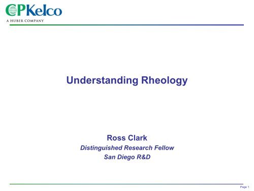
Understanding Rheology
Ross Clark
Distinguished Research Fellow
San Diego R&D
Page 1

CP Kelco makes carbohydrate based water soluble
polymers
– Fermentation
Xanthan
Gellan
– Plant derived
Pectin
Cellulose gum
Carrageenan
Thirty two years!
– Rheology
– Particle characterization (zeta potential, sizing)
– Microscopy
– Sensory science
– Unusual properties
Background
Page 2

Commonly used terms
Strain – Deformation or movement that occurs in a material.
Expressed as the amount of movement that occurs in a given
sample dimension this makes it dimensionless.
– Translation: How much did I move the sample?
Stress – Force applied to a sample expressed as force units per
unit area, commonly dynes/cm 2 or N/m 2 .
– Tranlation: How hard did I push, pull or twist the sample?
Viscosity –The ratio of shear stress/shear strain rate.
– Translation: How much resistance is there to flow?
Modulus – The ratio of stress / strain, expressed in force units
per unit area (since strain has no dimensions).
– Translation: How strong is the material?
Extensional viscosity – The resistance of a liquid to being pulled
Dynamic testing – The application of a sinusoidally varying
strain to a sample
Page 3

Types of deformation
Shear - A sliding deformation that occurs when there is
movement between layers in a sample, like fanning out a
deck of cards. May also be called torsion.
Compression - A pushing deformation that results from
pushing on two ends of a sample, like squeezing a grape.
Tension - A pulling deformation that occurs as you stretch
a sample, like pulling on a rubber band. May also be
called extension.
Page 4

Extension (Tension)
Bending
Simple Shear
Basic Deformations
Page 5

1 meter
separation
1 square meter area
1 Newton, force
1 meter/second, velocity
Shear
rate
Laminar Shear Flow
Shear
Stress
1 Newton
2
1 meter
Since viscosity is defined as shear stress/shear rate, the final units (in the SI system) for
viscosity are Newton•second / m 2 . This can also be given as a Pascal•second since a
Pascal is one Newton / m 2 .
In the more traditional physics units, the units of viscosity are dynes•seconds / cm 2 . This
is defined as 1 Poise
1 mPa•s (milliPascal•second) is equivalent to 1 cP (centiPoise).
1meter
/ second
1meter
Density is sometimes included for gravity driven capillary instruments. This unit is a
centiStoke.
1
second
Page 6

More terms…
Dynamic Mechanical Analysis – Typically, a solid material
is “pushed” in bending, tugging, or sliding in a repetitive
manner.
Common symbols used:
Type of deformation: Modulus values Strain Stress
Shear G, G’, G” G*
Compression /tension E, E’, E”, E*
Tan delta – The tangent of the phase angle, delta.
Obtained as the ratio of G’ and G” or E’ and E”
– Still used but actual phase angle ( ) seems more logical
Page 7

1. 2
- 1 . 2
Viscoelastic Response of a Perfectly Elastic Sample
0
Strain
Stress
Viscoelastic Response of a Perfectly Viscous Sample
1. 2
- 1 . 2
1. 2
- 1 . 2
0
0
Strain
Stress
Viscoelastic Response of a Xanthan Gum Sample
Strain
Stress
10 0
10 0
10 0
Viscoelasticity measurement
Elastic materials, like a steel spring, will always
have stress and strain when tested in dynamic
test. This is because the material transfers the
applied stress with no storage of the energy.
Viscous materials, like water or thin oils, will
always have stress and strain shifted 90° from
each other. This is because the most
resistance to movement occurs when the rate
of the movement is the greatest.
Most of the world is viscoelastic in nature and
so shares characteristics of elastic and viscous
materials. The phase shift ( ) will always be
between 0° and 90°.
Page 8

G” (viscous)
1 . 2
- 1 . 2
Viscoelastic Response of a Perfectly Elastic Sample
0
Strain
Stress
100
Where do G’ and G” come from?
Viscoelastic Response of a Perfectly Viscous Sample
1 . 2
- 1 . 2
0
Strain
Stress
100
1 . 2
- 1 . 2
0
Viscoelastic Response of a Xanthan Gum Sample
Convert to phase angle ( ) and magnitude
and then from polar to rectangular coordinates
G” (viscous)
G’ (elastic) G’ (elastic) G’ (elastic)
G” (viscous)
Strain
Stress
100
Page 9

What is the use of viscoelasticity?
As crosslinks form in a material, it shows more and more
elasticity.
As molecular weight increases, most systems become
more entangled, this results in more elasticity, especially
at high deformation rates.
Samples with a high degree of viscous response tend to
not stabilize and suspend as well.
Processing of samples that are too elastic can often be
difficult.
Page 10

Still more terms for steady shear
Rate dependent effects (how fast you shear)
– A sample that decreases in viscosity as rate increases is
pseudoplastic
Alignment of chains due to flow field decreases resistance
– Unusual samples can increase in viscosity as the rate goes up,
these are dilatent
Almost always are highly loaded suspensions with many particles that
lock together as the rate increase; can’t get out of the way
Time dependent effects (how long you shear)
– When viscosity goes down this is thixotropy; may or may not be
reversible after shear stops
If the network is robust, it is reversible
– Increasing viscosity is very rare, it is called rheopectic flow. You
may never see it!
Did you see shear thinning? No!
Page 11

Viscosity
Suspension
Stabilization
Commonly encountered shear rates
Sag and Leveling
Pouring
Mouthfeel
Dispensing
Pumping
Coating
Spraying
10
Shear Rate
-6 10-5 10-4 10-3 10-2 10-1 1 10 10 +2 10 +3 10 +4 10 +5 10 +6
Page 12

Couette Rheometers, Design
Couette, coaxial cylinder or cup and bob
• This type of “geometry” is
commonly used for materials that
contain suspended solids
• Providing the gap between the cup
and bob is small, the exact shear
rate can be determined
• Easy to control evaporation with an
oil layer on top
• Higher shear rates result in
unstable flow due to centrifugal
force
Page 13

Couette Calculations
Measured parameters: speed of rotation (rpm), torque (T),
bob radius (R b), bob height (H b) and cup radius (R c)
.
=
= 2 *
T
2 * * R b 2 * Hb
2 * * rpm
60
* Newtonian flow assumed, corrections will need to be made
for non-Newtonian fluids
*
R c 2
R c 2 - Rb 2
Page 14

Initial, t=0
The problem with Couette flow
Newtonian
Pseudoplastic
Cup Wall Bob Wall Cup Wall Bob Wall Cup Wall Bob Wall
Page 15

Couette, non–Newtonian Corrections
For all cases except where the gap between the cup & bob is very small, that is Rc/Rb > 0.95, we must
correct for the flow field in the gap. When a more pseudoplastic fluid is tested, the shear rate in the gap
tends to be the highest near the rotating member (the bob in the case of the Brookfield). This is because the
shear stress is at a maximum at this point and the fluid tends to flow faster under high shear stress values.
In any event, we need to correct for this flow profile in the gap. This is most commonly done by assuming
that the material will obey the power law, that is = K• n .
Below, a step by step procedure is listed for correction of the shear rate for non-Newtonian fluids in Couette
viscometers:
.
Step #1, calculate the shear stress, on the bob using the equation for Newtonian fluids.
Step #2, calculate the value of for each of the speeds used.
Step #3, make a log–log plot of and . Calculate the value of n (slope) and b (intercept).
Step #4, determine the correction factor, as: =
1+ [ln (s)/ n]
where s =
ln (s)
Step #5, determine the “K” value as K=b
. .
Step #6, determine the shear rate, as = •
Step #7, determine the viscosity, as
.
= /
n
R c 2
R b 2
Page 16

Couette Errors
In the table given below, the shear rate and errors associated with the Newtonian calculation of shear rate
for two different theoretical pseudoplastic fluids are given. In each case the speed of the viscometer is the
same (0.3 rpm) and the Rb/Rc calculation is given for the three different viscometer gaps.
It can be seen that the errors become very large for pseudoplastic fluids in wide gap instruments. This is
one reason to avoid the use of small spindles in the Brookfield small sample adapter or any other
viscometer.
Newtonian Pseudoplastic Error Pseudoplastic Error
Couette Gap n=1 n=0.658 (%) n=.261 (%)
Narrow 0.967 0.974 0.99 1.64% 1.063 9.14%
Moderate 0.869 0.255 0.271 6.27% 0.344 34.90%
Wide 0.672 0.11 0.127 15.45% 0.199 80.91%
An example of some of the dimensions for various Brookfield attachments is given in the table below. As you
can see, the error associated with even the “best” conditions (#18 bob with the small sample adapter or the
UL) is still significant, especially when the degree of pseudoplasticity of most of our fluids is taken into
account.
Bob Radius Cup Radius
(mm) (mm) Rb/Rc
Small Sample Adapter, #18 bob 8.7175 9.5175 0.916
Small Sample Adapter, #27 bob 5.8600 9.5175 0.616
UL Adapter 12.5475 13.8000 0.909
Page 17

Shear rate, (s -1 )
100
10
1
0.1
Brookfield LV with SSA #27 spindle
Kreiger-Elrod corrections applied
Nearly
2x higher
for xanthan!
Effect of Couette corrections
0.25% Keltrol
Glycerin / Water
1 10 100
Spindle speed (rpm)
Page 18

Cone and plate
Cone/Plate Rheometers, Design
• This type of “geometry” is
commonly used for clear fluids
without solids
• If the angle of the cone is less than
about 3°, there will be a uniform
shear rate in the gap
• Mind the gap! Particles can interfere
since a common gap is 50 microns
• A variation of this is the parallel
plate; a compromise in accuracy for
ease of use
Page 19

Cone/Plate Calculations
Measured parameters: speed of rotation (rpm), torque (T),
cone angle ( ) and cone radius (R c)
.
=
= 2 *
T
2 / 3 * * R c 3
2 * * rpm / 60
sine ( )
* Calculations are valid for Newtonian and non-Newtonian
materials
Page 20

Side or edge view
10 mm
Top View
1.5°
10 mm
20 mm
0.262 mm
20 mm
Cone & Plate Calculations
0.524 mm
Torque .
2/3 • • r3 If we assume a speed of 12 rpm or 1.26 rad/s:
Linear velocity @ 10 mm = 12.6 mm/sec
Linear velocity @ 20 mm = 25.2 mm/sec.
The shear strain rate is given by the velocity / separation:
Shear strain rate @ 10 mm = 48.1 s -1
Shear strain rate @ 20 mm = 48.1 s -1 .
In this example, we have
a cone with angle, and
a radius, r. Providing
that the cone angle is

Capillary or pipe flow
Capillary Rheometers, Design
• This type of “geometry” can be used
with either clear fluids or ones with
solids
• The device can be driven by a
constant pressure or a constant
volumetric flow
• Gravity driven glass instruments are
traditional for polymer Mw
• Excellent oscillatory instrument is
the Vilastic www.vilastic.com.
Superb accuracy for low viscosity
Page 22

Capillary Calculations
Measured parameters: capillary radius (Rc), capillary length
(Lc), volumetric flow rate (Q) and pressure drop ( p)
=
= 2 *
p * R c
2 * L c
4 * Q
* R c 3
* Newtonian flow assumed, corrections will need to be made
for non-Newtonian fluids
.
Page 23

Steady shear rheological models
Used to “reduce” the data to a standard equation.
May provide insight into molecular processes.
– Yield stress
– Association or crosslink half life
Are useful to engineers needing data to plug into standard
formulas (pumping, pressure drop, pipe size).
Page 24

Viscosity
Equation: = K *
10 3
10 2
10 -1
10 0
.
Newtonian
10 1
Rate
10 2
10 6
10 5
10 4
10 3
10 2
10 1
10 3
Shear stress
For this graph:
K = 150
Newtonian
Newtonian fluids are
rare. Low molecular
weight oils and some
small water soluble
polymer molecules.
Page 25

Viscosity
Equation: = o + (K *
10 3
10 2
10 -1
10 0
Bingham
10 1
Rate
.
10 2
10 6
10 5
10 4
10 3
10 2
10 1
10 3
Shear stress
Bingham Plastic
For this graph:
K = 120
o = 20
This modification of the
Newtonian model allows
for a yield stress. This
is a force that must be
exceeded before flow
can begin.
A frequently used oilfield
model (“YP” and
“PV”).
Page 26

Viscosity
Equation: = o + K *
10 3
10 2
10 1
10 -1
10 0
Casson model
10 1
Rate
10 2
.
10 5
10 4
10 3
10 2
10 1
10 3
Shear stress
For this graph:
K = 40
o = 20
Casson
This is a variation of the
Bingham model. It is
frequently used to
extrapolate to a yield
stress from low shear
rate data. Has been
successfully used with
chocolate.
Page 27

Viscosity
Equation: = K * n
.
10 3
10 2
10 1
10 0
10 -1
10 0
Power Law
10 1
Rate
10 2
10 4
10 3
10 2
10 1
10 3
Shear stress
Power Law
For this graph:
K = 150
n = 0.5
The power law model
is the most frequently
used equation. It fits
a wide range of water
soluble polymers to a
more or less
acceptable degree.
Xanthan gum is a
“classic” power law
fluid
Page 28

Viscosity
Equation: = o + K * ( n
.
10 3
10 2
10 1
10 0
10 -1
Ellis or power law + yield stress
10 0
10 1
Rate
10 2
Ellis (Power Law with Yield Stress)
10 4
10 3
10 2
10 1
10 3
Shear stress
For this graph:
K = 120
n = 0.5
o = 25
This modification of
the power law model
allows for a yield
stress like the
Bingham. It is difficult
to fit; 2 known
parameters, 3
unknowns.
Page 29

Viscosity
Equation: = +
10 3
10 2
10 1
10 0
10 -1
10 -2
10 -3
10 -7
10 -5
10 -3
Cross model
10 -1
Rate
1+ K * ( n
o –
.
10 1
10 3
10 5
10 4
10 3
10 2
10 1
10 0
10 -1
10 -2
10 -3
10 -4
Shear stress
Cross Model
For this graph:
= 0.002
o = 500
K = 50
n = 0.8
This model fits
viscosity data rather
than shear stress
data. It allows for
upper and lower
Newtonian viscosity
values. With 4
parameters, it
requires non–linear
methods.
Page 30

1% Xanthan in
0.05 M NaCl
50 mm parallel
plate, 0.5 mm
gap
23ªC
10 rad/s
50% strain
ARES instrument
G" ( )
[dyn/cm 2 ]
G' ( )
[dyn/cm 2 ]
10 3
10 2
10 1
0.0
1% xanthan in 0_05M NaCl ARES time sweep
50.0 100.0 150.0 200.0 250.0 300.0
time [s]
Time sweep test
350.0
Page 31

What is learned from a time sweep?
This is an essential first test to do on a material that is
unknown.
Tells you how long to wait to allow the sample to recovery
after loading.
Tells you how long you may need to wait between linked
tests.
Provides insight into recovery processes
Used with initial controlled shear to monitor recovery after
a process such a filling.
Page 32

1% Xanthan in
0.05 M NaCl
50 mm parallel
plate, 0.5 mm
gap
23ªC
10 rad/s
1 to 1000% strain
ARES instrument
G" ( )
[dyn/cm 2 ]
G' ( )
[dyn/cm 2 ]
10 3
10 2
10 1
10 0
10 0 10 1
1% xanthan in 0_05M NaCl ARES strain sweep
Line ar vis coelastic region
Strain [%]
10 2
Strain sweep test
10 3
Page 33

What is learned from the strain sweep?
How does applied strain effect the sample.
– Where does the structure begin to breakdown
– How quickly does it breakdown
Does the material have a linear viscoelastic region.
– Most do, that is where you normally do all further tests.
– How wide is this range?
Page 34

1% Xanthan in
0.05 M NaCl
50 mm parallel
plate, 0.5 mm
gap
23ªC
0.01 to 100 rad/s
50% strain
ARES instrument
G" ( )
[dyn/cm 2 ]
G' ( )
[dyn/cm 2 ]
10 3
10 2
10 1
10 -2 10 -1
1% xanthan in 0_05M NaCl ARES freq sweep
10 0
Freq [rad/s]
Frequency sweep test
10 1
10 2
Page 35

What is learned from a freq. sweep?
Tells us how time effects the sample.
– Materials usually become stronger (modulus increases) as the
rate increases or the measurement time decreases (rate = 1/time).
– If you can look at a material over a wide enough time range, most
things are the same.
– Cross over points for E’ and E” are commonly used as an
indication of the sample’s relaxation time (elastic and viscous
values are equal).
Page 36

1% bacterial
cellulose in tap
water
50 mm parallel
plate, 0.5 mm
gap
23ªC
Stress ramp from 0
to 100 dynes/cm 2
over a 120
second period
SR-2000
instrument
(t) ( )
[%]
1000.0
900.0
800.0
700.0
600.0
500.0
400.0
300.0
200.0
100.0
0.0
0.0
0.216% Primacel (0.36% total) in STW control
Yield stress:(2 0.59 dynes/cm 2 @ 139.57% strain)
5.0 10.0 15.0 20.0 25.0
(t) [dyn/cm 2 ]
Stress ramp test
30.0
Page 37

Best way to find a yield stress (catsup).
Why do a stress ramp test?
– By continually increasing the applied stress from zero to some
value that will get the material to flow, we can look for a break in
the curve.
– This break indicates when the material structure was substantially
broken.
Both the yield stress and yield strain are important.
Yield strain should be a little larger than the LVR limit.
Page 38

0.5% gellan gum
in 4 mM CaCl 2
50 mm parallel
plate, 0.5 mm
gap
23ªC
Dynamic test at
10 rad/s and 5%
strain
ARES instrument
with Peltier
heating / cooling
G' ( )
[dyn/cm 2 ]
10 3
10 2
10 1
4.0
55.0
Temperature sweep test
Figure 1. Effect of APV Gaulin Ho mogenizatio n on Gellan Gum Set Temperature
S et tem peratu re defined as G ' value
of 10 dynes/cm 2
C o ntrol T s ~ 97C
T re atm ent #1 T s 82C
T re atm ent #2 T s 74C
65.0 75.0 85.0
< ------ C ooling test run from high tem p to low < -------
Temp [°C]
95.0
Page 39

Commonly used to find T g in a material
Why do a temperature sweep test?
– Point at which the structure changes due to temperature
Used to find melting temperatures of samples.
– Materials like gelatin can change from a liquid to a solid
Find the amount of thinning that occurs with heating to
predict performance and design process equipment
Page 40

1% Xanthan in
0.05 M NaCl
50 mm parallel
plate, 0.5 mm
gap
23ªC
50 dynes / cm 2
stress
Strain(t) ( )
[%]
10 3
10 2
10 1
0.0
1% xanthan in 0_05M N aC l creep test
100.0 200.0 300.0 400.0 500.0 600.0 700.0 800.0
time [s]
Creep test
10 2
10 1
900.0
stress(t) ( )
[dyn/cm 2 ]
Page 41

What is learned from a creep test?
When a material is subjected to a constant stress (force) it
will flow easily if it has the characteristics of a liquid and
less if it is solid-like.
Can be used to fit data to spring-dashpot models.
Materials with a high amount of creep may be too fluid-like
(elastomers).
Some materials that are very elastic may not store energy
or dampen properly.
Page 42

E 2
E 1
Spring-represents a
perfectly elastic element
Spring and dashpot models
Used to provide a physical model of a material’s properties
strain
E 2+ - Relaxation time
time
Dashpot-represents a
perfectly viscous element
This represents an idealized creep curve with the data
fitting a single relaxation or retardation time. E 1
represents the initial elastic deformation, 1 represents
the creep flow or steady state viscosity and the E 2 + 2
combination provides a retarded flow that can be used to
determine a characteristic time of a material.
E 1
Page 43

1% Xanthan in
0.05 M NaCl
50 mm parallel
plate, 0.5 mm
gap
23ªC
50% strain
ARES instrument
S tra in (t) ( )
[% ]
10 2
10 1
10 0
1% xanthan in 0_05M NaC l AR ES s tres s relaxation tes t #3
Relaxation test
0 .0 5 0 .0 1 0 0 .0 1 5 0 .0 2 0 0 .0 2 5 0 .0
tim e [s ]
10 3
10 2
10 1
s tre s s (t) ( )
[d yn /cm 2 ]
W e d n e s d a y , S e p t e m b e r 0 6 , 2 0 0 0 R o s s C l a r
Page 44

stress(t) ( )
[Pa]
8.0
7.0
6.0
5.0
4.0
3.0
2.0
1.0
Startup (stress overshoot) test
0.0
0.0 100.0 200.0 300.0 400.0 500.0 600.0 700.0 800.0 900.0 1000.0
Strain [%]
Page 45

What is learned from a stress overshoot?
How does the sample behave as the structure is broken
down by a large strain
Comparable to a dynamic strain sweep
– The overshoot test is done in steady shear
– Applies more strain than strain sweep
– Strain is not oscillatory but steady
This mimics many filling and dispensing operations
Page 46

1% Xanthan in
0.05 M NaCl
50 mm parallel
plate, 0.5 mm
gap
23ªC
Frequency sweep
data collected
with auto stress
adjust. Strain
controlled from
20 to 50%
Creep data
collected at 50
dynes / cm 2 stress
SR-2000
instrument
G" ( )
[dyn/cm 2 ]
G' ( )
[dyn/cm 2 ]
10 3
10 2
10 1
10 -3 10 -2
Creep frequency transform
G', G" from 1% xanthan in 0_05M N aC l creep test
These data are from a transform ation of
the creep cu rve data.
10 -1
These data are from a frequency sw eep curve
Freq [rad/s]
10 0
10 1
10 2
Page 47

Why use a creep freq. transform?
Creep tests provide data at longer times.
Two tests (creep and frequency) + transformation can give
more data in less time that a single longer frequency test.
Use an applied stress that yields a creep strain roughly the
same as what was applied in the frequency sweep.
Use in reverse to predict creep from frequency sweep
data. Useful in your instrument is not controlled stress.
Page 48

1% Xanthan in
0.05 M NaCl
50 mm parallel
plate, 0.5 mm
gap
23ªC
Frequency sweep
data collected
with auto stress
adjust. Strain
controlled from
20 to 50%
Creep data
collected at 50
dynes / cm 2 stress
SR-2000
instrument
G" ( )
[dyn/cm 2 ]
G' ( )
[dyn/cm 2 ]
10 3
10 2
10 1
-3 10-2
10
Relaxation frequency transform
Solid lines from relaxation data Dashed lines from frequency sweep
10 -1
10 0
Freq [rad/s]
10 1
10 2
10 3
Page 49

Why use a relaxation freq transform?
Sometimes relaxation tests can collect data a shorter
times that other tests.
Extending the data to shorter times aids understanding.
This is a sort of “impact” test and can simulate some short
time processes.
Can serve as a confirmation of the data collected with
another type of test.
Use in reverse to obtain relaxation data from frequency
sweeps.
Page 50

Time Temperature Superposition
Characteristics of viscoelastic materials vary with both
time and temperature.
We can trade temperature for time and get more
information quickly
But…. Only if our material does not change state over the
chosen temperature range
Page 51

0.5% gellan gum
in 4 mM CaCl 2
25 mm parallel
plate, 0.5 mm
gap
-35 to +55ªC
Frequency sweep
data collected at
10% strain
ARES instrument
G" ( )
[dyn/cm 2 ]
G' ( )
[dyn/cm 2 ]
10 6
10 5
10 4
10 3
10 2
10 1
10 -1 10 0
[Pg13]:TTS Session--TTS Overlay Curve
10 1
Freq [rad/s]
10 2
TTS data
10 3
Page 52

Data shifted with
two dimensional
residual
minimization.
Cubic spline
interploation
G" ( )
[dyn/cm 2 ]
G' ( )
[dyn/cm 2 ]
10 7
10 6
10 5
10 4
10 3
10 2
10 -6 10 -5
[Pg18]:TTS Session--TTS Overlay Curve
10 -4
10 -3
10 -2
Freq [rad/s]
For more information concerning minimization methods developed by Brent and Powell, see W. H.
Press, et. al., Numerical Recipes in C, Cambridge University Press, 1992, ISBN 0 521 43108
TTS data after shifting
10 -1
10 0
10 1
10 2
Page 53

G" ( )
[dyn/cm 2 ]
G' ( )
[dyn/cm 2 ]
10 7
10 6
10 5
10 4
10 3
10 2
10 -6 10 -5
10 -4
10 -3
10 -2
Freq [rad/s]
10 -1
TTS master curve
10 0
10 1
10 2
90.0
80.0
70.0
60.0
50.0
40.0
30.0
20.0
10.0
0.0
PhaseAngle ( )
[°]
Page 54

Practical tips 1
Know your instrument
– Torque limits
Most manufacturers stretch the truth; confirm with standards!
– Rotational speed limits
Computerized instrument isolate the user; you need to know if you are
asking the impossible
– Frequency limits
Very low frequencies might not be accurate
High frequencies might have “roll off” in strain or inertial problems
– Strain limits
In a digital world there is a limit to the bits of resolution
No substitute for being able to see the actual waveforms
– Temperature accuracy
Don’t assume it is correct!
Does the temperature controller over or undershoot
Controlled stress instruments are a problem
– Samples fundamentally react to strain
Page 55

Practical tips 2
Pick the best test geometry
– Cone and plate is ideal
Small volume
Uniform shear rate
Can’t be used with varying temperatures
Can’t be used if solid particles > 25% of the gap are present
– Common gap is 50 microns!
– Parallel plate a workable compromise
Not a uniform shear strain or rate
Relatively insensitive to temperature changes
Handles solid particles better
– Common gap is 1 mm
Reduce the gap to 50-100 microns to achieve a higher shear rate
– Couette is good for larger samples
Usually need 5-20 ml samples
Easier to control evaporation
Needs corrections in most cases.
Poor choice for high shear (Taylor instabilities)
Page 56

Sample loading sensitivity
– Select the best way to load the sample
Cast or form a gel in place
Cut a gel and put between parallel plates
Spoon or pipette
– Use time sweeps to determine the effects of loading
How long to wait before you begin testing
– Determine if evaporation control is important
Either recovery time or temperature are considered
Strain limits (stay in the Linear Viscoelastic Region)
– In most cases you have to work here
Practical tips 3
Consider the LVR when picking frequency sweep parameters
Can your instrument control strain?
Does it back up and start over if the strain limit is exceeded?
Consider the LVR strain when picking a creep stress
Page 57

What are you really interested in?
Practical tips 4
– Don’t measure samples blindly; consider what is important
– This is not reading tea leaves! Be selective with testing
For a uniform type of sample with small variations:
– No time or strain sweeps needed
– Mw and crosslinking can be measured with a frequency sweep
– Monitor modulus as a function of time?
– Is melt important?
If samples vary widely:
– LVR strain is likely to vary; an important characteristic
– Network rearrangement can be measured with creep
– Setting or melting might be revealing
Page 58

Most overlooked tests
Creep (constant stress)
– How networks rearrange
– Transformation to convert to frequency sweep
Step shear rate
– Low High Low for time dependency
– Never, ever, use a thixotropic loop test – Please!
Temperature ramps
– Even if TTS is not used, can still find about phase changes
– TTS cannot be used if there is a phase change!
Stress ramp
– Many materials have a functional yield stress
– Philosopical arguments aside, yield stress is practically present in
many materials
Oscillatory capillary test (Vilastic)
– Developed for biological fluids with weak structures
Page 59

Flow curve (viscosity versus shear rate)
– Are steady shear tests even appropriate
– Did thixotropy get covered up?
– Increase or decreasing speed?
– Steady increase (ramp) or stepwise (sweep)?
Thixotropic loop
– Ramp up and down
– Area in between supposed to be thixotropy
– Often is inertia in the instrument instead
Most overused tests
Page 60

In conclusion
Rheology is complex but understandable
– Experts often are not consulted (ask, we want to teach!)
– Expertise is more important than intuition about what test to use
Tremendous evolution in the last 15 years
– Historical literature can be a disadvantage; start fresh
A great deal of misinformation in the literature
– For example, lack of strain control in “stress controlled”
instruments
– Manufacturers are not good sources of information
Some exaggeration and distortion
Still more tests available:
– Solids testing
– Extensional properties of fluids
– Optical rheology
– Micro-rheology
Page 61