Spectral Characterisation of the Osterseen Lake District - EARSeL ...
Spectral Characterisation of the Osterseen Lake District - EARSeL ...
Spectral Characterisation of the Osterseen Lake District - EARSeL ...

Create successful ePaper yourself
Turn your PDF publications into a flip-book with our unique Google optimized e-Paper software.
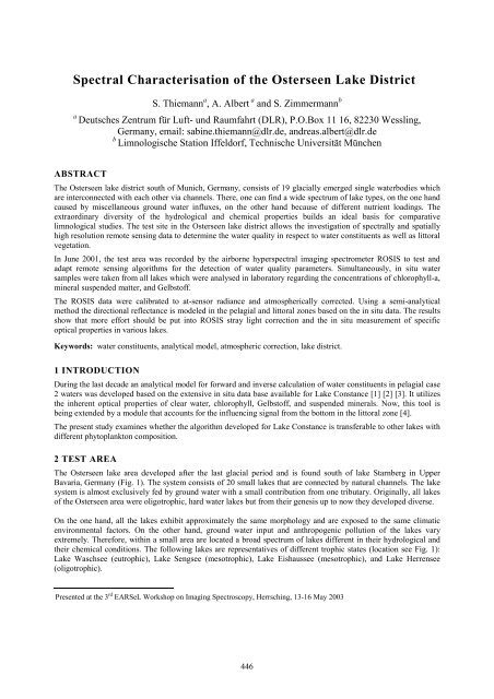
<strong>Spectral</strong> <strong>Characterisation</strong> <strong>of</strong> <strong>the</strong> <strong>Osterseen</strong> <strong>Lake</strong> <strong>District</strong> <br />
S. Thiemann a , A. Albert a and S. Zimmermann b<br />
a Deutsches Zentrum für Luft- und Raumfahrt (DLR), P.O.Box 11 16, 82230 Wessling,<br />
Germany, email: sabine.thiemann@dlr.de, andreas.albert@dlr.de<br />
b Limnologische Station Iffeldorf, Technische Universität München<br />
ABSTRACT<br />
The <strong>Osterseen</strong> lake district south <strong>of</strong> Munich, Germany, consists <strong>of</strong> 19 glacially emerged single waterbodies which<br />
are interconnected with each o<strong>the</strong>r via channels. There, one can find a wide spectrum <strong>of</strong> lake types, on <strong>the</strong> one hand<br />
caused by miscellaneous ground water influxes, on <strong>the</strong> o<strong>the</strong>r hand because <strong>of</strong> different nutrient loadings. The<br />
extraordinary diversity <strong>of</strong> <strong>the</strong> hydrological and chemical properties builds an ideal basis for comparative<br />
limnological studies. The test site in <strong>the</strong> <strong>Osterseen</strong> lake district allows <strong>the</strong> investigation <strong>of</strong> spectrally and spatially<br />
high resolution remote sensing data to determine <strong>the</strong> water quality in respect to water constituents as well as littoral<br />
vegetation.<br />
In June 2001, <strong>the</strong> test area was recorded by <strong>the</strong> airborne hyperspectral imaging spectrometer ROSIS to test and<br />
adapt remote sensing algorithms for <strong>the</strong> detection <strong>of</strong> water quality parameters. Simultaneously, in situ water<br />
samples were taken from all lakes which were analysed in laboratory regarding <strong>the</strong> concentrations <strong>of</strong> chlorophyll-a,<br />
mineral suspended matter, and Gelbst<strong>of</strong>f.<br />
The ROSIS data were calibrated to at-sensor radiance and atmospherically corrected. Using a semi-analytical<br />
method <strong>the</strong> directional reflectance is modeled in <strong>the</strong> pelagial and littoral zones based on <strong>the</strong> in situ data. The results<br />
show that more effort should be put into ROSIS stray light correction and <strong>the</strong> in situ measurement <strong>of</strong> specific<br />
optical properties in various lakes.<br />
Keywords: water constituents, analytical model, atmospheric correction, lake district.<br />
1 INTRODUCTION<br />
During <strong>the</strong> last decade an analytical model for forward and inverse calculation <strong>of</strong> water constituents in pelagial case<br />
2 waters was developed based on <strong>the</strong> extensive in situ data base available for <strong>Lake</strong> Constance [1] [2] [3]. It utilizes<br />
<strong>the</strong> inherent optical properties <strong>of</strong> clear water, chlorophyll, Gelbst<strong>of</strong>f, and suspended minerals. Now, this tool is<br />
being extended by a module that accounts for <strong>the</strong> influencing signal from <strong>the</strong> bottom in <strong>the</strong> littoral zone [4].<br />
The present study examines whe<strong>the</strong>r <strong>the</strong> algorithm developed for <strong>Lake</strong> Constance is transferable to o<strong>the</strong>r lakes with<br />
different phytoplankton composition.<br />
2 TEST AREA<br />
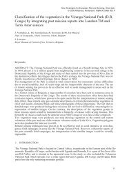
The <strong>Osterseen</strong> lake area developed after <strong>the</strong> last glacial period and is found south <strong>of</strong> lake Starnberg in Upper<br />
Bavaria, Germany (Fig. 1). The system consists <strong>of</strong> 20 small lakes that are connected by natural channels. The lake<br />
system is almost exclusively fed by ground water with a small contribution from one tributary. Originally, all lakes<br />
<strong>of</strong> <strong>the</strong> <strong>Osterseen</strong> area were oligotrophic, hard water lakes but from <strong>the</strong>ir genesis up to now <strong>the</strong>y developed diverse.<br />
On <strong>the</strong> one hand, all <strong>the</strong> lakes exhibit approximately <strong>the</strong> same morphology and are exposed to <strong>the</strong> same climatic<br />
environmental factors. On <strong>the</strong> o<strong>the</strong>r hand, ground water input and anthropogenic pollution <strong>of</strong> <strong>the</strong> lakes vary<br />
extremely. Therefore, within a small area are located a broad spectrum <strong>of</strong> lakes different in <strong>the</strong>ir hydrological and<br />
<strong>the</strong>ir chemical conditions. The following lakes are representatives <strong>of</strong> different trophic states (location see Fig. 1):<br />
<strong>Lake</strong> Waschsee (eutrophic), <strong>Lake</strong> Sengsee (mesotrophic), <strong>Lake</strong> Eishaussee (mesotrophic), and <strong>Lake</strong> Herrensee<br />
(oligotrophic).<br />
Presented at <strong>the</strong> 3 rd <strong>EARSeL</strong> Workshop on Imaging Spectroscopy, Herrsching, 13-16 May 2003<br />
446
3 DATA<br />
Hamburg<br />
Germany<br />
Munich<br />
Berlin<br />
Lustsee Grobensee<br />
N<br />
Westl.<br />
Breitenauersee<br />
Härtlings Sill<br />
Lintensee<br />
Stechsee<br />
Ameisensee<br />
Östl. Breitenauersee<br />
Ground Water<br />
Wellspring<br />
Großer Ostersee<br />
Eishaussee<br />
Brauhaussee<br />
Herrensee<br />
Fischkaltersee<br />
Forchensee<br />
Wolfelsee<br />
Sengsee<br />
Fohnsee<br />
Schiffhüttensee<br />
Waschsee<br />
Figure 1. Location <strong>of</strong> <strong>the</strong> test area "<strong>Osterseen</strong> <strong>Lake</strong> <strong>District</strong>" south <strong>of</strong> Munich, Germany.<br />
0 500 m<br />
3.1. Hyperspectral remote sensing data acquired by ROSIS sensor<br />
The Reflective Optics System Imaging Spectroradiometer (ROSIS) was developed since 1986 in cooperation<br />
between DLR, GKSS, and MBB (now Astrium) [5][6][7]. It is a push broom scanner with 512 spatial and 115<br />
spectral pixels recording in <strong>the</strong> wavelength range between 430 nm and 860 nm. The spectral sampling interval<br />
amounts 4 nm and <strong>the</strong> full width at half maximum is about 7.5 nm. With an instantaneous field <strong>of</strong> view <strong>of</strong> 0.59<br />
mrad <strong>the</strong> spatial resolution results in 2.8 x 2.8 m² at a flight altitude <strong>of</strong> 5,000 m.<br />
The data presented in this study were recorded on June 5 th , 2001 between 10:42 and 11:20 UTC in a nor<strong>the</strong>rly flight<br />
direction at an altitude <strong>of</strong> about 5,000 m. The data were radiometrically corrected based on laboratory<br />
measurements using a calibrated light source. The geometric correction <strong>of</strong> <strong>the</strong> distortions due to flight attitude (roll,<br />
pitch, and yaw angles) uses information from <strong>the</strong> airplane's inertial system, <strong>the</strong> flight velocity, <strong>the</strong> altitude above<br />
ground, and <strong>the</strong> focal length <strong>of</strong> <strong>the</strong> telescope [8]. The radiometrically and geometrically corrected composit <strong>of</strong> two<br />
flight lines is shown in Fig. 2.<br />
447
Figure 2. Subset from two ROSIS flight lines acquired on June 5 th , 2001 - true color band composit after<br />
radiometric calibration and geometric rectification. Points <strong>of</strong> in situ measurements and drawn spectra<br />
448
3.2. In situ data<br />
Simultaneously to <strong>the</strong> overflights, water samples were taken and Secchi depth was measured in each lake <strong>of</strong> <strong>the</strong><br />
<strong>Osterseen</strong> <strong>Lake</strong> <strong>District</strong> at 1m and 3 m water depth, and in cases <strong>of</strong> high Secchi depth also at 5 m. The samples<br />
were analysed in <strong>the</strong> laboratory for <strong>the</strong> optically relevant water constituents chlorophyll, suspended matter, and<br />
Gelbst<strong>of</strong>f. Chlorophyll analysis was conducted by photometric measurement <strong>of</strong> <strong>the</strong> transmission <strong>of</strong> <strong>the</strong> solution at<br />
665 nm and 750 nm after <strong>the</strong> samples were filtered through a 1 µm filter, extracted [9], and centrifugated.<br />
Suspended matter was measured as total, organic, and inorganic concentration. The water samples were filtered<br />
through a dried and weighed 1 µm glass fiber filter and dried for two hours at 105°C and <strong>the</strong>n for four hours at<br />
550°C with weighing after each step. The total suspended matter is <strong>the</strong> dry weight after <strong>the</strong> first step subtracted by<br />
<strong>the</strong> filter weight, <strong>the</strong> inorganic matter is <strong>the</strong> weight after <strong>the</strong> second step, and <strong>the</strong> organic matter is <strong>the</strong> loss between<br />
<strong>the</strong>se two weighings. For <strong>the</strong> determination <strong>of</strong> <strong>the</strong> Gelbst<strong>of</strong>f absorption, <strong>the</strong> water samples were sucked through a<br />
0.2 µm filter. The transmission was measured with a Perkin-Elmer Lambda-2 dual beam spectrophotometer in 10<br />
cm and 5 cm cuvettes. From <strong>the</strong>se two transmission spectra <strong>the</strong> Gelbst<strong>of</strong>f absorption was determined including <strong>the</strong><br />
pure water correction using <strong>the</strong> absorption spectrum from [10]. The in situ data are given in Tab. 1 including also<br />
<strong>the</strong> spectral slope to additionally characterize Gelbst<strong>of</strong>f spectrally.<br />
Table 1. In situ measurements <strong>of</strong> water constituents on June 5 th , 2001<br />
<strong>Lake</strong> Secchi Depth Chlorophyll-a Total suspended Gelbst<strong>of</strong>f [m<br />
[m]<br />
[µg/l] Matter [mg/l]<br />
-1 ] Gelbst<strong>of</strong>f<br />
<strong>Spectral</strong> Slope S<br />
Waschsee [1 m] 1.9 6.2 0.9 0.62 0.0150<br />
[3 m] 41.7 4.6 0.77 0.0138<br />
Schiffhüttensee [1 m] 1.5 16.7 3.4 0.65 0.0133<br />
[3 m] 22.4 4.9 0.53 0.0147<br />
Sengsee [1 m] 3.8 2.0 1.5 - -<br />
[3 m] 2.0 2.9 0.69 0.0142<br />
Fohnsee [1 m] 6.9 0.5 0.6 0.64 0.0134<br />
[3 m] 2.0 0.9 0.15 0.0114<br />
Westl. Eishaussee [1 m] 5.0 0.9 0.7 0.52 0.0148<br />
[3 m] 1.7 1.7 0.41 0.0132<br />
Östl. Eishaussee [1 m] 4.9 1.2 0.5 0.43 0.0137<br />
[3 m] 2.3 1.4 0.58 0.0148<br />
Gr. Ostersee - S [1 m] 1.9 1.8 2.3 - -<br />
[3 m] 1.8 3.2 0.32 0.0152<br />
Gr. Ostersee - N [1 m] 1.5 2.2 2.2 0.41 0.0117<br />
[3 m] 1.8 2.9 0.38 0.0125<br />
Westl. Breitenauersee [1 m] 3.5 1.2 1.9 0.36 0.0126<br />
[3 m] 1.2 1.9 0.56 0.0154<br />
Lustsee [1 m] 7.5 - 0.4 0.67 0.0143<br />
[3 m] 0.9 - 0.49 0.0139<br />
[5 m] 0.2 1.0 - -<br />
Stechsee [1 m] 4.5 0.7 4.1 0.57 0.0145<br />
[3 m] 0.6 3.7 1.08 0.0116<br />
449
4 METHODS<br />
4.1. Analytical modeling <strong>of</strong> remote sensing reflectance<br />
The output spectra after <strong>the</strong> atmospheric correction (see chapter 4.2) are given in units <strong>of</strong> reflectance above <strong>the</strong><br />
surface, R + = <br />
R rs + L. The first part represents <strong>the</strong> remote sensing reflectance <strong>of</strong> <strong>the</strong> water, and <strong>the</strong> second part <strong>the</strong><br />
reflectance <strong>of</strong> <strong>the</strong> water surface. The spectra measured by ROSIS are corrected for <strong>the</strong> surface effect by comparing<br />
<strong>the</strong> infrared wavelengths with simulated spectra using <strong>the</strong> in situ measurements. The factor <strong>of</strong> <strong>the</strong> reflected sky<br />
radiance L is obtained iterative.<br />
The underwater remote sensing reflectance is modeled according to [4] by a set <strong>of</strong> analytical equations including<br />
shallow water. The parameterizations were developed using simulations <strong>of</strong> <strong>the</strong> radiative transfer program<br />
Hydrolight (version 3.1), which is explained in detail by [12]. The remote sensing reflectance below <strong>the</strong> water<br />
surface is <strong>the</strong> sum <strong>of</strong> two parts: <strong>of</strong> <strong>the</strong> water body and <strong>of</strong> <strong>the</strong> bottom, Rrs,W and Rrs,B. These two parts can be<br />
expressed as follows:<br />
<br />
K <br />
<br />
<br />
<br />
u , W R K<br />
B<br />
u,<br />
B<br />
R<br />
<br />
<br />
<br />
rs Rrs,<br />
W Rrs,<br />
B f x 1<br />
A1<br />
exp <br />
<br />
<br />
<br />
<br />
<br />
<br />
<br />
<br />
Kd<br />
<br />
<br />
zB<br />
A2<br />
exp Kd<br />
zB<br />
cos<br />
v <br />
cos<br />
v <br />
with <strong>the</strong> f-factor <strong>of</strong> <strong>the</strong> remote sensing reflectance and <strong>the</strong> attenuation coefficients <strong>of</strong> <strong>the</strong> downwelling irradiance,<br />
<strong>the</strong> upwelling irradiance <strong>of</strong> <strong>the</strong> water body, and <strong>the</strong> upwelling irradiance reflected from <strong>the</strong> bottom – Kd, Ku,W, and<br />
Ku,B respectively:<br />
<br />
2 3 p <br />
5 p6<br />
f p <br />
<br />
1 1 p2x<br />
p3x<br />
p4x<br />
<br />
1<br />
<br />
1<br />
,<br />
cos<br />
s cos<br />
v <br />
a bb<br />
K d 0 , <br />
cos<br />
<br />
s<br />
<br />
<br />
1 , W<br />
2,<br />
W<br />
K <br />
u,<br />
W a bb<br />
1 x<br />
<br />
1<br />
, and <br />
cos<br />
<br />
s <br />
<br />
<br />
1 , B<br />
2,<br />
B<br />
K <br />
u,<br />
B a bb<br />
1 x<br />
<br />
1<br />
.<br />
cos<br />
s <br />
The parameter x is <strong>the</strong> ratio bb/(a+bb) with <strong>the</strong> total absorption a and <strong>the</strong> backscattering coefficient bb. The sun<br />
position is given by <strong>the</strong> solar zenith angle below <strong>the</strong> water surface s, <strong>the</strong> viewing position by v. The<br />
parameterization regards <strong>the</strong> influence <strong>of</strong> <strong>the</strong> bottom reflectance RB at <strong>the</strong> bottom depth zB. The absorption a and <strong>the</strong><br />
backscattering coefficient bb are calculated using a bio-optical model developed by [13] and [14] for <strong>Lake</strong><br />
Constance. The total absorption is <strong>the</strong> sum <strong>of</strong> <strong>the</strong> absorption <strong>of</strong> pure water, Gelbst<strong>of</strong>f, and phytoplankton. The<br />
backscattering coefficient is determined by <strong>the</strong> backscattering <strong>of</strong> <strong>the</strong> pure water [10] and <strong>of</strong> suspended matter. The<br />
coefficients Ai, pj, and k were obtained by a multiple regression analysis <strong>of</strong> all Hydrolight simulations using a<br />
Marquardt-Levenberg fit. The values <strong>of</strong> <strong>the</strong> coefficients are listed in Tab. 2. The analytical equations <strong>of</strong> <strong>the</strong> remote<br />
sensing reflectance are used for forward modeling <strong>of</strong> spectra <strong>of</strong> <strong>the</strong> lakes and for inversion <strong>of</strong> airborne data <strong>of</strong><br />
ROSIS as well. The inversion technique uses <strong>the</strong> Simplex algorithm after [15].<br />
Table 2: Coefficients for <strong>the</strong> model <strong>of</strong> <strong>the</strong> remote sensing reflectance.<br />
A1 1.1576 p1 0.0512 sr -1<br />
A2 1.0389 sr<br />
0 1.0546<br />
-1<br />
p2 4.6659 1,W 3.5421<br />
p3 -7.8387 2,W -0.2786<br />
p4 5.4571 1,B 2.2658<br />
p5 0.1098 2,B 0.0577<br />
p6 0.4021<br />
4.2. Atmospheric correction <strong>of</strong> <strong>the</strong> ROSIS data<br />
The ROSIS data were atmospherically corrected using <strong>the</strong> ATCOR4 program based on MODTRAN calculations<br />
[16][17]. It accounts for <strong>the</strong> irradiation characteristics <strong>of</strong> <strong>the</strong> sun, for molecule and aerosol scattering in <strong>the</strong><br />
atmosphere, for <strong>the</strong> scan angle effect <strong>of</strong> additional atmospheric path with distance to nadir view, and for <strong>the</strong><br />
adjacency effect from <strong>the</strong> nearby environment. The necessary input parameters including altitude, specific<br />
insolation, and atmospheric variables are shown in Tab. 3. They were considered constant for <strong>the</strong> time slot <strong>of</strong> data<br />
take.<br />
450
Table 3. Input parameter for atmospheric correction <strong>of</strong> <strong>the</strong> ROSIS flight lines<br />
flight altitude [km] 5.65<br />
ground altitude ab. sea level [km] 0.59<br />
sun zenith angle [°] 25.2<br />
sun azimuth angle [°] 181.1<br />
flight heading [90°east] 351<br />
day <strong>of</strong> <strong>the</strong> year 155<br />
water vapor content [g cm - ²] 2.0<br />
aerosole type rural<br />
visibility [km] 25.0<br />
adjacency box [Pixel] 30<br />
By inflight calibration experiments one can generally check <strong>the</strong> validity <strong>of</strong> <strong>the</strong> laboratory calibration. The<br />
radiometric performance <strong>of</strong> an airborne sensor may differ from <strong>the</strong> one in laboratory due to <strong>the</strong> aircraft environment<br />
and <strong>the</strong> longer distance between <strong>the</strong> sensor and <strong>the</strong> target influencing stray light effects in <strong>the</strong> blue wavelength<br />
range. Therefore, for <strong>the</strong> present study different calibration coefficients have been generated and tested using <strong>the</strong><br />
inflight calibration module in ATCOR 4 (see Fig. 3). It appeared that <strong>the</strong> resulting atmospherically corrected<br />
reflectance spectra are very sensitive to variations with <strong>the</strong>se coefficients. The best results compared to modeled<br />
spectra <strong>of</strong> selected lakes were achieved by applying <strong>the</strong> coefficients partly derived from inflight calibration with a<br />
shallow water area in <strong>Lake</strong> Ostersee with logarithmic interpolation between 478 nm and 730 nm (see Fig. 3 h).<br />
Figure 4 shows an intercomparison between modeled spectra (Fig. 4) for four selected lakes (including one shallow<br />
water spectrum modeled for 1 m water depth over sandy sediment) and atmospherically corrected ROSIS spectra <strong>of</strong><br />
<strong>the</strong> same location using 3 x 3 pixel mean values. The shallow water spectrum (No. 13) can be reproduced similarly<br />
using <strong>the</strong> forward model. The deep water spectra are in <strong>the</strong> same order <strong>of</strong> magnitude, however <strong>the</strong> reflectance<br />
between 450 nm and 550 nm is sometimes higher in <strong>the</strong> ROSIS spectra.<br />
Arbitrary units<br />
0.004<br />
0.0035<br />
0.003<br />
0.0025<br />
0.002<br />
0.0015<br />
0.001<br />
0.0005<br />
0<br />
400 450 500 550 600 650 700 750 800 850<br />
Wavelength [nm]<br />
Figure 3. Calibration coefficients tested for atmospheric correction a) standard coefficients, b) generated from<br />
inflight calibration at a different test site "Nantes", c) generated from inflight calibration with modeled spectrum<br />
<strong>Lake</strong> Ostersee shallow water (Fig. 2, No. 13), d) generated from inflight calibration with modeled spectrum <strong>Lake</strong><br />
Fohnsee (Fig. 2, No. 7), e) generated from inflight calibration with modeled spectrum <strong>Lake</strong> Sengsee (Fig. 2, No.<br />
10), f) joined coefficients from 3c below 450 nm and from 3b above 450 nm, g) mean from coefficients 3b and 3c,<br />
and h) coefficients from 3c with logarithmic interpolation between 478 nm and 730 nm.<br />
5 DATA ANALYSIS AND INTERPRETATION<br />
For all lakes mentioned in Tab. 1, <strong>the</strong> reflectance was modeled based on <strong>the</strong> concentration <strong>of</strong> water constituents as<br />
measured in situ (Fig. 5a). In Fig. 4, <strong>the</strong> corresponding ROSIS spectra were extracted with <strong>the</strong> mean value <strong>of</strong> a 3 x 3<br />
pixel matrix. For some lakes like <strong>Lake</strong> Ostersee (sou<strong>the</strong>rn basin) or <strong>Lake</strong> Breitenauer See (western basin), <strong>the</strong><br />
451<br />
a<br />
b<br />
c<br />
d<br />
e<br />
f<br />
g<br />
h
ROSIS spectra match quite well with <strong>the</strong> modeled spectra (see Fig. 4 a-c). However, several reasons exist why <strong>the</strong><br />
o<strong>the</strong>r ROSIS spectra (see Fig. 4 d) do not match with <strong>the</strong> modeled ones:<br />
1. Radiometric calibration <strong>of</strong> <strong>the</strong> sensor has to be improved (stray light).<br />
2. Atmospheric correction should be more accurately (adjacency effect, aerosol type).<br />
3. Sunglint has to be accounted for more accurately.<br />
4. It should be investigated how <strong>the</strong> optical properties <strong>of</strong> water constituents (phytoplankton absorption,<br />
backscattering <strong>of</strong> suspended matter) vary from test site to test site.<br />
5. The model may be improved including e.g. fluorescence, surface effects.<br />
Reflectance [%]<br />
Reflectance [%]<br />
14<br />
12<br />
10<br />
8<br />
6<br />
4<br />
2<br />
0<br />
400 450 500 550 600 650 700 750 800 850<br />
Wavelength [nm]<br />
30<br />
25<br />
20<br />
15<br />
10<br />
5<br />
0<br />
400 450 500 550 600 650 700 750 800 850<br />
Wavelength [nm]<br />
a) 14<br />
b)<br />
Reflectance [%]<br />
0<br />
400 450 500 550 600 650 700 750 800 850<br />
Wavelength [nm]<br />
Figure 4. Modelled (blue and orange) spectra in comparison with ROSIS (green and red) spectra for <strong>the</strong> lakes a)<br />
Ostersee (sou<strong>the</strong>rn basin) (see Fig. 2 No. 1), b) Breitenauersee (western basin) (see Fig. 2 No. 3), c) shallow water<br />
with 1 m bottom depth in sou<strong>the</strong>rn Ostersee (see Fig. 2 No. 13), and d) Sengsee (see Fig. 2 No. 10)<br />
6 CONCLUSION<br />
The ROSIS data from <strong>Osterseen</strong> lake district with various concentrations <strong>of</strong> water constituents show great potential<br />
for algorithm testing – especially regarding shallow water areas. The above mentioned influencing factors will be<br />
examined more closely in fur<strong>the</strong>r evaluations. In future, special focus will be put on stray light correction <strong>of</strong> <strong>the</strong><br />
ROSIS sensor and on optical in situ measurements to obtain a more accurate calibration <strong>of</strong> <strong>the</strong> sensor. More effort<br />
will be put on <strong>the</strong>. Also a data base <strong>of</strong> various specific optical properties will to be set up.<br />
A processing chain to derive water constituents from any hyperspectral sensor, modular inversion program for<br />
water (MIP-w), is under development in our group [14]. The advantage <strong>of</strong> MIP-w is to produce distribution maps<br />
from hyperspectral remote sensing data.<br />
12<br />
10<br />
8<br />
6<br />
4<br />
2<br />
c) 14<br />
d)<br />
Reflectance [%]<br />
452<br />
12<br />
10<br />
8<br />
6<br />
4<br />
2<br />
0<br />
400 450 500 550 600 650 700 750 800 850<br />
Wavelength [nm]
ACKNOWLEDGMENTS<br />
Part <strong>of</strong> <strong>the</strong> work is done in <strong>the</strong> frame <strong>of</strong> <strong>the</strong> Special Collaborative Program 454 "<strong>Lake</strong> Constance Littoral" provided<br />
by fundings <strong>of</strong> <strong>the</strong> German Research Foundation DFG. The in situ data were analyzed for water consitutents by<br />
Biologiebüro Weyhmüller. Peter Gege supported us with his WASI program and <strong>the</strong> Gelbst<strong>of</strong>f analysis. We thank<br />
Rolf Richter for providing and introducing <strong>the</strong> ATCOR program. The Hydrolight code was provided by C.D.<br />
Mobley.<br />
[1] REFERENCES<br />
[1] GEGE, P., 1994: Gewässeranalyse mit passiver Fernerkundung: Ein Modell zur Interpretation optischer<br />
Spektralmessungen. DLR-Forschungsbericht 94-15, 171 p.<br />
[2] GEGE, P., 2001: The water colour simulator WASI: A s<strong>of</strong>tware tool for forward and inverse modeling <strong>of</strong> optical<br />
in-situ spectra. Proc. IGARSS, Sydney, Australia, 9-13 July 2001.<br />
[3] GEGE, P., 2003: WASI - A s<strong>of</strong>tware tool for water spectra. Backscatter, Winter 2003, pp. 22-24.<br />
[4] ALBERT, A., 2002: Dependency <strong>of</strong> <strong>the</strong> remote sensing signal in shallow waters on solar and viewing angle.<br />
Proceedings <strong>of</strong> <strong>the</strong> XVI Ocean Optics Conference, Santa Fe, USA, 18-22 Novemer 2002.<br />
[5] KUNKEL, B., BLECHINGER, F., VIEHMANN, D., VAN DER PIEPEN, H. & DOEFFER, R., 1991: ROSIS imaging<br />
spectrometer and its potential for ocean parameter measurements (airborne and spaceborne). International Journal<br />
<strong>of</strong> Remote Sensing 12:4, pp. 753-761.<br />
[6] VAN DER PIEPEN, H., 1995: Nutzung und Anwendung des abbildenden Spektrometers ROSIS. DLR-Nachrichten<br />
77, pp. 11-14.<br />
[7] GEGE, P., BERAN, D., MOOSHUBER, W. , SCHULZ, J. & VAN DER PIEPEN H., 1998: System Analysis and<br />
Performance <strong>of</strong> <strong>the</strong> New Version <strong>of</strong> <strong>the</strong> Imaging Spectrometer ROSIS. First <strong>EARSeL</strong> Workshop on Imaging<br />
Spectroscopy, Remote Sensing Laboratories, University <strong>of</strong> Zurich, Switzerland, 6-8th October 1998.<br />
[8] MÜLLER, RU., LEHNER, M., MÜLLER, RA., REINARTZ, P., SCHROEDER, M. & VOLLMER, B., 2002: A program<br />
for direct georeferencing <strong>of</strong> airborne and spaceborne line scanner images. Proceedings <strong>of</strong> ISPRS Commission I Mid-<br />
Term Symposium "Integrating Remote Sensing at <strong>the</strong> Global, Regional and Local Scale", Denver, USA, Vol.<br />
XXXIV, Part I, Commision I.<br />
[9] NUSCH, E.A., 1980: Comparison <strong>of</strong> different methods for chlorophyll and phaeopigment determination. Arch.<br />
Hydrobiol. Beih. (Ergebn. Limnol.) 14, pp. 14-36.<br />
[10] BUITEVELD, H., HAKVOORT, J.H.M. & DONZE, M., 1994: The optical properties <strong>of</strong> pure water. SPIE 2258,<br />
Ocean Optics XII, pp.174-183.<br />
[11] MOBLEY, C.D., 1999: Estimation <strong>of</strong> <strong>the</strong> remote-sensing reflectance from above-surface measurements. Applied<br />
Optics 38:36, pp. 7442 – 7455.<br />
[12] MOBLEY, C.D., 1994: Light and water – radiative transfer in natural waters. Academic Press, San Diego.<br />
[13] GEGE, P., 1998: Characterization <strong>of</strong> <strong>the</strong> phytoplankton in <strong>Lake</strong> Constance for classification by remote sensing.<br />
In: Bäuerle, E. and Gaedke, U. (eds.): <strong>Lake</strong> Constance, Characterization <strong>of</strong> an ecosystem in transition. Archiv für<br />
Hydrobiologie, Special Issues: Advances in Limnology: 53, Schweizerbart'sche Verlagsbuchhandlung, Stuttgart,<br />
pp. 179-193.<br />
[14] Heege, T., 2000: Flugzeuggestützte Fernerkundung von Wasserinhaltsst<strong>of</strong>fen am Bodensee. Dissertation, Freie<br />
Universität Berlin, DLR Research Report 2000-40, Deutsches Zentrum für Luft- und Raumfahrt, Köln, Germany,<br />
134 p.<br />
[15] NELDER, J.A. & MEAD, R., 1965: A simplex method for function minimization. Computer Journal 7, pp. 308 –<br />
313.<br />
[16] RICHTER, R., 1996: Atmospheric correction <strong>of</strong> DAIS hyperspectral image data. Computers & Geosciences<br />
22:7, pp. 785-793.<br />
[17] RICHTER, R. & SCHLÄPFER, D., 2002: Geo-atmospheric processing <strong>of</strong> airborne imaging spectrometry data. Part<br />
2: atmospheric / topographic correction. International Journal <strong>of</strong> Remote Sensing 23, pp. 2631-2649.<br />
453