NCEP'S WRF POST PROCESSOR AND VERIFICATION ... - MMM

More documents

Recommendations

Info

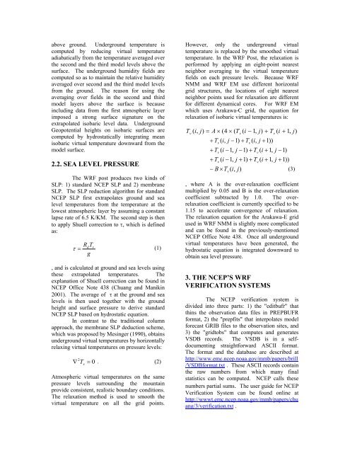
above ground. Underground temperature is computed by reducing virtual temperature adiabatically from the temperature averaged over the second and the third model levels above the surface. The underground humidity fields are computed so as to maintain the relative humidity averaged over second and the third model levels from the ground. The reason for using the averaging over fields in the second and third model layers above the surface is because including data from the first atmospheric layer imposed a strong surface signature on the extrapolated isobaric level data. Underground Geopotential heights on isobaric surfaces are computed by hydrostatically integrating mean isobaric virtual temperature downward from the model surface. 2.2. SEA LEVEL PRESSURE The WRF post produces two kinds of SLP: 1) standard NCEP SLP and 2) membrane SLP. The SLP reduction algorithm for standard NCEP SLP first extrapolates ground and sea level temperatures from the temperature at the lowest atmospheric layer by assuming a constant lapse rate of 6.5 K/KM. The second step is then to apply Shuell correction to τ, which is defined as: RdTv τ = (1) g , and is calculated at ground and sea levels using these extrapolated temperatures. The explanation of Shuell correction can be found in NCEP Office Note 438 (Chuang and Manikin 2001). The average of τ at the ground and sea levels is then used together with the ground height and surface pressure to derive standard NCEP SLP based on hydrostatic equation. In contrast to the traditional column approach, the membrane SLP deduction scheme, which was proposed by Mesinger (1990), obtains underground virtual temperatures by horizontally relaxing virtual temperatures on pressure levels: 2 ∇ T v = 0 . (2) Atmospheric virtual temperatures on the same pressure levels surrounding the mountain provide consistent, realistic boundary conditions. The relaxation method is used to smooth the virtual temperature on all the grid points. However, only the underground virtual temperature is replaced by the smoothed virtual temperature. In the WRF Post, the relaxation is performed by applying an eight-point nearest neighbor averaging to the virtual temperature fields on each pressure levels. Because WRF NMM and WRF EM use different horizontal grid structures, the locations of eight nearest neighbor points used for relaxation are different for different dynamical cores. For WRF EM which uses Arakawa-C grid, the equation for relaxation of isobaric virtual temperatures is: Tv v + T v ( i, j −1) + Tv ( i, j + 1)) v Tv i −1, j −1) + Tv ( i + 1, Tv i −1, j + 1) + Tv ( i + 1, B × Tv ( i, j) ( i, j) = A × ( 4 × ( T ( i − 1, j) + T ( i + 1, j) + ( j −1) + ( j + 1)) − (3) , where A is the over-relaxation coefficient multiplied by 0.05 and B is the over-relaxation coefficient subtracted by 1.0. The overrelaxation coefficient is currently specified to be 1.15 to accelerate convergence of relaxation. The relaxation equation for the Arakawa-E grid used in WRF NMM is slightly more complicated and can be found in the previously-mentioned NCEP Office Note 438. Once all underground virtual temperatures have been generated, the hydrostatic equation is integrated downward to obtain sea level pressure. 3. THE NCEP’S WRF VERIFICATION SYSTEMS The NCEP verification system is divided into three parts: 1) the "editbufr" that thins the observation data files in PREPBUFR format, 2) the "prepfits" that interpolates model forecast GRIB files to the observation sites, and 3) the "gridtobs" that computes and generates VSDB records. The VSDB is in a selfdocumenting straightforward ASCII format. The format and the database are described at http://www.emc.ncep.noaa.gov/mmb/papers/brill /VSDBformat.txt . These ASCII records contain the raw numbers from which many final statistics can be computed. NCEP calls these numbers partial sums. The user guide for NCEP Verification System can be found online at http://wwwt.emc.ncep.noaa.gov/mmb/papers/chu ang/3/verification.txt .
The editbufr step thins the complete observation collection contained in the Operational PREPBUFR down to just those data to be used for verification, and creates a temporary output file. The thinning saves time and space in the next prepfits step, where the most computer work is actually done. Decision for which observations to be included in the output file is based on a user-defined input control file which allows specification of time window, areal extent and observation type to be included. Each piece of observation data contains wind, temperature, height and, moisture information along with associated observation pressure, latitude and longitude to locate the observation in three-dimensions in the atmosphere. The code prepfits reads in the observations from the temporary thinned-down observation file created by editbufr, and adds background values to each piece of observation data from one or more forecasts which are valid at the time of the observations. The background values (model forecasts) are generated by horizontal and vertical bi-linear interpolation from standard pressure level output from WRF, AVN, NGM, RUC and Eta models in GRIB format. Vertical interpolation is linear in ln p for everything except specific humidity, which is interpolated as the ln of q linear in ln p. The moisture variable in PREPBUFR and PREPFITS is specific humidity q. Two options are available for verifying forecasts at shelter level. The first option is to directly compare the post-processed shelter level variables of the model (e.g., 2 meter Temperature & moisture and 10 meter winds) with observation. This method only involves a horizontal interpolation. There is no adjustment for discrepancies in the elevation of observations versus model terrain height. After all, forecasters don't do this calculation when using these fields. The second option is to perform a 3-dimensional interpolation of the postprocessed fields from the model, which always extend to 1000 mb, to the observed pressure. This option performs the necessary adjustment for elevation differences between observation and model terrain. It also reflects what the forecasters will see in the below terrain isobaric fields coming out of the model post-processor like 1000mb and even 850 mb fields under the Rockies. The code gridtobs read in instructions from a control file and generates VSDB records containing the desired partial sums that can used to calculate forecast biases, root mean square errors, and standard deviation, etc. The control file contains the bounding parameters, such as the verifying model, verifying dates, verifying observation types, verifying areas, verifying variables, and verifying levels, over which the partial sums are to be accumulated. 4. CLOSING REMARKS The verification results from WRF preimplementation test that were carried out using NCEP’s WRF post processor and verification system will be presented by Bernardet, et al. (2004). The user guides that contain information on how to download, install, and use both systems can be found at: http://wwwt.emc.ncep.noaa.gov/mmb/papers/chu ang/2/wrfpost.txt , for NCEP’s WRF post processor and http://wwwt.emc.ncep.noaa.gov/mmb/papers/chu ang/3/verification.txt , for NCEP’s verification system. 5. REFERENCE Bernardet L., Nance L., Chuang H., Loughe A., and Koch S., 2004: Verification Statistics for the NCEP WRF Pre-Implementation Test. Part I: Deterministic Verification of Ensemble Members. WRF/MM5 Joint Workshop, Boulder, Colorado, 2004. Chuang H. and Manikin G. , 2001: THE NCEP MESO ETA MODEL POST PROCESSOR: A DOCUMENTATION. NCEP Office Note No. 438, NOAA/NWS, 52 pp. The Office Note 438 is also available online at http://wwwt.emc.ncep.noaa.gov/mmb/papers/chu ang/1/OF438.html . Mesinger, F., 1990: Horizontal pressure reduction to sea level. Proc. 21st Conf. for Alpine Meteor, Zurich, Switzerland, 31-35.
Page 1: NCEP'S WRF POST PROCESSOR AND VERIF

NCEP'S WRF POST PROCESSOR AND VERIFICATION ... - MMM

Create successful ePaper yourself

Delete template?

Save as template?