MEXART: I. Sensitivity of the array and observable Inter Planetary ...

MEXART: I. Sensitivity of the array and observable Inter Planetary
Scintillation sources.
S. Jeyakumar, A. Carrillo Vargas, A. Gonzalez Esparza, E. Andrade Mascote
Instituto de Geofísica, UNAM
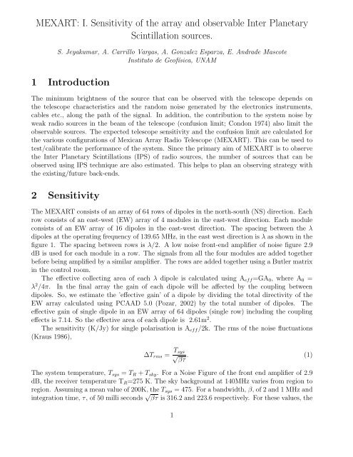
1 Introduction
The minimum brightness of the source that can be observed with the telescope depends on
the telescope characteristics and the random noise generated by the electronics instruments,
cables etc., along the path of the signal. In addition, the contribution to the system noise by
weak radio sources in the beam of the telescope (confusion limit; Condon 1974) also limit the
observable sources. The expected telescope sensitivity and the confusion limit are calculated for
the various configurations of Mexican Array Radio Telescope (MEXART). This can be used to
test/calibrate the performance of the system. Since the primary aim of MEXART is to observe
the Inter Planetary Scintillations (IPS) of radio sources, the number of sources that can be
observed using IPS technique are also estimated. This helps to plan an observing strategy with
the existing/future back-ends.
2 Sensitivity
The MEXART consists of an array of 64 rows of dipoles in the north-south (NS) direction. Each
row consists of an east-west (EW) array of 4 modules in the east-west direction. Each module
consists of an EW array of 16 dipoles in the east-west direction. The spacing between the λ
dipoles at the operating frequency of 139.65 MHz, in the east west direction is λ as shown in the
figure 1. The spacing between rows is λ/2. A low noise front-end amplifier of noise figure 2.9
dB is used for each module in a row. The signals from all the four modules are added together
before being amplified by a similar amplifier. The rows are added together using a Butler matrix
in the control room.
The effective collecting area of each λ dipole is calculated using Aeff=GA0, where A0 =
λ 2 /4π. In the final array the gain of each dipole will be affected by the coupling between
dipoles. So, we estimate the ’effective gain’ of a dipole by dividing the total directivity of the
EW array calculated using PCAAD 5.0 (Pozar, 2002) by the total number of dipoles. The
effective gain of single dipole in an EW array of 64 dipoles (single row) including the coupling
effects is 7.14. So the effective area of each dipole is 2.61m 2 .
The sensitivity (K/Jy) for single polarisation is Aeff/2k. The rms of the noise fluctuations
(Kraus 1986),
∆Trms = Tsys
√ . (1)
βτ
The system temperature, Tsys = TR + Tsky. For a Noise Figure of the front end amplifier of 2.9
dB, the receiver temperature TR=275 K. The sky background at 140MHz varies from region to
region. Assuming a mean value of 200K, the Tsys = 475. For a bandwidth, β, of 2 and 1 MHz and
integration time, τ, of 50 milli seconds √ βτ is 316.2 and 223.6 respectively. For these values, the
1

Figure 1: The block diagram of MEXART EW array of dipoles
rms noise, ∆Trms and minimum detectable flux density ∆Srms = (2k/Aeff)∆Trms are estimated
(see Table 1)
The coupling between NS elements will influence the aperture efficiency. This factor is not
known, so we use a value of 0.7 measured using Crab nebula as the aperture efficiency. This
value is used for the calculation of the effective area using the physical area, for the NS array of
rows.
3 Confusion limit
The confusion noise due to faint radio sources within the beam depends on the beam size and
the frequency. The confusion limit is defined as (Condon 1974),
Sc =
q 3−γ
3 − γ
1
1−γ
(n0Ωb) 1
1−γ , (2)
where γ and n0 are defined as, n(s)ds = n0s γ ds. Here n(s) is the differential source count. The
effective telescope beam,
Ωb = π θ1θ2
4 (γ − 1)ln(2)
2

Table 1: Expected telescope sensitivity and confusion limit for various configurations
Configuration Area Sensitivity ∆Srms ∆Srms Confusion limit
m 2 K/Jy Jy Jy Jy
(β=2MHz) (β=1MHz)
1 module 41.7 0.0151 99 140 397
1 row 167.86 0.0608 25 35 137
2 rows 205⋆ 0.074 20 29 133
4 rows 411⋆ 0.149 10 14 57
16 rows 1644⋆ 0.595 2.5 3.6 16.5
Full array 6576⋆ 2.38 0.6 0.9 5.43
⋆ Calculated by assuming an efficiency factor of 0.7.
The beam widths in two perpendicular directions are denoted by θ1 and θ2. The factor q is
usually taken to be 5. The source count at 178 MHz from the Cambridge survey provides
γ = 2.3 and n0 = 1.0 × 10 3 sources/sr. Since the operating frequency of MEXART is closer to
this frequency, the source count at 178MHz are used for the calculations. Using these values,
Sc = 4.1454(θ ′′
1 θ′′
2 )1/1.3 Jy. (3)
The confusion limit for different configurations are also listed in table 1.
4 Observable sources
For detection at 3σ level with 2MHz bandwidth, the detection limit is about 1.8 Jy. For a
spectral index of 0.75, this detection limit at 178 MHz is smaller by factor of 1.137. This yields
a detection limit of 1.6 Jy at 178MHz. The number of sources brighter than 1.6 Jy at 178MHz is
4900 (obtained using NED). Limiting the observations to elongation angles less than 45 degrees
limits the declination to ±68.5 degrees, and the number of sources observable within this range
are about 4600. Restricting the scintillation targets to elongation angles between 45 and 15
degrees, the fraction of sky covered is about 0.108. Thus the number of sources that can be
easily detected using IPS technique in a day are about 460 (see also next section).
5 IPS of radio sources
At the telescope operating frequency of 139.65 MHz, the angular size of the source that will
scintillate is about 1 arcsec. In case of extended sources, the compact components that are
smaller than 1 arcsec will scintillate. The scintillation index, m = ∆Srms/ST, where ∆Srms is
the scintillating flux and ST is the total flux of the source. For sources detected at N σ level the
lower limit to the scintillation index, m, is 1/N. For example, for a 5σ detection, scintillation
index greater than 0.2 is measurable.
The scintillation index of a point source decreases as the elongation angle (ǫ), the angle
subtended by the lines of sights to the source and the Sun from the observer, increases. The
3

Scintillation index
1
0.1
0.01
0.001
15.0 18.1 21.88
26.56
32.46
40.08
Elongation
50.6
Figure 2: Variation of scintillation index with solar elongation angle.
68.02
scintillation index, m, is related to ǫ as m ∝ sin(ǫ) −1.75 (Manoharan et al., 1995) as shown
in figure 2. A lower limit on the scintillation index sets an upper limit on the elongation angle
up to which scintillations can be measured. The lower-limit to the m and the corresponding
upper-limit to the ǫ are given in the table 2, for different detection limits.
6 Scintillation map and observing strategy
The region set by the ǫ limit above are shown in figure 3. For an integration time of 50 ms, the
minimum detectable flux is 0.6 Jy. Assuming that most of the sources are close to the detection
limit, the number of sources that would fall within each zone are given in the table 2. This is
calculated assuming that the lines of sights with elongation angles less than 15 ◦ are not observed
due to strong scattering. Since the telescope is a transit instrument, the above elongation angles
correspond to a transit time (see the table 2). During the transit time the observations can be
carried out. For a source the ON source time is about 5 mins. Assuming 10 mins of observing
time for each source including the OFF source observations, the total data-time is about 31
hours for 5σ and 34 hours for 10σ detection. To acquire the data within the transit time of the
IPS-zone the required receivers are 6 for 5 σ detection and 3 for 10 σ detection. The number
of sources that can be observed with elongation angles less than about 75 degree are about 650.
These sources can be observed using 7 receivers over a transit time of 10 hours.
4

90
>10 σ
8 σ 5σ
60
30
Figure 3: Region of the sky with the detection/scintillation index limit.
3σ
Table 2: Table of IPS-zone and the number of sources.
Observing limit m-limit ǫ-limit Number of sources Transit Time
degree Total IPS-zone (Hour)
1.8 Jy (3σ) 0.33 29 4900 230 3.87
3.0 Jy (5σ) 0.2 40 3000 310 5.3
6.0 Jy (10σ) 0.1 75 826 340 10.0
7 Conclusion
The sensitivity and the confusion limit of the radio array, MEXART are estimated. These values
are tabulated for various configurations of the array, so that comparison can be made with
observations aimed at calibrating the array. Based on the sensitivity estimates, an observing
strategy is formulated for the observations of scintillating sources.
8 References
1. Condon, J. J. 1974, ApJ, 188, 279
2. Kraus, J. D., 1986, “Radio Astronomy”, 2nd ed., Cygnus Quasar Book, Powell.
3. Manoharan, P. K., Ananthakrishnan, S., Dryer, M., Detman, T. R., Leinbach, H., Kojima,
5

M., Watanabe, T., & Kahn, J. 1995, Sol. Phys., 156, 377
4. Pozar M. D., 2002, PCAAD 5.0: Personal Computer Aided Antenna Design, Inc. Leverett,
MA.
6