Changes in Mutual Fund Flows and Managerial Incentives

Changes in Mutual Fund Flows and Managerial Incentives
Min S. Kim ∗
University of New South Wales
December 1, 2010
Abstract
I show that the shape of the relationship between mutual fund flows and past performance
varies over time. In particular, flows become less sensitive to high performance following periods
of volatile markets and following periods of less dispersion in performance across funds. As a
result, during the 2000s, when both effects are present, the flow-performance relationship is not
convex. Moreover, I show that underperforming managers engage in less risk-shifting towards
the end of the year when markets are volatile and performance is less dispersed across funds.
These results are consistent with the view that investors’flows respond more to performance
when it is more informative and that fund managers anticipate this variable flow response.
JEL Classification Codes: C14, G10, G20, G23
Keywords: mutual funds, flow-performance relationship, risk-shifting
∗ School of Banking and Finance, Australian School of Business, University of New South Wales, email:
min.kim@unsw.edu.au. I thank Stephen Brown, Daniel Carvalho, George Cashman (discussant), Christopher Clifford
(discussant), Harry DeAngelo, Wayne Ferson, Christopher Jones, Aneel Keswani (discussant), Diana Knyazeva, John
Long, Tim Loughran, Pedro Matos, Rosa Liliana Matzkin, Kevin Murphy, Oguzhan Ozbas, Raghavendra Rau, Antoinette
Schoar, Clemens Sialm, David Solomon, Kumar Venkataraman, Jerold Warner, Mark Westerfield, William
Zame, and participants at the EFA aanula meetings in Frankfurt, the FIRS conference in Florence, the FMA annual
meetings in Reno and at the finance seminars at Drexel University, Hong Kong University of Science and Technology,
INSEAD, National University of Singapore, Rutgers University, University of New South Wales, University of Notre
Dame, University of Rochester, and University of Southern California for their helpful comments. I am especially
grateful to my advisor Wayne Ferson, Christopher Jones, Mark Westerfield, and William Zame for valuable discussions
and suggestions. All errors are my own.

An important issue in the agency literature is the incentive effects of compensation structures
on agents’real behavior. In the mutual fund industry, given that fees are proportional to assets
under management, the relationship between money flows and past performance can induce implicit
performance compensation. Brown, Harlow, and Starks (1996) and Chevalier and Ellison (1997)
argue that convexity in the relationship provides managers who are behind the markets (or their
peers) with incentives to take more risk towards the end of the year. These actions are undertaken
in an attempt to improve performance and thereby increase inflows in the following year. Given
that the implicit payoff looks like a call option, underperforming managers may engage in such
risk-shifting even at the expense of investors’interests. 1
This paper examines whether managers respond to the incentives provided by this implicit
compensation scheme. To this end, I look at how their risk-shifting varies according to the shape
of the relationship between net flows and past performance (e.g., benchmark-adjusted returns in
the prior year). I show that contrary to the common view in the literature that the relationship is
convex, its shape depends on conditioning variables, particularly market volatility and performance
dispersion across funds. I then study manager’s risk shifting as it relates to time variation in the
shape of the flow-performance relationship.
I first show that the flow-performance relationship varies over time. I find that the shape
of the relationship is less convex when stock markets are volatile and when performance is less
dispersed across funds. In particular, the sensitivity of flows to high performing funds decreases
following periods of high-volatility markets and following periods of low performance dispersion.
Controlling for market volatility and performance dispersion, we cannot reject the hypothesis that
1 Earlier studies that document the convex flow-performance relationship include Ippolito (1992), Goetzmann and
Peles (1996), Gruber (1996), Chevalier and Ellison (1997), and Sirri and Tufano (1998). In the models of Starks
(1987) and Panageas and Westerfield (2009), option-like incentive fees can lead to managers’risk-seeking behavior.
Koski and Pontiff (1999) argue that fund managers use derivatives to manage unexpected cash flows rather than to
take more risk in an attempt to increase expected flows. Busse (2001) and Elton et. al. (2009) find different results
than those in Brown, Harlow, and Starks, when using daily return and monthly holding data respectively.
1

flows are linearly related to performance. Such variations lead to an alteration in the shape of
the flow-performance relationship in the 2000s. Consistent with earlier studies, it is convex from
1983 to 1999, but it is not convex during the highly volatile market conditions of the early 2000s.
In addition, managers’ risk-shifting behaviors tend to differ according to these two conditioning
variables: performance dispersion and market volatility. When the expected shape of the flow-
performance relationship conditional on those variables is not convex (i.e., when performance is
less dispersed and when markets are more volatile), underperformers do not engage in risk-shifting.
As a result, in the 2000s, managers performing worse than the markets tend to reduce risk- shifting.
My results are consistent with the view that investors’flows respond more to performance when it
is more informative and that fund managers anticipate this variable flow response.
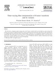
Figure I. Flow-performance relationship and 90% confidence interval
The y-axes represent expected annual net flows into and out of nonindex funds from 1983 to 1999
(before 2000) and from 2000 to 2008 (after 2000). Performance is annual returns minus the CRSP value
weighted index (CRSP VW). The expected annual net flows are estimated using kernel regressions suggested
by Robinson (1988) after controlling for contemporaneous performance, the second lag of performance, age,
size, expense ratio, volatility, and lagged flow of funds, industry flow, and style flow. See Table I for the
variable description. Funds are aggregated across share classes, excluding institutional share classes. The
total number of funds is 2,264 over 1983 to 2008 and the numbers of observations are 6,771 and 10,908 before
2000 and after 2000 respectively.
expected annual net flows
0.5
0.4
0.3
0.2
0.1
0
­0.1
­0.2
before 2000
after 2000
­0.25 ­0.2 ­0.15 ­0.1 ­0.05 0 0.05 0.1 0.15 0.2 0.25
lagged return over the market value­weighted index
2

I estimate the relationship between fund flows and excess returns over the markets from 1983
to 1999 and from 2000 to 2008 respectively, using kernel regression (Figure I). After controlling for
the effects of fund characteristics and money flows to the mutual fund industry as a whole, I find
substantial decreases in convexity in the recent period. In particular, the marginal flow to high
performing funds does not increase with performance. As a consequence, a fund outperforming the
market value-weighted index by 20% attracted annual net flows of 30% prior to 2000 on average
but only 10% in the subsequent decade. 2 Given the average fund sizes of $1 billion and $1.4 billion
during those periods, respectively, this type of fund had annual net inflows of $300 million prior
to 2000 on average, but only $140 million after that. Ordinary least square (OLS) regressions also
confirm these changes. The coeffi cient on squared performance decreases from 0.6 to -0.3 after
2000, which suggests a change from a convex to a concave relationship (when the relationship is
increasing, the predominant difference in marginal flow for high performance can be captured by
convexity or concavity). I also find similar decreases in convexity using ranking as performance
measure. 3
I show that time-variation in the flow-performance sensitivity (expected marginal flow) con-
tributes to the concave shape in the 2000s. Throughout the period from 1983 to 2008, the flow-
performance relationship is concave following periods of highly volatile markets, whereas it is convex
following periods of low-volatility markets. I also find that the shape is more convex when per-
formance is more dispersed across funds (after controlling market volatility). For example, 10% of
performance dispersion reduces the concavity in highly volatile markets by around half.
2 The changes in the flow-performance relationship are predominant for high performance, not for low performance.
This can be explained by the findings that the (net) flow-performance relationship arises from the responses of inflows
to past performance and outflows are unrelated to past performance (see Bergstesser and Poterba (2002), O’Neal
(2004), Johnson (2007), and Ivkovic and Weisbenner (2009)).
3 Using ranking of raw returns as a performance measure, I also find a substantial decrease in marginal flow to
top-ranked funds in the post-2000 period. Performance dispersion increases convexity of the relationship between
net flows and performance ranking, but market volatility appears statistically insignificant for the relationship. See
Section III.C for the details.
3

These results are consistent with the predictions in Berk and Green (2004) and Kim (2010)
that the marginal flow to high-performing funds is low when performance is less attributable to
skills. In both models, investors use past performance– represented as skills plus noise– as an
inference of managers’abilities (and efforts). When performance reflects more luck relative to skill,
the sensitivity of flows to superior performance is low. The contribution of skills to performance
increases with cross-sectional variation in skills but decreases with variation in noise. As a result,
when skills are less heterogeneous across managers and when performance appears noisier, investors
become less responsive to high performance. 4
Changes in risk-shifting behavior are consistent with the view that managers respond to the
incentives provided by the implicit performance compensation. Given the changes in the shape of
the flow-performance relationship, I examine variations in the relationship between performance
and risk-shifting. Low-performing funds typically take more risk in the fourth quarter, but this
risk-shifting is significantly reduced after 2000, decreasing by about 70%. The same variables
that determine the shape of the flow-performance relationship also explain these changes. After
conditioning the relationship between performance and risk-shifting, I find that managers who are
behind the markets tend to increase risk in the fourth quarter when performance in the middle of
the year is more dispersed across funds. In periods when performance dispersion is low, it is the
high-performing managers who engage in such risk-shifting. I also show that low-performing funds
tend to take more systematic risk in the rest of the year when market volatility up to the third
quarter is low.
The main contribution of the paper is to propose a conditional relationship between flows
4 In the model presented in Kim (2010), there is no intrinsic shape in the flow-performance relationship. Rather, in
equilibrium, incentive fees depend on the likelihood that the manager has high skills and actively manages the fund
relative to the likelihood that she follows a passive index strategy. Thus, the shape can be convex, linear or concave.
Del Guercio and Tkac (2002) find a symmetric relationship for pension funds, and Kaplan and Schoar (2005) find a
concave relationship for private equity funds.
4

and performance 5 and to document changes in managers’risk-shifting behavior according to the
expected shape of the relationship. In particular, I show that flows are less responsive to high
performance when markets are volatile and when performance is less dispersed across funds in the
prior period. These variations lead to nonconvexity in the relationship in the 2000s. On the other
hand, Huang, Wei, and Yan (2005) and Sigurdsson (2005) find that in the 1990s, flows become
more sensitive for middle (and low) performance, leading to a more linear relationship between
flows and performance, than in the 1980s.
In addition, this paper makes several contributions. First, my findings provide an explanation
for the recent growth in passive management in the mutual fund industry, such as closet-indexing.
Managers face fewer incentives to engage in active management because of lower marginal flow
to high-performing funds. As suggested in Kim (2010), managers track market indexes when
performance-based compensation for active funds is low. Second, while investors are less attracted
to superior performance in the 2000s, fund flows are negatively related to expense ratios. I find
that funds with high expense ratios had more inflows before 2000 (see also Barber, Odean, Zheng
(2005) and Huang, Wei, and Yan (2005)). Yet, after 2000, my results show that a 1% increase in
the ratios led to a 3-5% decrease in net flows. This is consistent with recent anecdotal evidence that
past performance is no longer the most important factor, whereas fees have become critical when
investors choose mutual funds. According to a survey by the Investment Company Institute in
2006, more investors consider fees rather than past performance (see “Investors Flock to Low-Cost
Funds,”J. Clements, 2007, The Wall Street Journal). As discussed in Appendix, the negative effect
of expense ratios after 2000 seems to be associated with a decrease in 12b-1 fees, most of which are
used to compensate financial advisers. Finally, my results are consistent with investors attempting
to distinguish skills associated with active management from a passive index strategy. I find that the
5 Olivier and Tay (2009) and Wang (2009) show that contemporaneous GDP growth affects the flow-performance
relationship. My paper uses lagged variables to form a conditional expectation about the shape of the relationship.
5

flow-performance relationship is insignificant for index funds in most cases (see also Elton, Gruber,
and Busse (2004)). Nonetheless, index fund flows seem to increase with performance compared to
the funds with the same value and size characteristics. Given that outperforming those peer funds
requires more than passive management, the results are consistent with the view that investors chase
good performance because they perceive that it represents skills (e.g., Gruber (1996) and Zheng
(1999)). Also, the changes in the flow-performance relationship according to market volatility and
performance dispersion that I document seem less supportive of a story where investors irrationally
chase recent winner funds (e.g., Sapp and Tiwari (2004)). 6
Section I and II discuss methodologies and results for changes in the flow-performance relation-
ship and changes in managers’risk-shifting respectively. I present the results of robustness check
in Section III and conclude in Section IV.
I. Flow-performance relationship
A. Data and variable description
I obtain market indexes and mutual fund data from Morningstar, including returns, total net
assets (TNA), 9 style categories (value and size), index fund flags, and funds’benchmark indexes
as disclosed in fund prospectuses. I aggregate across share classes based on their TNA. 7 Market
returns are proxied by the Center for Research in Security Prices value-weighted (CRSP VW) index.
My sample covers all U.S. equity mutual funds, excluding index funds (according to fund
prospectuses), sector funds, specialized funds and international funds, from 1983 to 2008 annually
(data starts in 1980 to obtain lagged variables). To compare my results with Chevalier and Ellison
6 I also find that in the areas where hedge funds are concentrated (New York and Boston), marginal flow to high
performing funds decreases more compared to other areas after 2000. The market share of the funds (whose managers
are) in those areas decreases from 50% in 1999 to 30% in 2008. These results can support a view that flows are less
sensitive to high-performance because skilled managers leave the industry (e.g., a brain drain to hedge funds; see
Kostovetsky (2007) and Massa, Reuter and Zitzewitz (2009)).
7 I obtained similar results using the CRSP data. Using only Morningstar increases the sample size (no crossidentification
between two data sets) and better aggregates across share classes.
6

(1997), I follow their sampling criteria. I remove small funds (assets less than $10 million) and
young funds (less than 3 years old) as of the beginning of the period over which fund flows are
measured. 8 I also exclude the funds that are closed to new or all investors in their closing years
and afterwards (See Bris et. al. (2007) for a detailed discussion about fund closures), institutional
share classes, funds that acquire other funds in their merger years, and the funds that are liquidated
within 6 months before the date that fund flows are measured.
Fund flows are measured annually at the end of December and lagged performance over the
preceding calendar year. I define fund flows as a percentage change in TNA, net of capital gains
and dividends from investments. I measure net flows of a fund i at year t by
net flowi,t = T NAi,t − T NAi,t−12
T NAi,t−12
where ri,t is the fund’s return over the period from t − 1 to t. 9
− ri,t
Following Chevalier and Ellison (1997), I measure performance as excess returns over CRSP
VW returns. Since I focus on investors’reactions to performance, I also use simple performance
measures that may be readily available to investors. In particular, relative returns compared to
benchmark indexes or to the S&P500 index are available on fund companies’websites or financial
websites such as Yahoo! Finance. Del Guercio and Tkac (2002) show that excess returns over market
indexes, such as the S&P500 index, are important determinants of mutual fund flows. They also
provide evidence that mutual fund flows are related to factor-adjusted performance measures as the
sophisticated measures are correlated with readily available measures. When a fund’s benchmark
index is missing, I use the most frequently used benchmark by other funds with the same styles
8 Young funds may go through an incubation process. Chevalier and Ellison (1997) include funds between two and
three years old. I exclude them since I also use lagged flows as a control variable. Results are similar if I include
them.
9 To avoid effects due to measurement errors or extreme observations, I winsorize fund flows at 1% and 99% levels
following Barber, Odean and Zhang (2005). My results do not depend on those outliers.
(1)
7

(Sirri and Tufano (1998) use relative returns compared to the funds with the same investment
objectives). Finally, I also compute average returns on equity funds in the same style categories
(peer funds), which I call style returns. Relative returns compared to style returns is likely to be
important if investors select funds based on value and size characteristics and make comparisons
among funds within the same style category. To summarize, I use four performance measures
depending on benchmark returns: CRSP VW, S&P500 index, the fund’s benchmark index, and
style returns.
Other variables used in the regressions include fund size, age, expense ratios and volatility.
Many studies find that a small fund and a young fund grow faster (e.g., Chevalier and Ellison
(1997), Sirri and Tufano (1998), Del Guercio and Tkac (2002), and Barber, Odean and Zhang
(2005)). I measure size as the natural logarithm of ratio of a fund’s TNA to the average TNA of all
equity funds in the sample at the beginning of each year (using the level could make the variable
nonstationary). I use log age, which is the natural logarithm of the number of months since the
inception dates. I also include expense ratios in the regression. Expense ratios do not include load
fees (Morningstar does not provide historical load fees; using the CRSP data, I add one-seventh of
load fees, as Sirri and Tufano (1998) suggest, and obtain similar results). Some studies find that
fund flows are negatively related to volatility of past returns. I measure volatility as the standard
deviation of monthly returns over the prior two years (see Barber, Odean and Zheng (2005)).
I also control for net flows to the industry (all equity mutual funds in the CRSP database)
as a whole since they could influence flows to individual funds. Industry flow can also handle
fixed time effects if any. Cooper, Gulen, and Rau (2005) find that investors chase styles and funds
could attract more inflows after changing their names to reflect popular style characteristics– even
without actual changes in investment styles– over 1994 to 2001. Thus, I also include style flows (net
flows to funds with specific size and value characteristics according to the Morningstar categories)
8

in the regressions. I add contemporaneous performance, and the second lag of performance to
examine whether investors consider less recent performance. To control for fund fixed effects, I use
lagged flows.
My sample includes 17,679 observations (fund and year) for 2,264 funds from 1983 to 2008.
They account for 83% of net assets of nonindex funds on average. I conduct a separate analysis
before and after 2000, around which the markets and the money management industries seem to
have changed. In early 2000s, the dot-com bubble burst and markets were highly volatile. Also,
hedge funds experienced sharp growth. According to Hennesse Group LLC, total net assets of
hedge funds increased by 50%, from $221 billion in January 1999 to $324 billion in January 2000.
From 1998 to 1999, the growth rate was only 6%. The observations are 6,771 and 10,908 for the
pre-2000 and the post-2000 periods respectively. 10
Table I presents descriptive statistics. Over 1983 to 2008, nonindex funds have annual inflows
of around 10% on average. Before 2000, the average fund flows are 13%, which decrease to 9%
after 2000. Yet, the decrease is not statistically significant (the t-statistics for the equal means are
adjusted for correlations among funds and across years). The average total net assets are about
$1 billion before 2000 and grow to $1.4 billion after 2000. Due to the introduction of new funds in
recent years, the average fund is younger after 2000. The average expense ratios are slightly higher
by 0.05% after 2000. The standard deviations of monthly returns are similar in the subperiods,
around 4.3%. Industry flows and style flows are fewer in the 2000s. The mutual fund industry had
net inflows of 9% over 1983 to 1999, which decreased to 4%, after 2000 (the difference is significant).
The average net flows to styles are around 10% before 1999 but only 4.7% after 2000.
The sample composition of funds does not have dramatic changes in age, size and style around
2000 as shown in Figure II. I define young funds and small funds as those funds below the median
10 There is also a dramatic change in the time-series of the flow-performance relationship around 2000 (Section I.E
and Figure 5 (a)). Using the year 1999 or 2001, I obtained similar results.
9

age (10 years) and size ($0.3 billion) respectively. Panel (A) illustrates that the proportion of large
funds increased dramatically in the 1990s. The proportion of young and old funds has been stable
since early 1990s (Panel (B)). Moreover, the composition of fund styles is also similar throughout
the years.
B. Kernel regression methodology
I use the semi-nonparametric estimation suggested by Robinson (1988). Chevalier and Ellison
(1997) use this procedure for the flow-performance relationship but also examine the sensitivity
differences across fund age groups. They show that flows to old funds (5 years old or more) are
less sensitive to performance. Yet, the differences do not appear statistically significant. Thus, I
estimate the flow-performance relationship for funds of any age, controlling age effects by an age
variable in the regressions. I use a panel of funds and year and estimate
net flowi,t = g(performancei,t−1) + β 3performancei,t + β 4performancei,t−2 + β 5age i,t−1
+β 6size i,t−1 + β 7expensei,t−1 + β 8volatilityi,t−1 + β 9industryi,t
+β 10stylei,t + β 11net flowi,t−1 + εi,t, (2)
where the variables are described in the preceding section. The error term is orthogonal to perfor-
mance as E[εi,t|performancei,t−1] = 0. I estimate the function g(performancei,t−1) using kernel
regressions. I choose optimal bandwidths by the cross-validation method, which improves effi ciency
despite its computational costs (see Appendix). Previous studies do not use the cross-validation
method (e.g., Chevalier and Ellison (1997) and Sensoy (2009)).
As Robinson (1988) proves, we can obtain √ n-consistent and unbiased estimates for β 3 to β 11
in the Equation (2) by the following steps: (a) Run each kernel regression of net flows and the
10

control variables against lagged performance to obtain their expected values conditional on lagged
performance; (b) Run OLS regressions of residual net flows on the residual control variables, defined
as actual values minus expected values obtained from (a), to estimate β 3 to β 11 (Frisch-Waugh-
Lovell theorem). Using the estimates β 3 to β 11, I can obtain net flow ∗ i,t by
net flow ∗ i,t = net flowi,t − ( β 3performancei,t + β 4performancei,t−2 + β 5age i,t−1
+ β 6size i,t−1 + β 7expensei,t−1 + β 8volatilityi,t−1 + β 9industryi,t
+ β 10stylei,t + β 11net flowi,t−1). (3)
To estimate g(·), I run kernel regressions of net flow ∗ i,t against performancei,t−1. This func-
tion has the interpretation, E[net flow ∗ i,t |performancei,t−1] = g(performancei,t−1). In words, I
estimate the flow-performance relationship as expected fund flows conditional on past performance,
controlling other factors, such as industry growth, size, and age. One limitation of this method is
its inability to identify α because the regression Equation (2) is (observationally) equivalent to
net flowi,t = α ∗ + g(performancei,t−1) + α − α ∗ ...
Therefore, I normalize g(performancei,t−1) so that we have g(0) = 0.
To account for correlations among funds and autocorrelations over time, I report standard
errors after clustering observations by year and fund.
C. Linear regression methodology
I run OLS regressions of net flows on each performance measure and the control variables, after
assuming that g(·) in Equation (2) is quadratic in lagged performance. Previous studies also use
the square of lagged performance to capture nonlinearity of flow-performance relationships (e.g.,
11

Barber, Odean and Zheng (2005) and Sensoy (2009)). I run the following regressions using panel
data:
net flowi,t = α + β 1performancei,t−1 + β 2performance 2
i,t−1
+β 3performancei,t + β 4performancei,t−2 + β 5age i,t−1 + β 6size i,t−1
+β 7expensei,t−1 + β 8volatilityi,t−1 + β 9industryi,t + β 10stylei,t
+β 11net flowi,t−1 + εi,t, (4)
where the variables are the same as in the Equation (2). Similar to kernel regressions, I report
standard errors after clustering by year and fund.
D. Changes in the flow-performance relationship
I first present the kernel regression results for the two subperiods. Figure III shows the esti-
mates of the flow-performance relationship, i.e., the function g(performancet−1) in Equation (2),
along with their 90% confidence intervals in each period. For all four performance measures, the
striking changes are in shapes: convexity before 2000 and linearity or concavity after 2000. In par-
ticular, expected inflows after good performance are much fewer after 2000 than before that year,
and the decreases in expected inflows are larger for higher performance. For example, expected
inflows after outperforming the CRSP VW by 10% are 14.3% before 2000, but they decrease to
6.6% after 2000. Net inflows to funds with 20% outperformance decreased from 27.8% to 9.4%.
On the other hand, the flow-performance relationship for poor performance are similar between the
two periods. Table II presents the coeffi cients on the control variables (the linear part in Equation
(2)).
12

The most dramatic changes are for performance relative to peer funds with the same styles. As
shown in Figure III, the sensitivity of the relationship (i.e., the slope of the function g(performancet−1))
is sharply increasing with the performance before 2000. Yet, after 2000, the sensitivity declines.
For instance, for 10% outperformance relative to peer funds, the sensitivity is around 3.6 before
2000 but only 1.1 after that.
The shape of the relationship between fund flows and excess returns over styles is odd for the
performance region less than -20% or more than 20% prior to 2000. This is because there are not
many data points at those extremes. The 5 percentile and 95 percentile of excess returns over style
returns are around -13% and 12% respectively (other performance measures are almost -20% and
16% respectively).
The results from the OLS regressions are similar. I only report the results for performance
relative to the CRSP VW index and for performance relative to style returns since using the
S&P500 index and funds’benchmark indexes lead to almost the same results as using the CRSP
VW index and style returns respectively. Table III shows the estimates followed by standard errors
(clustered by year and fund) and p-values for each independent variable. The dependent variable is
net flows. One of the striking differences is for the slope estimates on square of lagged performance.
They are positive in the pre-2000 period but decrease to around -0.3 ∼ -0.4. The differences of
those coeffi cients are significant at 1% significance level (the test is whether the interaction term
between the squared performance and the second period dummy is zero). The estimates on lagged
performance are positive in both periods but the magnitudes are a bit smaller after 2000. I plot
the estimated flow-performance relationship (the quadratic function) in Figure IV (A).
Since the sensitivity of flow-performance relationship is given by the first derivative of the
13

Equation (4) with respect to performance,
β 1 + 2β 2performance t−1, (5)
the estimates suggest that the sensitivity changes, for example, from 1.5 + 1.3performance t−1
to 0.9 − 0.6performance t−1 when performance is excess returns over CRSP VW. Figure IV (B)
illustrates these changes in sensitivity by plotting the sensitivity as a function of past performance
(i.e., Equation (5)) before 2000 and after 2000. For all four performance measures, the sensitivity
increases with past performance before 2000 (convexity), but it decreases with past performance
after that (concavity). Yet, the most dramatic changes are for performance relative to peer funds
with the same styles, which are consistent with the kernel regression results. The sensitivity for
10% outperformance is around 2.5 on average from 1983 to 1999 but decreases to around 1 in the
post-2000 period.
Another difference between the two periods is that net flows are positively related to expense
ratios of funds before 2000 but negatively related to that after the year. Both kernel regressions
(Table II) and OLS regressions (Table III) show these contrasting impacts of expense ratios. For
example, as shown in Table III, when measuring performance compared to the CRSP VW index,
a 1% increase in expense ratios leads to a 8% increase in net flows in the following year on average
from 1983 to 1999. After 2000, expense ratios have negative impact on fund flows. A 1% increase in
expense ratios loses around 3% of net flows in the following year. Barber, Odean, Zheng (2005) and
Huang, Wei, and Yan (2005) also find a positive effect of (operating) expense ratios– not including
front-end loads– on fund flows for sample periods before 2000. Barber, Odean, and Zheng argue
that investors pay less attention to ongoing operating expenses that are embedded in fund returns
than front-end load fees. Rather, they are even attracted to funds with higher marketing expenses,
14

leading to a positive relationship between expense ratios and fund flows. I discuss variations in the
effect of the expense ratio on fund flows in Appendix.
Coeffi cients estimates for other variables have the same signs in both periods (Table II and
Table III; results for other performance measures are available upon request). For example, smaller
funds or younger funds grow more, consistent with earlier studies. A fund with less volatile returns
over the last two years attracts more inflows. Funds with more popular style characteristics received
more in the pre-2000 period. However, style flows appear insignificant in the post-2000 period when
performance is measured relative to CRSP VW (or S&P500 index). In essence, investors seem to
chase funds that outperform the markets irrespective of their styles in the 2000s.
E. Determinants of sensitivity of the flow-performance relationship
I showed that the flow-performance relationship changes around 2000. In particular, substantial
changes are marginal flow with respect to performance (i.e., the slope of g(performancet−1) or
Equation (5)). For example, Figure IV (B) shows that marginal flow increases with performance
before 2000 but decreases after 2000. Thus, I investigate what impacts the sensitivity of the flow-
performance relationship. I focus on market- or industry-wide factors, rather than fund-specific
ones, to examine variations in the sensitivity through time.
To this end, I look at how β 2 in Equation (5) changes, more specifically, how it varies depending
on market- or industry-wide conditions. Assuming linearity, I estimate
β 1 + 2β 2,tperformance t−1 = β 1 + 2(γ + δ ′ Zt)performance t−1, (6)
where Zt is a vector of conditioning variables that are known at time t. Since the Equation (6)
is the first derivative of the regression Equation (4), I run the following regression over the whole
15

sample period, including the interaction terms between those variables and squared performance
net flowi,t = α + β1performancei,t−1 + γperformance 2
+ δ′ Zt ∗ performance i,t−1 2
i,t−1
+β 3performancei,t + ...... + β 11net flowi,t−1 + εi,t. (7)
To motivate market volatility as a market-wide variable, I present in Figure V (A) the cross-
sectional estimates on the square of excess returns relative to the CRSP VW (i.e., β 2 in Equation
(4)) along with their 10% confidence intervals, and lagged market volatility (annualized standard
deviation of the daily CRSP VW returns). The estimate on the square term dramatically decreases
in 1998 and becomes negative in 2000, suggesting convexity in the flow-performance relationship.
The estimate and the lagged market volatility have almost the opposite patterns through time.
While the estimates in the first period (1983-1999) and in the second period (2000-2008) are positive
and negative respectively, there have been some periods with negative coeffi cients before 2000 and
positive coeffi cients after 2000, which seem to depend on market volatility. For instance, after the
1987 market crash, the estimate on squared performance significantly drops in 1988. Following the
less volatile markets in 2005 and 2006, the slope estimates increase in 2006 and 2007.
These results are consistent with the predictions that marginal flow to superior performance
is low when performance is noisy (Berk and Green (2004) and Kim (2010)). Figure V (C) shows
performance distributions. In low-volatility markets (less than 10%), funds underperform markets
on average, and outperformance is rare: The mean and the skewness of excess returns relative
to the CRSP VW are -3% and -0.03 respectively. When markets are highly volatile (more than
16%), funds outperform the markets on average (3%) and the performance is skewed to the right
(skewness 0.7). Thus, performance tends to improve and appears noisier in highly volatile markets.
I also look at how the sensitivity of the flow-performance relationship depends on heterogene-
16

ity in skills. To obtain a proxy for that, I first regress the cross-sectional standard deviation of
performance on the market return and the market volatility (the mean and the standard deviation
of daily returns on the CRSP VW index respectively). Given that performance is represented as
skills plus noise, its variance is the sum of the variance of skills and the variance of noise. Provided
that the variance of skills is uncorrelated with market conditions, only the variance of noise depends
on market conditions. Thus, I use the regression residual, which I call performance dispersion, as
a conditioning variable.
In addition to market volatility and performance dispersion, I use industry flow as conditioning
variables. Industry flow is the same variable used in the previous regressions. Since indicator
variables are easy to interpret (e.g., high- and low-volatility markets), I rank market return, market
volatility and industry flow into three groups respectively and assign values of -1 (low), 0 (medium),
and +1 (high). Approximately, the medium volatility is between 10% and 16%; the medium return
between 2% and 20%; and the medium industry flow between 3% and 9% (the conclusions do not
change if I use their levels, or if I use dummies for high- and low-volatility markets). High volatility
and low industry flow are prevalent in the 2000s. Figure V (B) shows the market volatility indicator
and performance dispersion.
The results are provided in Table IV (the results for performance relative to S&P500 index
are similar to Panel (A), and those for performance relative to the benchmark index are similar
to Panel (B)). Before discussing the main regressions, I first present some benchmark cases. The
first regression pools all years. The slope estimates on squared performance from 1983 to 2008 are
negative and significant for all four performance measures, suggesting the concave flow-performance
relationship on average over the whole period. The concavity effect in the second period dominates
because there are more observations after 2000. The effect of expense ratio appears negligible
since its contrasting impacts in two subperiods are cancelled out each other over the entire sample
17

period. When adding lagged flows (the second regression), the adjusted R-squared increases by
around 7-8% while most estimates change little, except expense ratios. I include lagged flows in
the rest of regressions.
Consistent with the results in Table II, using the second period dummy variable changes the
estimates on squared performance and expense ratios dramatically (the third regression). The flow-
performance relationship before 2000 appears convex but become concave in the second period. The
expense ratios are positively related to fund flows over 1983 to 1999 but have a negative impact in
the 2000s. These results are similar for all performance measures.
I now discuss the main regressions that examine the determinants of the flow-performance
sensitivity. When including the interaction terms between squared performance and lagged stock
market indicators (the regression (4)), the coeffi cients on those terms are negative (market returns
appear insignificant for the sensitivity). Note that the estimates on squared performance are statis-
tically insignificant. We cannot reject that in the medium volatility markets, the flow-performance
relationship is linear. In periods following highly volatile markets, the coeffi cient on the squared
excess returns over the CRSP VW decreases by around -0.9, which indicates concavity in the flow-
performance relationship. In low volatility markets, the coeffi cient increases by +0.9, which implies
convexity in the relationship (see Figure VI). 11 I interpret these results as supporting evidence that
investors become less responsive to superior performance in highly volatile markets because they
perceive performance arising primarily from luck.
After adding performance dispersion (uncorrelated with market volatility and returns) as a
conditioning variable (regression (5)), I find that a 1% increase in the cross-sectional standard
deviation in performance increases the coeffi cient on squared performance by around 7%. Thus,
investors appear more responsive to superior performance when performance is more dispersed.
11 When using dummy variables for market volatility, I find consistent results that convexity decreases in highly
volatile markets (see Section III.A for details).
18

Provided that performance dispersion can proxy for heterogeneity in skills, high dispersion indicates
that performance is more attributable to skills.
Industry flow appears to increase the sensitivity of the flow—performance relationship (regres-
sion (6)). This can suggest that more money in mutual funds actually goes to high-performing
funds. Provided that fund performance exhibits decreasing returns to scale (Chen et. al. (2004)),
investors invest in funds with higher expected returns when they invest more. The last regressions
show the results including all conditioning variables. Market volatility and performance dispersion
remain significant when measuring performance relative to style returns. Yet, when the CRSP
VW is used as the benchmark, market volatility becomes insignificant. This could be due to the
significant correlation between market volatility and the second period dummy.
II. Managerial incentives
I examine whether managers change their risk-shifting according to variations in the flow-
performance relationship. Brown, Harlow and Starks (1996) and Chevalier and Ellison (1997)
show that some mutual fund managers increase the riskiness of their funds toward the end of
the year as a result of the incentives provided by the flow-performance relationship. They also
argue that the increase in the riskiness is positively related to expected net flows in the following
year. Given a decrease in fund flows to outperforming funds in the 2000s, managers should engage
in less risk-shifting. In addition, variation in risk-shifting according to performance up to the
third quarter should be also different in the 2000s. When the sensitivity of the flow-performance
relationship is larger for high performance than for low performance, underperforming managers
have proper incentives to increase the riskiness of their funds while good performers lock in their
gains. Otherwise, managers who are behind the markets would have fewer incentives for such
risk-shifting. Therefore, I also look at how performance up to the third quarter affects risk-taking
19

ehavior in the fourth quarter depending on variations in the flow-performance relationship.
I measure the riskiness of funds equity holdings rather than fund returns. Busse (2001) obtain
different results than those in Brown, Harlow and Starks (1996) when using daily returns instead of
monthly returns. Thus, I examine risk measures that use holding data, such as those suggested by
Chevalier and Ellison (1997) and Huang, Sialm and Zhang (2009). Chevalier and Ellison’s measure
compares fund risk at the end of December and at the end of September. Huang, Sialm and Zhang’s
measure compares fund risk with a long term risk level, namely, over the prior 36 months.
A. Data and variable description
I use the Thomson-Reuters Mutual Fund Holdings for equity holdings and the CRSP Survivor-
Bias-Free US Mutual Fund for TNA and monthly returns (Morningstar does not provide historical
holding data). I include only the funds with the objective codes of aggressive growth, growth or
growth and income, as provided by the Thomson-Reuters. I exclude index funds by fund name,
small funds (less than $10 million at the end of September) and young funds (fewer than 2 years).
The sample period is from 1983 to 2008.
The first risk measure uses volatility of excess returns over the CRSP VW. It decomposes the
volatility into two parts (Chevalier and Ellison (1997)):
var(ri − rm) = var(ri − β irm) + (β i − 1) 2 var(rm),
where ri is the fund i’s return, rm the market return proxied by the CRSP VW index, and β i is the
fund i’s CAPM beta. Total risk, unsystematic risk and systematic risk, are defined as their square
roots, ST D(ri − rm), ST D(ri − β irm), and |β i − 1| respectively.
Risk-shifts are the risk difference between September and December, denoted by RISKDec −
RISKSep for total risk, unsystematic risk and systematic risk. To estimate RISKSep and RISKDec,
20

I construct two portfolios that hold the stocks in the fund at the end of September and December
respectively and calculate the volatility of those hypothetical portfolios using daily return data
in the prior year. As Chevalier and Ellison point out, RISKDec − RISKSep does not depend
on changes in market conditions but only on changes in equity holdings in the fourth quarter.
To estimate total risk ST D(ri − rm), I use the (annualized) standard deviation of daily excess
returns on the hypothetical portfolio over the CRSP VW returns. Likewise, unsystematic risk,
ST D(ri − β irm), is the (annualized) standard deviation of ri − β irm where β i is the beta of the
portfolio. One disadvantage of this measures is that betas of individual stocks should be estimated.
I only consider the funds of which hypothetical portfolios have 80% of funds’TNA.
Another measure is suggested by Huang, Sialm and Zhang (2009). It represents how much
riskier the fund would have been if it had held the current assets over the prior 36 months. It
measures the difference between the standard deviation of returns on a hypothetical portfolio that
holds the current assets of the fund and the standard deviation of actual returns on the fund over
the prior 36 months: hypothetical risk − actual risk. A positive risk shift of a fund implies that the
fund has higher risk, compared to the prior three years. I focus on the risk-shift measure at the
end of December. I only consider a fund if the value of its hypothetical portfolio is at least 80% of
its TNA.
I include some control variables in the regression. Chevalier and Ellison (1997) argue that
small or young funds may have stronger incentives for increasing riskiness and that the risk level
at the end of September would be also relevant for risk-shifting. Thus, I use the log of equity value
in million and the log of months since the inception date (or the first month that TNA data is
available) as control variables. To control the risk level from which managers deviate, I use total
risk, idiosyncratic risk and systematic risk in September (for the other risk-shift measure, I use
actual risk).
21

The descriptive statistics are provided in Table V. The sample size is small because the re-
gressions require a match between the Thomson-Reuters holding database and the CRSP data.
Moreover, I have some screening criteria as discussed above. The average fund has $1.2-1.5 billion
of TNA and is 16-18 years old. A typical fund has 8.3% of total risk and 7.5% of idiosyncratic risk
(annualized) at the end of September. These values are larger by around 3% than in Chevalier and
Ellison. Systematic risk, defined as |β i − 1|, is similar to Chevalier and Ellison. The magnitudes of
risk shift are smaller in my sample than in Chevalier and Ellison, for instance, -0.05% versus 0.2%
for total risk. The risk-shift measure by Huang, Sialm and Zhang is around 0.4% on average, which
is larger than the average of -0.33% in their paper. I only look at equity holdings and restrict my
sample to the funds of which hypothetical portfolios cover at least 80% of their TNA. Yet, Huang,
Sialm and Zhang also consider bond and cash holdings by proxing them using the Lehman Brothers
Aggregate Bond Index and the Treasury Bill rate, and do not have restrictions on the hypothetical
portfolio value. Another difference is that my sample includes only the end of December, while
Huang, Sialm and Zhang also consider all months, including the months for which the quarterly
holding data are unavailable (e.g., January and February) and use the most recent holding data for
a given month.
B. Methodology
The main goal is to examine whether the flow-performance relationship provides managers with
risk-shifting incentives toward the end of the year. Given the dramatic changes in the relationship
after 2000 and its variations according to market conditions and performance dispersion, I look
at how managers’ risk-shifting behavior in the fourth quarter changes after 2000, and how such
changes are related to those variables that affect the flow-performance relationship.
Provided that managers take more risk as an attempt to increase inflows in the following year,
22

isk-shifting should also depend on performance according to the shape in the flow-performance
relationship. For example, when the relationship is convex, it would be underperforming managers
who have strong incentives to gamble by taking more risk. Thus, I also examine how the relationship
between risk-shifting and performance varies according to the variables that determine the flow-
performance sensitivity. To this end, I include the interaction terms between performance and
those conditioning variables as regressors. I run the following regression:
risk shifti,t,Dec = α + β 1periodt + β ′ 2controlsi,t + β 3reti,t,SEP
+β 4reti,t,SEP ∗ periodt + β ′ 5reti,t,SEP ∗ Zt,SEP + εi,t, (8)
where risk shifti,t,Dec is RISKi,tDec − RISKi,tSep when using total, unsystematic, and systematic
risk, and is hypothetical risk i,t,Dec − actual risk i,t,Dec by Huang, Sialm and Zhang. The variable
periodt is one when the year t is in the second period (from 2000 to 2008). The conditioning
variables Zt,SEP include market return (demeaned), market volatility (demeaned), and performance
dispersion (residual) as explained in Section 1. 12 Given that I look at managers’ risk-shifting
behavior in the fourth quarter, I measure these variables as of the third quarter. In essence, these
variables can be used to form expectations about the flow-performance relationship in the following
year. The below time line illustrates the case of RISKi,tDec − RISKi,tSep.
Jan (t-1) Dec (t-1) Jan (t) Sep (t) Dec (t)
equity returns for risk Sep(t) and risk D ec(t)
risk Sep(t)
Zt, SE P
risk Dec(t)
I also include year dummy and report standard errors that are clustered by fund (I do not
12 I exclude industry flow at time t + 1 since it is not known when managers engage in risk-shifting.
23

include lagged risk shift since its slope estimates are close to zero and insignificant).
C. Changes in managers’risk-shifting behavior
Table VI presents the linear regression results for managers’risk-shifting behavior. The first
table (A) provides the results for total risk, unsystematic risk and systematic risk. First, the
coeffi cient on performance (excess returns over the CRSP VW) at the end of September is negative
and significant for total risk, suggesting that managers who are behind the markets increase risk
in the fourth quarter prior to 2000. Yet, this risk-shifting lessens by around 70% in the 2000s,
as the negative coeffi cient on the second period dummy shows. This seems consistent with the
weaker flow-performance relationship after 2000. Provided that convexity in the relationship leads
underperforming managers to increase risk, they should engage in less risk-shifting when the shape
is not convex. On the other hand, when decomposing risk, performance seems to have little impact
on risk-shifting for the systematic part.
The regression model (2) shows how these changes in risk-shifting are related to the variables
that affect the flow-performance relationship. For all three risk-shifting measures, performance
dispersion across funds plays a significant role. The coeffi cients on its interaction term with fund
performance are negative. In essence, when performance is dispersed, those managers who are
behind the markets (CRSP VW index) increase risk– both unsystematic and systematic risk– in
the fourth quarter. On the other hand, market volatility appears important for systematic risk.
After including those conditioning variables, I find that underperforming managers also increase
systematic risk when market volatility is low and when performance is more dispersed. The final
regression (3) also includes the second period dummy and shows that those conditioning variables
can explain changes in managers’risk-shifting behavior after 2000. Given that the flow-performance
relationship is more likely to be convex following large performance dispersion and low market
24

volatility, my results support the view that managers respond to the flow-performance relationship
by changing the riskiness of their funds toward the end of the year.
The results for risk-shifting from the risk level over the prior 36 months are as follows. Prior
to 2000, funds’risk at the end of December was higher by around 0.03 compared to the long-term
level. After that year, the magnitude decreases by around 30%. Yet, this change appears to be
unrelated to changes in the flow-performance relationship. The risk-shift measure is positively re-
lated to performance throughout the sample period from 1983 to 2008. Good performers increase
risk compared to the long-term risk level. Moreover, the relationship between performance and
a deviation from the long-term risk level does not depend on performance dispersion, which de-
termines the expected sensitivity of the flow-performance relationship. Rather, such relationship
increases with market volatility, suggesting that underperformers take risk when market volatility
is low while outperformers take even more risk when it is high (results are available upon request).
The results that performance dispersion is insignificant for risk-shifting from the level over the
prior 3 years do not support the argument that the flow-performance relationship provides managers
with incentives to deviate from a long-term risk level. Thus, I interpret that to increase inflows
during the following year, managers increase risk relative to the risk level at the end September,
but not relative to a long-term risk level.
III. Robustness check
A. Dummy variables for market conditions
In Section I.E, I use indicator variables for market returns and market volatility. Instead, I
use dummy variables. I define market volatility state-High and market volatility state-Low as the
dummy variables that have a value of one if market volatility is high (more than 16%) and low
(below 10%) respectively. Similarly, I define market return state-High and market return state-Low.
25

Using those dummy variables, I find that the results are consistent with those obtained from
the indicator variables (i.e., Table IV). Market returns do not appear to have a significant impact
on the shape of the flow-performance relationship, but market volatility decreases its convexity. In
highly-volatile markets, the relationship is concave. In low-volatility markets, the shape seems more
convex, but we cannot reject the hypothesis that it is linear (results are available upon request).
B. Piecewise regression
I also estimate the flow-performance relationship for seven intervals of performance, lower than
−0.2, between −0.2 and −0.1, and so forth. More specifically, I run piecewise OLS regression:
net flowi,t = α + β A 1 performance A i,t−1 + β B 1 performance B i,t−1 + ... + β G 1 performance G i,t−1
+β 3performancei,t + β 4performancei,t−2 + β 5age i,t−1 + β 6size i,t−1
+β 7expensei,t−1 + β 8volatilityi,t−1 + β 9industryi,t + β 10stylei,t
+β 11net flowi,t−1 + εi,t,
where performance intervals are defined as performance A i,t−1 = min[performance i,t−1 , −0.2], performanceB i,t−1 =
min[performancei,t−1 − performanceA i,t−1 , 0.1], and so on.
I also interact all those performance variables with the conditioning variables (e.g., market
volatility, performance dispersion, and second-period dummy) to examine time variation in marginal
flow (the coeffi cients from β A 1 to β G 1 ).
The results confirm that the relationship is not convex on average over the whole sample pe-
riod from 1983 to 2008 and the shape changes from convexity to concavity around the year 2000
(results are available upon request). Using the coeffi cient estimates, I plot the flow-performance
relationship in Figure VII (A). In addition, similar to the OLS results, market volatility and per-
26

formance dispersion affect marginal flow. Figure VII (B) shows the relationship conditional on
market volatility with other conditioning variables fixed. Performance dispersion and industry flow
are more salient for net flows to outperformance of more than 20%. When performance is more
dispersed and when the mutual fund industry receives more investment money, funds that are way
ahead of the market attract more inflows.
C. Performance ranking
So far, I look at benchmark-adjusted returns as performance (e.g., Chevalier and Ellison (1997),
Barber, Odean, and Zheng (2005), Sensoy (2009)). Goetzmann and Peles (1996) and Sirri and Tu-
fano (1998) among others use performance ranking and find that the flow-performance relationship
is significant only for top-ranked funds, leading to a convex flow-performance relationship. To ex-
amine whether my results are robust to performance measures, I rank raw returns in the ascending
order and divide the rank by the number of funds (i.e., the fund with highest return has the rank
of one) and estimate the relationship between net flows and that performance ranking. I also esti-
mate the conditional version of the relationship and examine how performance ranking is related
to managers’risk-shifting.
Using ranking as a performance measure does not change the conclusion that marginal flow to
high performing funds is lower in the post-2000 period than before 2000. I plot TNA-weighted net
flows of funds in each bin from 1 to 10 according to deciles of the performance ranking as described
above (not presented but available upon request). The average net flows to high-ranked funds
decrease dramatically after 2000. The results of kernel regression and OLS regression also support
the argument that marginal flow to high-ranked funds is much lower in the post-2000 period. Figure
VIII shows the flow-performance relationship estimated using kernel regression, after controlling
other factors such as fund characteristics and industry flow. For example, those funds ranked at
27

the 90 percentile received 30% of inflows on average before 2000, which decrease to 10% after 2000.
This difference is comparable to the results obtained using the absolute performance measures
(e.g., excess returns over the CRSP VW returns). Outperforming the market by 0.2 leads to 30%
of inflows before 2000 but only 10% after that year.
The shape of the flow-performance relationship is still convex even after 2000. Yet, convexity
decreases dramatically. Before 2000, the relationship seems linear up to around the 70 percentile,
after which the sensitivity increases sharply. After 2000, the linear relationship holds up to the 90
percentile. The slope after the 90 percentile in the post-2000 period is also less steep than the slope
after the 70 percentile before 2000. The OLS regression results are also consistent (Table VII). The
estimate on squared ranks is positive in both periods, but the magnitude decreases by about 70%
after 2000 (regression (3)).
I also examine whether convexity in the relationship between net flows and performance ranking
depends on the conditioning variables. I find that performance dispersion increases convexity of the
relationship between net flows and performance ranking. As regression models (6) and (7) in Table
VII show, when fund returns are more dispersed, investors are much more sensitive to high-ranked
funds. Yet, the effect of market volatility on fund flows responding to performance ranking seems
noisy and insignificant. Given a right-skewed distribution of fund returns in highly-volatile markets
(see Figure V (C) and (D)), funds’absolute performance can improve in such markets, but relative
performance may not.
Finally, I also confirm changes in managers’risk-shifting behavior after 2000 when performance
is measured as ranking. Similar to low-performing funds (based on excess returns over the market),
low-ranked funds tend to increase the riskiness of their fund in the fourth quarter, but this risk-
shifting lessens in the post-2000 period. This change in managers’risk-shifting is also explained by
performance dispersion, similar to the results when using excess returns over the CRSP VW index
28

as performance measure (results are available upon request).
D. Flow-performance relationship for index funds
I discuss the results for index funds to compare with nonindex funds. The descriptive statistics
are provided in Table VIII. Index funds received large inflows in the 1990’s. Index funds are younger,
but the average size is almost double compared to nonindex funds, reflecting a growth in passive
management. The average expense ratios are lower by around 0.08% than nonindex funds.
I find that the flow-performance relationship is barely significant for index funds in most cases.
As shown in Table IX, the coeffi cient on performance is insignificant for excess returns over the
market. Exceptionally, when performance of index funds is measured relative to their peers, fund
flows seem to increase with that performance (Panel (B)). There are few significant changes in the
flow-performance relationship for index funds after 2000. On the other hand, the expense ratio
is the most important determinant for index fund flows throughout the years. An 1% increase in
expense ratios leads to almost 20% decrease in fund flows in the following year.
Unlike nonindex funds, lagged flows do not have explanatory power for flows into and out of
index funds. This suggests that there are few fund fixed effects on index fund flows. Moreover,
performance and the control variables have less explanatory power for index funds. While the
adjusted R-squared is 22-25% for nonindex funds, it is less than 10% for index funds.
In Figure IV, I present kernel regression results for index funds from 2000 to 2008. Due to a
small sample size, the estimation is impossible for the first period (1983-1999), and the confidence
intervals of the estimates are large even in the second period. Nevertheless, investors appear to
respond to the performance of index funds compared to their peer funds, consistent with the OLS
regression results.
29

IV. Conclusion
I show that the flow-performance relationship for U.S. mutual funds, which was convex prior
to 2000, is no longer convex. In particular, the marginal flow to high-performing funds significantly
decreases in the 2000s. According to my findings, when markets are highly volatile and when per-
formance is less dispersed, the sensitivity of flows to superior performance is low. These variations
contribute to the changes in the shape of the relationship in the 2000s.
Fund managers appear to respond to changes in the flow-performance sensitivity. Their risk-
shifting toward the end of the year lessens after 2000, and this change can also be explained by
the same variables that determine the sensitivity of the flow-performance relationship. In par-
ticular, underperforming managers engage in less risk-shifting when performance across funds is
less dispersed. They also take less systematic risk in the fourth quarter when market volatility is
high. I argue that the flow-performance relationship can serve as a dynamic incentive contract and
managers react to the incentives provided by the implicit performance compensation scheme.
30

Appendix
A. Kernel regression
I discuss kernel regressions. Given data of pairs of fund flows and past performance, kernel
regressions estimate the function g(performance) as a weighted sum of fund flows. The weight
for observed fund flow is large when the corresponding performance is close to the conditioning
value of performance. More specifically, the weight is proportional to the normal density (kernel
function) with the mean equal to the conditioning value performance and the standard deviation
equal to a bandwidth. Asymptotically, the estimates do not depend on kernel functions used for
weights under some conditions, and normal, uniform, and Epanechnikov kernels are often used.
I select optimal bandwidths using the cross-validation method (minimize integrated squared
errors). When we use a bandwidth h that goes to zero as the number of observations n increases
to infinity but not as fast as n (nh → ∞), the estimated function converges to the true one in
probability. The cross-validation method of choosing bandwidth is consistent with these criteria and
preferred by researchers despite its high computational costs. On the other hand, fixed bandwidths
(i.e., arbitrarily choosing bandwidths) or a rule of thumb method for bandwidths may not satisfy
those criteria for consistency. Since the cross-validation method minimizes integrated squared
errors, it also results in more effi cient estimates.
Many studies use simple averages to estimate g(performancei,t−1). For example, Sirri and
Tufano (1998) and Huang, Wei and Yan (2007) rank past performance into 20 and 10 bins respec-
tively and use equally-weighted averages of fund flows in each bin. This method may be understood
as kernel regressions with the uniform kernel. In this case, bandwidths do not decrease as sample
size increases but vary across bins. Take an example of 10 bins. Then we estimate expected fund
flows for 10 values of performance which are the mid points of ranges of bins. The bandwidth for
31

the bin b is half of the bin’s range. Since the ranges do not shrink as the sample size increases, the
bandwidth does not go to zero. Thus, estimated flow-performance relationships may not converge
to the true function in probability.
B. The effect of the expense ratio on fund flows
The coeffi cient on the expense ratio over time has wide confidence intervals (not reported).
The time-series pattern does not look to be related to market volatility. In fact, the interaction
term between the expense ratio and market volatility is insignificant, as is the interaction term
between the expense ratio and performance dispersion. These results suggest that market volatility
and performance dispersion cannot explain the variation in the effect of the expense ratio on net
flows (results are available upon request).
Rather, the negative effect of the expense ratio on fund flows after 2000 seems to be associated
with a decrease in the fraction of 12b-1 fees after 1999. I look at average fractions of 12-1 fees over
time, using a sample of nonindex equity funds with nonmissing 12b-1 fees in the CRSP database
(the data start in 1992 and uses “0” for missing 12b-1 fees until 2000). I allow the coeffi cient on
the expense ratio to vary according to the TNA-weighted proportion of 12b-1 fees in the prior year.
I find that expense ratios have a negative effect on fund flows, but the negative effect decreases
as the average fraction of 12b-1 fees increases. When 12b-1 fees count for more than 30% of fund
expenses on average expense ratios have a positive effect on fund flows. The lagged 12b-1 proportion
(weighted by fund size is about 31% before 2000. Yet, it decreases to 29% after 2000. This decrease
in the proportion of 12b-1 fees seems to be associated with a negative impact of the expense ratio
on fund flows after 2000 (results are available upon request). 13
13 A survey by the Investment Company Institute (ICI) in 2004 finds that 92% of 12b-1 fees are used for paying
financial advisers, and only 2% for advertising and promotion. An ICI report (“Fundamentals,”14 (2), 2005) argues
that mutual funds shifted the way of compensating financial advisors from front-end load fees to 12b-1 fees. Large
funds tend to charge lower expense ratios but higher 12b-1 fees. The TNA-weighted expense ratio is lower than the
simple average ratio, but the fraction of 12b-1 fees is higher when weighted by fund size.
32

References
Barber, Brad, Terrance Odean, and Lu Zheng, 2005, Out of Sight, Out of Mind: The Effects of
Expenses on Mutual Fund Flows, Journal of Business, 78 (6), 2095-2119.
Bergstresser, Daniel and James Poterba, 2002, Do after-tax returns affect mutual fund inflows?
Journal of Financial Economics 63, 381—414.
Berk, Jonathan, and Richard Green, 2004, Mutual Fund Flows and Performance in Rational Markets,
Journal of Political Economy 112, 1269-1295.
Bris, Arturo, Huseyin Gulen, Padma Kadiyala, and Raghavendra Rau, 2007, Good Stewards, Cheap
Talkers, or Family Men? The Impact of Mutual Fund Closures on Fund Managers, Flows, Fees,
and Performance, Review of Financial Studies 20, 953-982.
Brown, Keith, W. Harlow, and Laura Starks, 1996, Of Tournaments and Temptations: An Analysis
of Managerial Incentives in the Mutual Fund Industry, Journal of Finance 51, 85-110.
Busse, Jeffrey, 2001, Another Look at Mutual Fund Tournaments, Journal of Financial and Quantitative
Analysis 36, 53-73.
Chen, Joseph, Harrison Hong, Ming Huang, and Jeffrey Kubik, 2004, Does Fund Size Erode Mutual
Fund Performance? The Role of Liquidity and Organization, American Economic Review, 94 (5),
1276-1302.
Chevalier, Judith, and Glenn Ellison, 1997, Risk Taking by Mutual Funds as a Response to Incentives,
Journal of Political Economy 105, 1167-1200.
Clements, Jonathan, Investors Flock to Low-Cost Funds,”18 July 2007, The Wall Street Journal.
Cooper, Mike, Huseyin Gulen and Raghavendra Rau, 2005, Changing Names with Style: Mutual
Fund Name Changes and Their Effects on Fund Flows, Journal of Finance 60, 2825-2858.
Del Guercio, Diane and Paula Tkac, 2002, The Determinants of the Flow of Funds of Managed
Portfolios: Mutual Funds versus Pension Funds, Journal of Financial and Quantitative Analysis 37
(4), 523-557.
Elton, Edwin, Martin J. Gruber, and Jeffrey Busse, 2004, Are Investors Rational? Choices Among
Index Funds, Journal of Finance 59 (1), 261-288.
Elton, Edwin, Martin J. Gruber, Christopher Blake, and Sadi Ozelge, 2009, The Effect of the
Frequency of Holdings Data on Conclusions About Mutual Fund Management Behavior, working
paper.
Goetzmann, William and Massimo Massa, 2003, Index Funds and Stock Market Growth, Journal
of Business 76 (1), 1-28.
Goetzmann, William and Nadav Peles, 1996, Cognitive Dissonance and Mutual Fund Investors,
Journal of Financial Research, 20(2), 145-158.
Gruber, Martin, 1996, Another puzzle: The Growth in Actively Managed Mutual Funds, Journal
of Finance, 51, 783—810.
33

Huang, Jennifer, Clemens Sialm, and Hanjiang Zhang, 2009, Risk Shifting and Mutual Fund Performance,
working paper.
Hunag, Jennifer, Kelsey Wei, and Hong Yan, 2007, Participation Costs and the Sensitivity of Fund
Flows to Past Performance, Journal of Finance 62 (3), 1273-1311.
Investment Company Institute, 2010 Fact Book, http://www.icifactbook.org/.
Ippolito, Richard A., 1992, Consumer Reaction to Measures of Poor Quality: Evidence from the
Mutual Fund Industry, Journal of Law and Economics 35, 45-70.
Ivkovich, Zoran and Scott Weisbenner, 2009, Individual Investor Mutual-Fund Flows, Journal of
Financial Economics 92, 223-237.
Kaplan, Steven and Antoinette Schoar, 2005, Private Equity Performance: Returns, Persistence,
and Capital Flows, Journal of Finance 60 (4), 1791-1823.
Kim, Min, 2010, Information Asymmetry and Incentives for Active Management, working paper.
Koski, Jennifer and Jeffrey Pontiff, 1999, How Are Derivatives Used? Evidence from the Mutual
Fund Industry, Journal of Finance 54 (2), 791-816.
Kostovetsky, Leonard, 2008, Brain Drain: Are Mutual Funds Losing Their Best Minds? working
paper.
Johnson, Woodrow, 2007, Who Monitors the Mutual Fund Manager, New or Old Shareholders?
working paper.
Lynch, Anthony, and David Musto, 2003, How Investors Interpret Past Fund Returns, Journal of.
Finance 58 (5), 2033-2058.
Massa, Massimo, Jonathan Reuter, and Eric Zitzewitz, 2009, When Should Firms Share Credit
with Employees? Evidence from Anonymously Managed Mutual Funds, working paper.
Olivier, Jacques and Anthony Tay, 2009, Time-Varying Incentives in the Mutual Fund Industry,
working paper.
O’Neal, Edward, 2004, Purchase and redemption patterns of U.S.equity mutual funds, Financial
Management 33, 63—90.
Panageas, Stavros, and Mark Westerfield, 2009, High Water Marks: High Risk Appetites? Convex
Compensation, Long Horizons, and Portfolio Choice, Journal of Finance 64 (1), 1-36.
Robinson, Peter, 1988, Root-N-Consistent Semiparametric Regression, Econometrica 56, 931-954.
Sensoy, Berk, 2009, Evaluation and Self-Designated Benchmark Indexes in the Mutual Fund Industry,
Journal of Financial Economics 92 (1), 25-39.
Sigurdsson Kari, 2005, Why has the Flow-Performance Relationship in the U.S. Mutual Fund
Industry become more linear?, London School of Business working paper.
Sirri, Erik, and Peter Tufano, 1998, Costly Search and Mutual Fund Flows, Journal of Finance 53,
1589-1622.
34

Starks, Laura, 1987, Performance Incentive Fees: An Agency Theoretic Approach. Journal of
Financial and Quantitative Analysis 22 (1), 17-32.
Wang, Xiaolu, 2009, On Time Varying Mutual Fund Performance, working paper.
Zheng, Lu, 1999, Is money smart? A study of mutual fund investors’fund selection ability, Journal
of Finance, 54, 901—933.
35

Table I. Descriptive statistics
Sample is U.S. mutual funds whose objectives are outperforming market indexes as stated in their prospectuses (nonindex funds)
and which meet sampling criteria described in the paper (e.g., excluding sector funds, international funds, funds closed to investors
and small funds). Net ‡ow is changes in total net assets (TNA) excluding capital gains and dividends, divided by TNA at the
beginning of the period. Performance of a fund is its annual return minus benchmark return. The benchmark return is return on the
CRSP value weighted index (CRSP VW), return on the S&P500 index (SP500), return on the benchmark index designated by the
fund (benchmark index), and the average return of the funds in the same style category as de…ned by the Morningstar (style return).
Style return includes returns on index funds but exclude sector funds and international funds. All returns are net of expense ratios
but before load fees. Log age is the natural logarithm (log) of the months since the inception date of fund (age). Log size is the log
of TNA of a fund divided by the average TNA of sample funds (including index funds but excluding sector funds and international
funds). Expense ratio does not include load fees. Volatility is the standard deviation of monthly return of fund over the last two
years. Industry ‡ow represents net ‡ows to all equity mutual funds in the CRSP database (including sector funds and international
funds). Style ‡ow is net ‡ows to the funds in each of 9 styles (including index funds but excluding sector funds and international
funds). CRSP VW returns and volatility is the mean and the standard deviation of daily returns on the CRSP VW respectively
(annualized). All variables are measured over a year at the end of December except expense ratios, which are over funds’…scal years.
Funds are aggregated across share classes, excluding institutional shares. Di¤ represents the t-statistics for equal means between the
two periods, adjusted for correlations among funds and autocorrelations over time.
1983-2008 1983-1999 2000-2008 Di¤
variable mean median std mean median std mean median std mean
‡ow (t) 0.105 -0.029 0.539 0.129 -0.009 0.539 0.090 -0.040 0.538 (-1.30)
performance (t-1)
return over CRSP VW 0.001 -0.015 0.134 -0.013 -0.018 0.111 0.010 -0.014 0.145 (0.95)
return over SP500 0.004 -0.012 0.141 -0.032 -0.037 0.119 0.027 0.001 0.149 (1.98)
return over benchmark 0.001 -0.011 0.120 -0.013 -0.020 0.107 0.010 -0.007 0.127 (1.07)
return over style return 0.005 0.000 0.106 -0.002 -0.002 0.083 0.010 0.001 0.118 (1.97)
log age (t-1) 4.859 4.762 0.766 4.966 4.875 0.849 4.793 4.710 0.702 (-3.01)
age in years (t-1) 14.831 9.750 13.958 17.192 10.917 15.482 13.366 9.250 12.704 (-4.55)
36

(Table I continued)
1983-2008 1983-1999 2000-2008 Di¤
variable mean median std mean median std mean median std mean
size (t-1) 0.958 0.914 1.630 1.023 0.964 1.520 0.918 0.879 1.694 (-1.04)
TNA in billions (t) 1.285 0.274 4.619 1.026 0.242 3.035 1.445 0.298 5.366 (3.88)
expense ratio (t-1) 0.012 0.012 0.004 0.012 0.011 0.005 0.012 0.012 0.004 (1.82)
volatility (t-1) 0.043 0.038 0.022 0.044 0.040 0.020 0.043 0.037 0.023 (-0.11)
industry ‡ow (t) 0.070 0.060 0.076 0.087 0.082 0.086 0.037 0.040 0.041 (-2.00)
style ‡ow (t) 0.081 0.061 0.112 0.098 0.097 0.128 0.047 0.022 0.066 (-1.51)
CRSP VW returns (t-1) 0.132 0.155 0.138 0.166 0.198 0.110 0.067 0.084 0.167 (-1.63)
CRSP VW volatility (t-1) 0.144 0.127 0.055 0.130 0.121 0.050 0.169 0.160 0.057 (1.75)
observations (funds) 17679 (2264) 6771 (1011) 10908 (2048)
37

Table II. Estimations for control variables in kernel regressions
The dependent variable of the semi-nonparametric regressions is annual net ‡ows in the year t and the
independent variables are listed in the …rst column. Numbers for each independent variable are estimates and
standard errors, clustered by year and fund. Regressions are di¤erent depending on performance measures,
as described in the …rst row. Style returns are the average returns of the funds in the same style categories as
de…ned by the Morningstar. Log age is the natural logarithm (log) of the months since the inception date of
the fund. Log size is the log of TNA of the fund divided by the average TNA of sample funds (including index
funds but excluding sector funds and international funds). Expense ratio does not include load fees. Volatility
is the standard deviation of monthly return of the fund over the last two years. Industry ‡ow represents
net ‡ows to all equity mutual funds in the CRSP database (including sector funds and international funds).
Style ‡ow is net ‡ows to the funds in each of 9 styles (including index funds but excluding sector funds and
international funds). All variables are measured over a year at the end of December except expense ratios,
which are over the fund’…scal year. The numbers of observations are 6,771 and 10,908 from 1983 to 2008
and from 2000 to 2008 respectively. Funds are aggregated across share classes, excluding institutional share
classes.
performance: return over CRSP VW return over style return
1983-1999 2000-2008 1983-1999 2000-2008
performance (t) 0.800 1.041 0.835 1.265
(0.138) (0.119) (0.191) (0.170)
performance (t-2) 0.456 0.287 0.581 0.346
(0.133) (0.106) (0.139) (0.117)
log age (t-1) -0.032 -0.027 -0.017 -0.032
(0.009) (0.008) (0.009) (0.009)
log size (t-1) -0.026 -0.039 -0.029 -0.040
(0.005) (0.006) (0.005) (0.005)
expense ratio (t-1) 4.532 -2.747 3.404 -1.980
(1.499) (1.338) (1.562) (1.372)
volatility (t-1) -2.163 0.460 -0.701 -0.118
(0.535) (0.745) (0.544) (0.448)
industry ‡ow (t) 0.389 -0.028 0.146 0.129
(0.199) (0.477) (0.174) (0.358)
style ‡ow (t) 0.278 0.049 0.597 0.889
(0.079) (0.144) (0.063) (0.063)
‡ow (t-1) 0.301 0.230 0.282 0.209
(0.030) (0.038) (0.027) (0.035)
38

Table III. OLS regression of net ‡ows
The dependent variable of the ordinary least square regressions is annual net fund ‡ows in the year
t and the independent variables are listed in the …rst column. Numbers for each independent variable are
estimates, standard errors, and p-values respectively. The standard errors are clustered by year and fund.
Regressions are di¤erent depending on the performance measures, as described in the …rst row. See Table I
for the variable description. The numbers of observations are 6,771 and 10,908 from 1983 to 2008 and from
2000 to 2008 respectively. Funds are aggregated across share classes, excluding institutional share classes.
The columns Di¤ show the test results for equal coe¢ cients on the individual variables. The values represent
the coe¢ cients on the interaction terms between the variables and the second period dummy, their standard
errors and p-values respectively (standard errors are clustered by year and fund). P-values are the Chow-test
p-values for joint tests of equal coe¢ cients on the variables.
return over CRSP VW return over style returns
1983-1999 2000-2008 Di¤ 1983-1999 2000-2008 Di¤
intercept 0.489 0.511 -0.060 0.281 0.484 -0.013
(0.089) (0.106) (0.029) (0.082) (0.100) (0.019)
(0.000) (0.000) (0.036) (0.001) (0.000) (0.501)
performance (t-1) 1.507 0.933 -0.664 1.798 1.214 -0.678
(0.186) (0.209) (0.232) (0.193) (0.239) (0.310)
(0.000) (0.000) (0.004) (0.000) (0.000) (0.029)
squared performance 0.662 -0.323 -1.469 2.264 -0.409 -3.037
(t-1) (0.643) (0.088) (0.314) (0.919) (0.124) (0.757)
(0.303) (0.000) (0.000) (0.014) (0.001) (0.000)
performance (t) 0.731 0.978 0.244 0.750 1.262 0.511
(0.123) (0.133) (0.190) (0.174) (0.177) (0.247)
(0.000) (0.000) (0.199) (0.000) (0.000) (0.039)
performance (t-2) 0.905 0.494 -0.460 1.194 0.618 -0.660
(0.143) (0.135) (0.208) (0.135) (0.160) (0.198)
(0.000) (0.000) (0.028) (0.000) (0.000) (0.001)
log age (t-1) -0.080 -0.075 0.005 -0.058 -0.076 -0.017
(0.013) (0.016) (0.020) (0.012) (0.016) (0.021)
(0.000) (0.000) (0.813) (0.000) (0.000) (0.424)
log size (t-1) -0.008 -0.032 -0.014 -0.014 -0.033 -0.018
(0.005) (0.005) (0.008) (0.004) (0.005) (0.007)
(0.152) (0.000) (0.075) (0.001) (0.000) (0.019)
39

(Table III continued)
return over CRSP VW return over style returns
1983-1999 2000-2008 Di¤ 1983-1999 2000-2008 Di¤
expense ratio (t-1) 8.094 -4.073 -9.305 6.017 -2.844 -6.547
(2.021) (1.864) (2.653) (1.942) (1.570) (2.404)
(0.000) (0.029) (0.000) (0.002) (0.070) (0.007)
volatility (t-1) -2.028 -0.103 0.830 -0.462 -0.135 -0.515
(0.532) (0.897) (1.080) (0.479) (0.700) (0.813)
(0.000) (0.909) (0.442) (0.335) (0.847) (0.527)
industry ‡ow (t) 0.441 0.232 0.009 0.236 0.185 -0.045
(0.206) (0.502) (0.525) (0.153) (0.307) (0.323)
(0.032) (0.644) (0.987) (0.122) (0.547) (0.888)
style ‡ow (t) 0.489 0.014 -0.459 0.709 0.982 0.246
(0.089) (0.163) (0.241) (0.093) (0.065) (0.116)
(0.000) (0.930) (0.057) (0.000) (0.000) (0.034)
Adjusted R 2 (p-values) 0.214 0.126 (0.000) 0.228 0.150 (0.000)
40

Table IV. Determinants of ‡ow-performance sensitivity
The dependent variable is annual net fund ‡ows in the year t and the independent variables are listed
in the …rst column. Numbers for each independent variable are estimates, standard errors, and p-values
respectively. The standard errors are clustered by year and fund. Regressions are di¤erent depending on
performance measures. Style returns are the average returns of the funds in the same style category as
de…ned by the Morningstar. Squared performance is square of performance. This variable has interaction
terms with …ve conditioning variables. Market ret state is -1, 0, and +1 when the mean of daily returns
on the CRSP VW index over the year is in the low, middle, and high group respectively. Similarly, market
vol state is -1 (low volatility), 0 (medium), and +1 (high) according to the standard deviation of daily
returns; and industry ‡ow state is equal to -1 (low), 0 (medium), and +1 (high demand), depending on
net ‡ows to all equity mutual funds in the CRSP database (including sector funds and international funds).
Performance dispersion is the residual obtained from the regressions of the cross-sectional standard deviation
of performance on the mean and the volatility of the daily CRSP VW returns. The second period is one if
the year is between 2000 and 2008 and zero otherwise. The expense ratio does not include load fees. The
variables not presented in the table include performance (t); performance (t-2); log age (t-1; the log of the
months since the inception date of fund); log size (t-1; the log of TNA of a fund divided by the average
TNA of sample funds, including index funds); volatility (t-1; the standard deviation of monthly return of
fund over the last two years); industry ‡ow (t); and style ‡ow (t; net ‡ows to the funds in each of 9 styles,
including index funds). All variables are measured over a year at the end of December except expense ratios,
which are over funds’…scal years. The number of observations is 17,679 over 1983 to 2008. Fund variables
are aggregated across share classes, excluding institutional share classes.
41

(A) performance: excess return over CRSP VW
(1) (2) (3) (4) (5) (6) (7)
performance (t-1) 1.064 0.822 0.829 0.844 0.897 0.920 0.907
(0.165) (0.151) (0.149) (0.151) (0.140) (0.133) (0.131)
(0.000) (0.000) (0.000) (0.000) (0.000) (0.000) (0.000)
squared performance (t-1) -0.370 -0.384 0.647 0.761 0.697 0.628 0.966
(0.079) (0.066) (0.312) (0.620) (0.638) (0.566) (0.572)
(0.000) (0.000) (0.038) (0.220) (0.274) (0.267) (0.092)
*market ret state (t-1) -0.304 -0.717 -0.604 -0.728
(0.482) (0.532) (0.360) (0.416)
(0.528) (0.178) (0.094) (0.081)
*market vol state (t-1) -0.879 -1.564 -0.951 -0.375
(0.440) (0.564) (0.557) (0.662)
(0.046) (0.006) (0.088) (0.571)
*performance dispersion 6.536 8.773 9.370
(t-1) (2.573) (0.909) (0.896)
(0.011) (0.000) (0.000)
*industry ‡ow state (t) 1.083 0.736
(0.363) (0.389)
(0.003) (0.059)
*second period (t) -1.056 -1.238
(0.307) (0.699)
(0.001) (0.077)
expense ratio (t-1) 0.032 -0.324 1.583 1.915 2.119 2.094 1.827
(2.034) (1.567) (2.153) (2.197) (2.196) (2.252) (2.268)
(0.987) (0.836) (0.463) (0.384) (0.335) (0.353) (0.420)
*second period (t) -3.017 -3.883 -3.854 -3.709 -2.982
(2.160) (2.181) (2.053) (2.176) (2.144)
(0.163) (0.075) (0.061) (0.089) (0.165)
‡ow (t-1) 0.260 0.257 0.257 0.259 0.259 0.259
(0.028) (0.028) (0.028) (0.028) (0.028) (0.028)
(0.000) (0.000) (0.000) (0.000) (0.000) (0.000)
Adjusted R squared 0.147 0.225 0.228 0.228 0.230 0.232 0.232
42

(Table IV continued)
(B) performance: excess return over style return
(1) (2) (3) (4) (5) (6) (7)
performance (t-1) 1.401 1.119 1.118 1.127 1.142 1.158 1.158
(0.193) (0.159) (0.160) (0.168) (0.163) (0.160) (0.160)
(0.000) (0.000) (0.000) (0.000) (0.000) (0.000) (0.000)
squared performance (t-1) -0.508 -0.470 1.631 2.878 2.834 2.755 2.995
(0.095) (0.086) (0.698) (0.810) (0.761) (0.769) (1.024)
(0.000) (0.000) (0.020) (0.000) (0.000) (0.000) (0.004)
*market ret state (t-1) -0.659 -1.171 -1.102 -1.184
(0.410) (0.525) (0.307) (0.360)
(0.108) (0.026) (0.000) (0.001)
*market vol state (t-1) -2.738 -3.451 -2.865 -2.571
(0.861) (0.881) (0.891) (0.887)
(0.002) (0.000) (0.001) (0.004)
*performance dispersion 7.657 11.615 12.119
(t-1) (3.889) (1.183) (1.092)
(0.049) (0.000) (0.000)
*industry ‡ow state (t) 1.254 1.091
(0.462) (0.531)
(0.007) (0.040)
*second period (t) -2.125 -0.700
(0.704) (1.125)
(0.003) (0.534)
expense ratio (t-1) 0.388 -0.062 -0.528 -0.671 -0.546 -0.533 -0.617
(1.705) (1.325) (1.806) (1.854) (1.827) (1.849) (1.852)
(0.820) (0.963) (0.770) (0.718) (0.765) (0.773) (0.739)
*second period (t) 0.432 -0.165 -0.215 -0.155 0.052
(1.648) (1.584) (1.548) (1.597) (1.535)
(0.794) (0.917) (0.889) (0.923) (0.973)
‡ow (t-1) 0.249 0.246 0.244 0.246 0.247 0.247
(0.027) (0.027) (0.027) (0.027) (0.027) (0.027)
(0.000) (0.000) (0.000) (0.000) (0.000) (0.000)
Adjusted R squared 0.169 0.240 0.242 0.245 0.246 0.247 0.247
43

Table V. Descriptive statistics for risk shift measures
Descriptive statistics for four risk-shift measures: total risk (Dec-Sep), idiosyncratic risk (Dec-Sep), systematic risk (Dec-Sep),
and Risk-shift. Total risk of a fund in a given month in year t is the annualized standard deviation of daily excess returns over the
CRSP VW index of a portfolio that holds the same stocks in the fund at the end of the month. Daily returns are over the prior
calendar year (i.e., year t-1). Total risk (Dec-Sep) is total risk in December minus total risk in September. Idiosyncratic risk of a fund
in a given month is the annualized standard deviation of unexpected daily returns of a portfolio, de…ned as returns on the portfolio
minus the portfolio beta times returns on the CRSP VW. The portfolio beta is weighted average of betas of the stocks, which are
the slope estimates when regressing the stock’s daily returns on the CRSP VW returns over the prior calendar year. Systematic risk
(Dec-Sep) in year t is the di¤erence between the absolute value of beta in December minus one and the absolute value of beta in
September minus one. Hypothetical volatility is the annualized standard deviation of monthly return on a portfolio over the prior
36 months that holds the same stocks at the end of the month. Actual volatility is the annualized standard deviation of the fund’s
actual returns over the prior 36 months. The sample includes only the fund whose corresponding portfolios have at least 80n% of the
fund TNAs. Age is the number of months since the inception date of a fund. The sample period is from 1983 to 2008. Di¤represents
the t-statistics for equal means between the two periods, adjusted for correlations among funds and autocorrelations.
1983-2008 1983-1999 2000-2008 Di¤
variable mean median std mean median std mean median std mean
total risk (Dec - Sep) (%) -0.055 -0.012 0.807 -0.038 -0.003 0.950 -0.060 -0.014 0.759 (-0.18)
idiosyncratic risk (Dec-Sep) (%) -0.039 -0.008 0.693 -0.048 -0.006 0.881 -0.036 -0.009 0.627 (0.12)
systematic risk (Dec-Sep) (%) -0.339 -0.095 4.808 -0.360 0.055 5.647 -0.332 -0.118 4.529 (0.05)
total risk (Sep) 0.083 0.071 0.050 0.087 0.077 0.041 0.082 0.069 0.052 (-0.38)
idiosyncratic risk (Sep) 0.075 0.065 0.042 0.080 0.070 0.038 0.073 0.063 0.043 (-0.71)
systematic risk (Sep) 0.194 0.141 0.177 0.224 0.183 0.178 0.185 0.128 0.175 (-1.44)
equity in billion 1.249 0.257 4.000 0.543 0.127 1.738 1.459 0.323 4.433 (4.63)
age in years 16.461 11.667 14.123 12.636 6.667 14.008 17.597 12.667 13.957 (4.95)
return over CRSP VW (Sep) 0.005 -0.006 0.094 -0.003 -0.008 0.101 0.007 -0.006 0.092 (0.83)
number of observations 9644 2207 7437
44

(Table V continued)
1983-2008 1983-1999 2000-2008 Di¤
variable mean median std mean median std mean median std mean
hypothetical - actual volatility (Dec) 0.004 0.004 0.038 0.020 0.016 0.033 0.001 0.002 0.038 (-2.24)
hypothetical volatility (Dec) 0.221 0.213 0.085 0.244 0.242 0.079 0.217 0.207 0.085 (-0.48)
actual volatility (Dec) 0.217 0.209 0.086 0.224 0.222 0.072 0.216 0.206 0.089 (-0.08)
equity in billion 1.486 0.315 4.686 0.855 0.155 3.336 1.580 0.350 4.848 (2.87)
age in years 18.169 13.667 14.451 15.789 9.667 15.405 18.525 13.667 14.269 (2.15)
return over CRSP VW (Sep) -0.002 -0.010 0.084 -0.008 -0.008 0.094 -0.001 -0.010 0.082 (0.98)
number of observations 6723 952 5771
45

Table VI. OLS regressions for risk shift measures by Chevalier and Ellison (1997)
The dependent variables are risk-shift measures as listed in the column header and described in the below. The independent
variables are listed in the …rst column. The numbers for each independent variable are estimates, standard errors, and p-values
respectively. The regressions include year dummy, and standard errors are clustered by fund. Second period is a dummy variable that
takes one if the year is between 2000 and 2008 and zero if the year is between 1983 and 1999. Risk (Sep) is total risk, idiosyncratic
risk and systematic risk at the end of September respectively. Market return (Sep) and market volatility (Sep) are the mean and
the standard deviation of daily returns on the CRSP VW index from January to September (annualized) respectively. Log size is
the natural logarithm (log) of the value of the hypothetical portfolio constructed as described in the below. Log age is the log of
months since the inception date. Performance (Sep) is excess returns on funds over the CRSP value-weighted index from January
to September. Performance dispersion (Sep) is the residual of the cross-sectional standard deviation of performance of sample funds
from January to September after regressing it on market return (Sep) and market volatility (Sep). The dependent variables are as
follows. Total risk of a fund in a given month in year t is the annualized standard deviation of daily excess returns over the CRSP
value-weighted index (CRSP VW) of the hypothetical portfolio that holds the same stocks in the fund at the end of that month.
Daily returns are over the prior calendar year (i.e., year t-1). Idiosyncratic risk of a fund in a given month is the annualized standard
deviation of unexpected daily returns of the hypothetical portfolio, de…ned as returns on the portfolio minus the portfolio beta times
returns on the CRSP VW. The portfolio beta is weighted average of betas of the stocks, which are the slope estimates when regressing
the stock’s daily returns on the CRSP VW returns over the prior calendar year. Systematic risk (Dec-Sep) in year t is the di¤erence
between the absolute value of beta in December minus one and the absolute value of beta in September minus one. The sample
period is from 1983 to 2008 and the numbers of observations is 9,644.
total risk idiosyncratic risk systematic risk
(1) (2) (3) (1) (2) (3) (1) (2) (3)
intercept -0.001 -0.001 -0.001 0.001 0.001 0.001 -0.020 -0.019 -0.019
(0.002) (0.002) (0.002) (0.002) (0.002) (0.002) (0.016) (0.015) (0.015)
(0.576) (0.659) (0.658) (0.683) (0.598) (0.605) (0.211) (0.205) (0.206)
second period 0.001 0.001 0.000 0.000 0.026 0.025
(0.001) (0.001) (0.002) (0.002) (0.015) (0.015)
(0.451) (0.549) (0.895) (0.816) (0.082) (0.088)
46

(Table VI continued)
total risk idiosyncratic risk systematic risk
(1) (2) (3) (1) (2) (3) (1) (2) (3)
risk (Sep) -0.015 -0.015 -0.015 -0.018 -0.018 -0.018 -0.044 -0.043 -0.043
(0.003) (0.003) (0.003) (0.003) (0.003) (0.003) (0.004) (0.004) (0.004)
(0.000) (0.000) (0.000) (0.000) (0.000) (0.000) (0.000) (0.000) (0.000)
log size (Sep) 0.000 0.000 0.000 0.000 0.000 0.000 0.000 0.000 0.000
(0.000) (0.000) (0.000) (0.000) (0.000) (0.000) (0.000) (0.000) (0.000)
(0.701) (0.756) (0.755) (0.985) (0.915) (0.924) (0.875) (0.983) (0.974)
log age (Sep) 0.000 0.000 0.000 0.000 0.000 0.000 0.000 0.000 0.000
(0.000) (0.000) (0.000) (0.000) (0.000) (0.000) (0.001) (0.001) (0.001)
(0.541) (0.476) (0.476) (0.829) (0.821) (0.820) (0.607) (0.505) (0.506)
performance (Sep) -0.011 -0.004 -0.004 -0.010 -0.003 -0.004 -0.010 -0.005 0.001
(0.003) (0.001) (0.003) (0.002) (0.001) (0.003) (0.014) (0.008) (0.016)
(0.000) (0.013) (0.165) (0.000) (0.043) (0.156) (0.474) (0.520) (0.941)
*market return (Sep) 0.002 0.003 -0.025 -0.022 0.255 0.240
(0.013) (0.014) (0.012) (0.013) (0.071) (0.074)
(0.895) (0.852) (0.032) (0.074) (0.000) (0.001)
*market volatility (Sep) 0.024 0.024 -0.037 -0.040 0.895 0.907
(0.036) (0.036) (0.034) (0.033) (0.203) (0.201)
(0.500) (0.510) (0.266) (0.234) (0.000) (0.000)
*performance dispersion (Sep) -0.310 -0.305 -0.252 -0.235 -1.037 -1.125
(0.053) (0.060) (0.046) (0.051) (0.273) (0.326)
(0.000) (0.000) (0.000) (0.000) (0.000) (0.001)
*second period 0.007 0.000 0.008 0.002 0.015 -0.009
(0.003) (0.004) (0.003) (0.003) (0.016) (0.020)
(0.011) (0.889) (0.001) (0.573) (0.345) (0.634)
adjusted R squared 0.060 0.067 0.067 0.054 0.058 0.058 0.056 0.062 0.062
47

Table VII. Determinants of ‡ow-performance (ranking) sensitivity
See Table 4 for details. The only di¤erence is performance, which is ranking in the ascending order
based on annual returns minus the CRSP value weighted index (CRSP), divided by the total number of
funds in a given year. (The complete results are available upon request).
(1) (2) (3) (4) (5) (6) (7)
performance (t-1) 0.445 0.360 0.361 0.363 0.364 0.363 0.363
(0.046) (0.043) (0.044) (0.044) (0.044) (0.044) (0.044)
(0.000) (0.000) (0.000) (0.000) (0.000) (0.000) (0.000)
squared performance (t-1) 0.517 0.352 0.610 0.365 0.363 0.365 0.654
(0.123) (0.119) (0.131) (0.122) (0.124) (0.109) (0.152)
(0.000) (0.003) (0.000) (0.003) (0.003) (0.001) (0.000)
*market ret state (t-1) -0.138 -0.167 -0.166 -0.233
(0.143) (0.143) (0.126) (0.133)
(0.336) (0.243) (0.185) (0.078)
*market vol state (t-1) -0.103 -0.133 -0.125 -0.072
(0.141) (0.135) (0.145) (0.131)
(0.465) (0.325) (0.387) (0.583)
*performance dispersion 2.429 2.937 3.280
(t-1) (1.622) (1.420) (1.514)
(0.134) (0.039) (0.030)
*industry ‡ow state (t) 0.216 0.124
(0.143) (0.126)
(0.131) (0.323)
*second period (t) -0.410 -0.479
(0.187) (0.170)
(0.028) (0.005)
expense ratio (t-1) 0.772 0.300 -0.173 1.400 1.538 1.435 0.170
(2.055) (1.558) (2.149) (1.972) (1.960) (1.981) (2.080)
(0.707) (0.847) (0.936) (0.478) (0.433) (0.469) (0.935)
*second period (t) 1.026 -1.716 -1.930 -1.685 0.642
(2.014) (1.946) (1.808) (1.851) (1.995)
(0.610) (0.378) (0.286) (0.363) (0.748)
‡ow (t-1) 0.251 0.252 0.252 0.251 0.252 0.252
(0.029) (0.029) (0.029) (0.029) (0.029) (0.029)
(0.000) (0.000) (0.000) (0.000) (0.000) (0.000)
Adjusted R squared 0.161 0.233 0.234 0.234 0.234 0.235 0.236
48

Table VIII. Descriptive statistics for index funds
The sample is U.S. mutual funds whose objectives are tracking market indexes as stated in their prospectuses (index funds) and
which meet sampling criteria described in the paper (e.g., excluding sector funds, international funds, funds closed to investors and
small funds). See Table I for the variable description.
1983-2008 1983-1999 2000-2008 Di¤
variable mean median std mean median std mean median std mean
‡ow (t) 0.125 0.033 0.449 0.298 0.202 0.430 0.077 0.009 0.443 (-4.03)
performance (t-1)
return over CRSP VW -0.001 -0.017 0.089 0.013 0.013 0.080 -0.005 -0.026 0.091 (-0.67)
return over SP500 0.008 -0.006 0.097 -0.012 -0.002 0.082 0.013 -0.009 0.100 (0.81)
return over benchmark 0.001 -0.006 0.074 0.006 0.001 0.056 0.000 -0.014 0.078 (-0.23)
return over style return 0.004 0.002 0.057 0.023 0.018 0.046 -0.001 0.000 0.059 (-1.78)
log age (t-1) 4.528 4.477 0.546 4.399 4.277 0.576 4.563 4.543 0.532 (1.42)
age in years (t-1) 9.074 7.333 6.067 8.317 6.000 6.888 9.281 7.833 5.811 (0.73)
size (t-1) 1.533 1.553 1.770 1.592 1.583 1.593 1.517 1.532 1.816 (-0.27)
TNA in billions (t) 3.451 0.590 11.815 3.010 0.636 9.594 3.571 0.569 12.353 (2.83)
expense ratio (t-1) 0.005 0.004 0.004 0.004 0.004 0.003 0.005 0.004 0.004 (1.19)
volatility (t-1) 0.038 0.033 0.018 0.040 0.036 0.018 0.037 0.033 0.018 (-0.35)
industry ‡ow (t) 0.070 0.060 0.076 0.087 0.082 0.086 0.037 0.040 0.041 (-2.00)
style ‡ow (t) 0.081 0.061 0.112 0.098 0.097 0.128 0.047 0.022 0.066 (-1.51)
CRSP VW returns (t-1) 0.132 0.155 0.138 0.166 0.198 0.110 0.067 0.084 0.167 (-1.63)
CRSP VW volatility (t-1) 0.144 0.127 0.055 0.130 0.121 0.050 0.169 0.160 0.057 (1.75)
observations (funds) 1172 (185) 251 (52) 921 (181)
49

Table IX. Determinants of ‡ow-performance sensitivity for index funds
The dependent variable of ordinary least square regressions is annual net ‡ows for index funds in the
year t and the independent variables are listed in the …rst column. Numbers for each independent variable are
estimates, standard errors (clustered by year and fund), and p-values respectively. Regressions are di¤erent
depending on performance measures. See Table IV for the variable description. (The complete results,
including for other performance measures, are available upon request.)
(A) performance: excess return over CRSP VW
(1) (2) (3) (4) (5) (6) (7)
performance (t-1) 0.149 0.094 0.065 0.070 0.045 0.021 -0.002
(0.163) (0.154) (0.140) (0.138) (0.139) (0.146) (0.153)
(0.363) (0.542) (0.640) (0.615) (0.746) (0.886) (0.992)
squared performance (t-1) 0.380 0.289 -2.195 -3.516 -2.894 -2.999 -0.276
(0.000) (0.128) (2.193) (2.161) (2.623) (2.633) (3.692)
(0.000) (0.024) (0.317) (0.104) (0.270) (0.255) (0.940)
*market ret state (t-1) -0.443 0.248 0.398 0.574
(0.309) (0.798) (0.792) (0.804)
(0.152) (0.756) (0.615) (0.475)
*market vol state (t-1) 4.373 4.537 4.149 5.872
(2.235) (2.434) (2.507) (2.785)
(0.051) (0.063) (0.098) (0.035)
*performance dispersion -36.739 -54.999 -95.602
(t-1) (30.460) (34.576) (43.990)
(0.228) (0.112) (0.030)
*industry ‡ow state (t) -1.129 -3.244
(0.750) (1.615)
(0.133) (0.045)
*second period (t) 2.655 -5.158
(2.253) (3.986)
(0.239) (0.196)
expense ratio (t-1) -19.940 -19.277 -12.251 -11.722 -13.653 -13.662 -14.845
(6.004) (5.716) (7.779) (8.010) (8.267) (8.305) (7.807)
(0.001) (0.001) (0.116) (0.144) (0.099) (0.100) (0.058)
*second period (t) -9.010 -9.224 -7.933 -8.226 -6.350
(7.743) (8.033) (7.834) (7.883) (7.645)
(0.245) (0.251) (0.311) (0.297) (0.406)
‡ow (t-1) 0.051 0.051 0.053 0.052 0.051 0.048
(0.052) (0.052) (0.052) (0.052) (0.052) (0.052)
(0.329) (0.326) (0.312) (0.316) (0.321) (0.351)
Adjusted R squared 0.090 0.092 0.093 0.094 0.094 0.094 0.094
50

(Table IX continued.)
(B) performance: excess return over style return
(1) (2) (3) (4) (5) (6) (7)
performance (t-1) 0.462 0.419 0.442 0.709 0.652 0.543 0.620
(0.183) (0.169) (0.161) (0.240) (0.230) (0.233) (0.257)
(0.012) (0.013) (0.006) (0.003) (0.005) (0.020) (0.016)
squared performance (t-1) 0.202 0.092 -6.000 -1.384 0.161 0.138 -2.799
(0.000) (0.000) (7.318) (4.275) (4.535) (4.521) (7.148)
(0.000) (0.000) (0.412) (0.746) (0.972) (0.976) (0.695)
*market ret state (t-1) -1.549 -0.019 0.533 0.410
(0.787) (1.278) (1.226) (1.159)
(0.049) (0.988) (0.664) (0.724)
*market vol state (t-1) 2.411 3.735 3.169 1.616
(4.156) (4.096) (4.089) (4.590)
(0.562) (0.362) (0.438) (0.725)
*performance dispersion -103.642 -181.112 -161.312
(t-1) (62.091) (77.728) (81.924)
(0.095) (0.020) (0.049)
*industry ‡ow state (t) -3.470 -2.354
(1.600) (2.516)
(0.030) (0.350)
*second period (t) 6.167 4.805
(7.308) (8.410)
(0.399) (0.568)
expense ratio (t-1) -19.843 -19.288 -15.830 -15.919 -17.200 -17.783 -17.367
(6.278) (6.071) (7.378) (7.352) (7.355) (7.219) (7.231)
(0.002) (0.002) (0.032) (0.031) (0.020) (0.014) (0.016)
*second period (t) -4.596 -4.031 -2.854 -2.325 -3.190
(7.308) (6.971) (6.659) (6.790) (7.348)
(0.530) (0.563) (0.668) (0.732) (0.664)
‡ow (t-1) 0.048 0.047 0.047 0.046 0.046 0.045
(0.050) (0.050) (0.050) (0.049) (0.049) (0.049)
(0.336) (0.343) (0.345) (0.350) (0.354) (0.356)
Adjusted R squared 0.093 0.095 0.094 0.095 0.095 0.096 0.095
51

Figure II. Sample composition
Sample is U.S. nonindex mutual funds that meet sampling criteria described in the paper. Panel (A)
shows the proportion of small (less than the median fund size of $0.3 billion) and large funds, and (B) shows
the proportion of young (younger than the median fund age of 10 years) and old funds. Panel (C) shows the
composition of fund styles (size and value characteristics according to Morningstar).
%
%
100
90
80
70
60
50
40
30
20
10
0
100
90
80
70
60
50
40
30
20
10
0
1983
1983
1984
1984
1985
1985
1986
1986
1987
1987
1988
1988
1989
1989
1990
1990
1991
1991
1992
1992
(A) Fund size
1993
1994
Small
(< $0.3B)
1995
1996
(B) Fund age
1993
1994
1997
Young
(< 10yrs)
1995
1996
1997
1998
1998
1999
1999
2000
Old
2000
2001
2001
Large
2002
2002
2003
2003
2004
2004
2005
2005
2006
2006
2007
2007
2008
2008
52

(C) Fund style
LargeBalance
LargeGrowth
LargeValue
MidBalance
MidGrowith
MidValue
SmallBalance
SmallGrowth
SmallValue
0
10
20
30
40
50
60
70
80
90
100
1983
1984
1985
1986
1987
1988
1989
1990
1991
1992
1993
1994
1995
1996
1997
1998
1999
2000
2001
2002
2003
2004
2005
2006
2007
2008
%
53

Figure III. Flow-performance relationship by kernel regression
Estimates of the ‡ow-performance relationships using kernel regressions and their 90% con…dence intervals.
The y-axes represent expected annual net ‡ows into and out of nonindex funds from 1983 to 1999
(before 2000) and from 2000 to 2008 (after 2000). Performance is annual returns minus benchmark returns.
The benchmark returns are the CRSP value weighted index (CRSP), the S&P500 index (SP500), returns on
the benchmark indexes designated by the funds (benchmark), and the average returns of the funds in the
same style category as de…ned by the Morningstar (style). Style returns include returns on index funds but
exclude sector funds and international funds. The expected annual net ‡ows are estimated after controlling
contemporaneous performance, the second lag of performance, log age, log size, expense ratio, volatility,
industry ‡ow, style ‡ow and lagged ‡ow. Log age is the natural logarithm (log) of the months since the
inception date of a fund (age). Log size is the log of TNA of a fund divided by the average TNA of sample
funds (including index funds but excluding sector funds and international funds). Expense ratio does not
include load fees. Volatility is the standard deviation of monthly returns over the last two years. Industry
‡ow represents net ‡ows to all equity mutual funds in the CRSP database (including sector funds and international
funds). Style ‡ow is net ‡ows to the funds in each of 9 styles (including index funds but excluding
sector funds and international funds). Funds are aggregated across share classes, excluding institutional
share classes. The total number of funds is 2,264 over 1983 to 2008 and the numbers of observations are
6,771 and 10,908 before 2000 and after 2000 respectively.
annual flows
annual flows
0.4
0.2
0
­0.2
0.4
0.2
0
­0.2
before 2000
after 2000
­0.2 ­0.1 0 0.1 0.2
lagged return over CRSP
­0.2 ­0.1 0 0.1 0.2
lagged return over benchmark
annual flows
annual flows
0.4
0.2
0
­0.2
0.4
0.2
0
­0.2
­0.2 ­0.1 0 0.1 0.2
lagged return over SP500
­0.2 ­0.1 0 0.1 0.2
lagged return over style
54

Figure IV. Flow-performance relationship and its sensitivity by OLS regressions
(A) Flow-performance relationship and (B) its sensitivity from 1983 to 1999 (before 2000) and from
2000 to 2008 (after 2000) for each performance measure. The sensitivity is the …rst derivative of the ‡owperformance
relationship with respect to lagged performance, i.e., 1+2 2 performance in Equation (27).
The estimates used for the plots are presented in Table III. The relationship is estimated after regressing
annual net fund ‡ows on lagged performance, its square, contemporaneous performance, the second lag of
performance, log age, log size, expense ratio, volatility, industry ‡ow, and style ‡ow. Performance is annual
returns minus benchmark returns. The benchmark returns are the CRSP value weighted index (CRSP),
the S&P500 index (SP500), returns on the benchmark indexes designated by the funds (benchmark), and
the average returns of the funds in the same style category as de…ned by the Morningstar (style). Style
returns include returns on index funds but exclude sector funds and international funds. Log age is the
natural logarithm (log) of the months since the inception dates of funds (age). Log size is the log of TNA
of a fund divided by the average TNA of sample funds (including index funds but excluding sector funds
and international funds). Expense ratio does not include load fees. Volatility is the standard deviation of
monthly returns over the last two years. Industry ‡ow represents net ‡ows to all equity mutual funds in the
CRSP database (including sector funds and international funds). Style ‡ow is net ‡ows to the funds in each
of 9 styles (including index funds but excluding sector funds and international funds). Funds are aggregated
across share classes, excluding institutional share classes. The total number of funds is 2,264 over 1983 to
2008 and the numbers of observations are 6,771 and 10,908 before 2000 and after 2000 respectively.
annual flows
annual flows
0.5
0
(A) Flow-performance relationship using OLS regression
before 2000
after 2000
­0.5
­0.2 ­0.1 0 0.1 0.2
lagged return over CRSP
0.5
0
­0.5
­0.2 ­0.1 0 0.1 0.2
lagged return over benchmark
annual flows
annual flows
0.5
0
­0.5
­0.2 ­0.1 0 0.1 0.2
lagged return over SP500
0.5
0
­0.5
­0.2 ­0.1 0 0.1 0.2
lagged return over style
55

(Figure IV continued)
(B) Sensitivity of the ‡ow-performance relationship using OLS regression
sensitivity
sensitivity
3
2
1
before 2000
after 2000
0
­0.2 ­0.1 0 0.1 0.2
3
2
1
lagged return over CRSP
0
­0.2 ­0.1 0 0.1 0.2
lagged return over benchmark
sensitivity
sensitivity
3
2
1
0
­0.2 ­0.1 0 0.1 0.2
3
2
1
lagged return over SP500
0
­0.2 ­0.1 0 0.1 0.2
lagged return over style
56

Figure V. Market volatility, performance dispersion, and performance distribution
(A) The blue line represents the estimates on square of lagged excess returns relative to the CRSP VW
index after running cross-sectional regressions of annual net ‡ows on the lagged excess return, its square,
and other control variables in each year. The control variables are described in Figure 2. The dash lines are
their 90% con…dence intervals. The sample is U.S. mutual funds whose objectives are outperforming market
indexes as stated in their prospectuses and which meet sampling criteria described in the paper. The red
dash line is lagged market volatility as measured by annualized standard deviation of daily return on the
CRSP VW index in the prior year. (B) Performance dispersion is the residual obtained from the regressions
of the cross-sectional standard deviation of performance on the mean and the volatility of the daily CRSP
VW returns. Performance is excess returns over the CRSP VW index. Market volatility indicator is -1, 0,
and +1 if market volatility is low, medium and high respectively based on its ranking. (C) The histogram
represents the distribution of excess returns relative to the CRSP VW index when the volatility of returns on
the CRSP VW index is low (under 10%) during the period from 1982 to 2007. (D) The histogram represents
the distribution of excess returns relative to the CRSP VW index when the volatility of returns on the CRSP
VW index is high (over 16%) during the period from 1982 to 2007. The volatility is annualized standard
deviation of daily returns and ranked into three groups (low/mid/high) over 1982 to 2007.
57

(Figure V continued)
59

Figure VI. Flow-performance sensitivity conditional on market volatility
Market volatility is ranked into low, medium and high groups based on the standard deviation of daily
return on the CRSP VW index. The sensitivity is the …rst derivative of the relationship with respect to
lagged performance (i.e., Equation (27) in the paper). The estimates used for the plots are presented in Table
4 (regression (4)). The relationship is estimated after regressing annual net ‡ows into and out of nonindex
funds on lagged performance, its square, contemporaneous performance, the second lag of performance, log
age, log size, expense ratio, volatility, industry ‡ow, and style ‡ow. Performance is annual returns minus
benchmark returns. The benchmark returns are the CRSP value weighted index (CRSP), the S&P500 index
(SP500), returns on the benchmark indexes designated by the funds (benchmark), and the average returns of
the funds in the same style category as de…ned by the Morningstar (style). Style returns include returns on
index funds but exclude sector funds and international funds. Log age is the natural logarithm (log) of the
months since the inception dates of funds (age). Log size is the log of TNA of a fund divided by the average
TNA of sample funds (including index funds but excluding sector funds and international funds). Expense
ratio does not include load fees. Volatility is the standard deviation of monthly returns over the last two
years. Industry ‡ow represents net ‡ows to all equity mutual funds in the CRSP database (including sector
funds and international funds). Style ‡ow is net ‡ows to the funds in each of 9 styles (including index funds
but excluding sector funds and international funds). Funds are aggregated across share classes, excluding
institutional shares. The total number of funds is 2,264 over 1983 to 2008.
sensitivity sensitivity
sensitivity
3
2
1
0
3
2
1
0
low­volatility
high­volatility
­0.2 ­0.1 0 0.1 0.2
lagged return over CRSP
­0.2 ­0.1 0 0.1 0.2
lagged return over benchmark
sensitivity
sensitivity
3
2
1
0
3
2
1
0
­0.2 ­0.1 0 0.1 0.2
lagged return over SP500
­0.2 ­0.1 0 0.1 0.2
lagged return over style
60

Figure VII. Flow-performance relationship using piecewise OLS regression
The y-axes represent expected annual net ‡ows into and out of nonindex funds. Performance is annual
excess returns over the CRSP value weighted index (CRSP VW). See Table VIII for the estimates used to
plot the expected annual net ‡ows. (A) Flow-performance relationship from 1983 to 1999 (before 2000) and
from 2000 to 2008 (after 2000) (B) The ‡ow-performance relationship in the low volatility market and in the
high volatility market.
(A) Flow-performance relationship before and after 2000
annual flows
0.3
0.2
0.1
0
­0.1
­0.2
before 2000
after 2000
­0.25 ­0.2 ­0.15 ­0.1 ­0.05 0 0.05 0.1 0.15 0.2 0.25
lagged return over CRSP
(B) Flow-performance relationship conditional on market volatility
annual flows
0.5
0.4
0.3
0.2
0.1
0
­0.1
­0.2
low volatility
high volatility
­0.25 ­0.2 ­0.15 ­0.1 ­0.05 0 0.05 0.1 0.15 0.2 0.25
lagged return over CRSP
61

Figure VIII. Flow-performance (ranking) relationship by kernel regression
Estimates of the ‡ow-performance relationships using kernel regressions suggested by Robinson (1988)
and their 90% con…dence intervals. The y-axes represent expected annual net ‡ows into and out of nonindex
funds from 1983 to 1999 (before 2000) and from 2000 to 2008 (after 2000). Performance is rank in the
ascending order based on annual returns minus the CRSP value weighted index (CRSP), divided by the
total number of funds in a given year. The expected annual net ‡ows are estimated after controlling contemporaneous
performance, the second lag of performance, log age, log size, expense ratio, volatility, industry
‡ow, style ‡ow and lagged ‡ow. See Figure 7 for variable descriptions. Funds are aggregated across share
classes, excluding institutional share classes. The total number of funds is 2,264 over 1983 to 2008 and the
numbers of observations are 6,771 and 10,908 before 2000 and after 2000 respectively.
expected annual net flows
0.6
0.5
0.4
0.3
0.2
0.1
0
­0.1
before 2000
after 2000
­0.2
0 0.1 0.2 0.3 0.4 0.5 0.6 0.7 0.8 0.9 1
lagged performance rank
62

Figure IX. Flow-performance relationship for index funds by kernel regression
Estimates of ‡ow-performance relationships for index funds using kernel regressions suggested by Robinson
(1988) and 90% con…dence intervals (dotted lines). The y-axes represent expected annual net ‡ows into
and out of index funds from 2000 to 2008. Performance is annual returns minus benchmark returns. The
benchmark returns are the CRSP value weighted index (CRSP), the S&P500 index (SP500), returns on
the benchmark indexes designated by the funds (benchmark), and the average returns of the funds in the
same style category as de…ned by the Morningstar (style). Style returns include returns on index funds but
exclude sector funds and international funds. The expected annual net ‡ows are estimated after controlling
contemporaneous performance, the second lag of performance, log age, log size, expense ratio, volatility,
industry ‡ow, style ‡ow and lagged ‡ow. Log age is the natural logarithm (log) of the months since the
inception dates of funds (age). Log size is the log of TNA of a fund divided by the average TNA of sample
funds (including index funds but excluding sector funds and international funds). Expense ratio does not
include load fees. Volatility is the standard deviation of monthly returns over the last two years. Industry
‡ow represents net ‡ows to all equity mutual funds in the CRSP database (including sector funds and international
funds). Style ‡ow is net ‡ows to the funds in each of 9 styles (including index funds but excluding
sector funds and international funds). Funds are aggregated across share classes, excluding institutional
share classes. The total number of funds is 181 and the numbers of observations is 921.
annual flows
annual flows
0.2
0.1
0
­0.1
­0.2
­0.1 ­0.05 0 0.05 0.1
0.2
0.1
0
­0.1
lagged return over CRSP
­0.2
­0.1 ­0.05 0 0.05 0.1
lagged return over benchmark
annual flows
annual flows
0.2
0.1
0
­0.1
­0.2
­0.1 ­0.05 0 0.05 0.1
0.2
0.1
0
­0.1
lagged return over SP500
­0.2
­0.1 ­0.05 0 0.05 0.1
lagged return over style
63