Projects with applications of differential equations - Mathematics ...

II. SIMULATING SOLUTIONS TO ORDINARY DIFFERENTIAL EQUATIONS IN
MATLAB
MATLAB provides many commands to approximate the solution to DEs: ode45, ode15s, and
ode23 are three examples. Suppose that the system of ODEs is written in the form
y' f t,
y ,
where y represents the vector of dependent variables and f represents the vector of right-handside
functions. All of the commands (e.g., ode45) require three arguments:
a filename which returns the value of the right-hand-side vector f ,
vector representing the domain of the independent variable t ,
set of initial conditions.
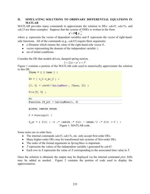
Consider the DE that models driven, damped spring motion.
2
x 2 x x
F
2 x
Figure 1 contains a portion of the MATLAB code used to numerically approximate the solution
to this DE.
Figure 1: MATLAB code.
Some notes are in order here.
The internal commands ode45, ode15s, etc. only accept first-order DEs.
Many higher-order DEs may be transformed into systems of first-order DEs.
The order of the formal arguments in SpringMass is important.
T represents the values of the independent variable t generated by ode45.
Each row in X represents the value of X corresponding to the associated time value in T.
Once the solution is obtained, the output may be displayed via the internal command plot; frills
may be added as needed. Figure 2 contains the portion of code used to display the
approximation.
235