Projects with applications of differential equations - Mathematics ...
Projects with applications of differential equations - Mathematics ...
Projects with applications of differential equations - Mathematics ...

Create successful ePaper yourself
Turn your PDF publications into a flip-book with our unique Google optimized e-Paper software.
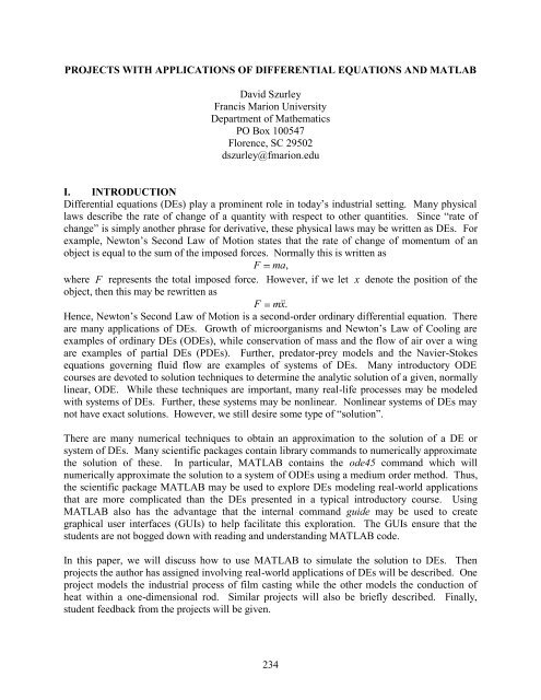
PROJECTS WITH APPLICATIONS OF DIFFERENTIAL EQUATIONS AND MATLAB<br />
David Szurley<br />
Francis Marion University<br />
Department <strong>of</strong> <strong>Mathematics</strong><br />
PO Box 100547<br />
Florence, SC 29502<br />
dszurley@fmarion.edu<br />
I. INTRODUCTION<br />
Differential <strong>equations</strong> (DEs) play a prominent role in today’s industrial setting. Many physical<br />
laws describe the rate <strong>of</strong> change <strong>of</strong> a quantity <strong>with</strong> respect to other quantities. Since “rate <strong>of</strong><br />
change” is simply another phrase for derivative, these physical laws may be written as DEs. For<br />
example, Newton’s Second Law <strong>of</strong> Motion states that the rate <strong>of</strong> change <strong>of</strong> momentum <strong>of</strong> an<br />
object is equal to the sum <strong>of</strong> the imposed forces. Normally this is written as<br />
F ma m ,<br />
where F represents the total imposed force. However, if we let x denote the position <strong>of</strong> the<br />
object, then this may be rewritten as<br />
F m x<br />
.<br />
Hence, Newton’s Second Law <strong>of</strong> Motion is a second-order ordinary <strong>differential</strong> equation. There<br />
are many <strong>applications</strong> <strong>of</strong> DEs. Growth <strong>of</strong> microorganisms and Newton’s Law <strong>of</strong> Cooling are<br />
examples <strong>of</strong> ordinary DEs (ODEs), while conservation <strong>of</strong> mass and the flow <strong>of</strong> air over a wing<br />
are examples <strong>of</strong> partial DEs (PDEs). Further, predator-prey models and the Navier-Stokes<br />
<strong>equations</strong> governing fluid flow are examples <strong>of</strong> systems <strong>of</strong> DEs. Many introductory ODE<br />
courses are devoted to solution techniques to determine the analytic solution <strong>of</strong> a given, normally<br />
linear, ODE. While these techniques are important, many real-life processes may be modeled<br />
<strong>with</strong> systems <strong>of</strong> DEs. Further, these systems may be nonlinear. Nonlinear systems <strong>of</strong> DEs may<br />
not have exact solutions. However, we still desire some type <strong>of</strong> “solution”.<br />
There are many numerical techniques to obtain an approximation to the solution <strong>of</strong> a DE or<br />
system <strong>of</strong> DEs. Many scientific packages contain library commands to numerically approximate<br />
the solution <strong>of</strong> these. In particular, MATLAB contains the ode45 command which will<br />
numerically approximate the solution to a system <strong>of</strong> ODEs using a medium order method. Thus,<br />
the scientific package MATLAB may be used to explore DEs modeling real-world <strong>applications</strong><br />
that are more complicated than the DEs presented in a typical introductory course. Using<br />
MATLAB also has the advantage that the internal command guide may be used to create<br />
graphical user interfaces (GUIs) to help facilitate this exploration. The GUIs ensure that the<br />
students are not bogged down <strong>with</strong> reading and understanding MATLAB code.<br />
In this paper, we will discuss how to use MATLAB to simulate the solution to DEs. Then<br />
projects the author has assigned involving real-world <strong>applications</strong> <strong>of</strong> DEs will be described. One<br />
project models the industrial process <strong>of</strong> film casting while the other models the conduction <strong>of</strong><br />
heat <strong>with</strong>in a one-dimensional rod. Similar projects will also be briefly described. Finally,<br />
student feedback from the projects will be given.<br />
234
II. SIMULATING SOLUTIONS TO ORDINARY DIFFERENTIAL EQUATIONS IN<br />
MATLAB<br />
MATLAB provides many commands to approximate the solution to DEs: ode45, ode15s, and<br />
ode23 are three examples. Suppose that the system <strong>of</strong> ODEs is written in the form<br />
y' f t,<br />
y ,<br />
where y represents the vector <strong>of</strong> dependent variables and f represents the vector <strong>of</strong> right-handside<br />
functions. All <strong>of</strong> the commands (e.g., ode45) require three arguments:<br />
a filename which returns the value <strong>of</strong> the right-hand-side vector f ,<br />
vector representing the domain <strong>of</strong> the independent variable t ,<br />
set <strong>of</strong> initial conditions.<br />
Consider the DE that models driven, damped spring motion.<br />
2<br />
x 2 x x<br />
F<br />
2 x<br />
Figure 1 contains a portion <strong>of</strong> the MATLAB code used to numerically approximate the solution<br />
to this DE.<br />
Figure 1: MATLAB code.<br />
Some notes are in order here.<br />
The internal commands ode45, ode15s, etc. only accept first-order DEs.<br />
Many higher-order DEs may be transformed into systems <strong>of</strong> first-order DEs.<br />
The order <strong>of</strong> the formal arguments in SpringMass is important.<br />
T represents the values <strong>of</strong> the independent variable t generated by ode45.<br />
Each row in X represents the value <strong>of</strong> X corresponding to the associated time value in T.<br />
Once the solution is obtained, the output may be displayed via the internal command plot; frills<br />
may be added as needed. Figure 2 contains the portion <strong>of</strong> code used to display the<br />
approximation.<br />
235
Figure 2: MATLAB code used to produce the display <strong>of</strong> the approximation.<br />
The natural next step is to provide students <strong>with</strong> this code and ask questions. For example, one<br />
could ask students what is the effect <strong>of</strong> changing the damping coefficient. In order for the<br />
students to answer this question, they are required to determine the line(s) in the code where the<br />
damping coefficient is defined, appropriately change those, and rerun the code. This process<br />
demonstrates a drawback to using this approach: it is difficult for the students to read and<br />
understand code.<br />
One solution to this problem is the use <strong>of</strong> GUIs. They provide a means <strong>of</strong> introducing students<br />
to scientific packages <strong>with</strong>out entirely involving the students <strong>with</strong>in the code. Instead <strong>of</strong><br />
expecting students to modify code, they may simply edit text and click a button. The required<br />
calculations are then accomplished for the students <strong>with</strong>out being visible. The MATLAB<br />
internal command guide is the GUI development interface. It enables simplified arrangement<br />
and sizing <strong>of</strong> GUI components as well as auto-generation <strong>of</strong> code for these components.<br />
Examples <strong>of</strong> GUI components would be push buttons, axes, sliders, pop-up menus, among<br />
others. Figure 3 displays an example GUI for the spring-mass system.<br />
Figure 3: Example GUI for the spring-mass system.<br />
236
The students may change the quantities by simply typing the new value in the edit text boxes and<br />
rerun the code by pressing the push button. With this GUI, it is easier for students to answer<br />
questions related to changing system parameters. Now the students may explore the particular<br />
model by being provided <strong>with</strong> the GUI and some auxiliary files.<br />
III. PROJECTS<br />
Students enrolled in an introductory ordinary <strong>differential</strong> <strong>equations</strong> course were grouped up and<br />
given different projects. Each project involved an industrial process that may be modeled by<br />
DEs. The students were asked to understand the process, why it is useful, how the process is<br />
modeled, and to present their results at a conference. There were four main thrusts <strong>of</strong> the<br />
projects.<br />
Expose students to a real-world process<br />
Expose students to a scientific s<strong>of</strong>tware package (MATLAB)<br />
Demonstrate the need for numerical schemes<br />
Gain experience in public speaking via presentation <strong>of</strong> their results<br />
IV. FILM CASTING<br />
Today’s society has in great abundance products that are made from polymers: clothing made<br />
from synthetic fibers, plastic bags, food wrap, and disposable diapers are among the most<br />
common examples. It has become imperative for today’s manufacturers to understand the<br />
processes used to make these products as fully as possible. The processes involve complex fluid<br />
flow <strong>of</strong> a molten polymer, governed by systems <strong>of</strong> DEs.<br />
Film casting is an industrial process in which fluid (molten polymer) is extruded from a<br />
rectangular die <strong>of</strong> thickness e 0 and length l 0 , at a temperature T 0 , and a velocity u 0 . Please see<br />
[1], [3], [6], [9] – [12], and [13] for a detailed description <strong>of</strong> the process. The fluid is then<br />
stretched in the air due to the constant pulling force F <strong>of</strong> the chill roll, located at a distance <strong>of</strong> L<br />
from the die. The film is then cooled on this chill roll to solidify the fluid. The film casting<br />
process is shown in Figure 4.<br />
Figure 4: Schematic <strong>of</strong> the film casting process.<br />
237
The five dependent variables <strong>of</strong> the flow are length l , velocity u , pulling force F , temperature<br />
T , and thickness e . Under certain assumptions, the <strong>equations</strong> governing this process may be<br />
dl<br />
dx<br />
du<br />
dx<br />
dT<br />
dx<br />
12<br />
1<br />
24<br />
given as follows.<br />
u<br />
l<br />
2<br />
h T<br />
C<br />
ue<br />
p<br />
2<br />
F<br />
8<br />
A<br />
36<br />
2l<br />
2<br />
2<br />
u<br />
F<br />
A<br />
T<br />
2<br />
2<br />
F<br />
A<br />
2<br />
T<br />
l<br />
4<br />
2<br />
T<br />
dl e<br />
dx l<br />
This is a system <strong>of</strong> five first order nonlinear ODEs. Further, while the initial conditions for<br />
length, velocity, temperature, and thickness are simply those at the die exit, the initial pulling<br />
force F 0 is not known a priori. The numerical technique <strong>of</strong> shooting is used to determine the<br />
value <strong>of</strong> F 0 . As opposed to attempting to solve this system analytically, it would be better to<br />
numerically approximate the solution using a numerical package (e.g., ode45).<br />
Code was written that will numerically simulate the solution to these <strong>equations</strong> given a set <strong>of</strong><br />
parameters. Moreover, a GUI was designed so that students were required to only edit the<br />
parameters. Figure 5 displays the GUI provided to the students as well as a typical solution<br />
pr<strong>of</strong>ile. Students were asked to change the set <strong>of</strong> parameters and to determine the effect the<br />
change had on the solution.<br />
dF<br />
dx<br />
de<br />
dx<br />
AAu<br />
d<br />
dx<br />
du<br />
dx<br />
Figure 5: GUI and typical solution pr<strong>of</strong>ile for the film casting problem.<br />
4<br />
238<br />
e<br />
AAg<br />
du<br />
dx<br />
e<br />
u
V. HEAT CONDUCTION IN A ONE-DIMENSIONAL ROD<br />
The manner in which heat is transferred <strong>with</strong>in a one-dimensional rod may be modeled <strong>with</strong> a<br />
PDE. We assume an initial temperature distribution and desire to know how heat is conducted<br />
<strong>with</strong>in the rod as time evolves. The PDE that models heat conduction may be given by<br />
u<br />
t<br />
k<br />
2<br />
u<br />
, 2<br />
x<br />
where k is the thermal diffusivity (see [8]). We assume that the initial temperature distribution<br />
is prescribed and that the temperature at the ends <strong>of</strong> the rod ( x 0 and x L ) are given. Hence<br />
the boundary and initial conditions are<br />
u(<br />
0,<br />
t)<br />
u(<br />
L,<br />
t)<br />
u(<br />
x,<br />
0)<br />
0 0,<br />
0 0,<br />
f ( x).<br />
Since this is a PDE, the suite <strong>of</strong> ODE solvers in MATLAB are inappropriate. Hence, we choose<br />
to numerically approximate the solution to this PDE via the finite difference method (FDM). See<br />
[8] for a rough description <strong>of</strong> the FDM. The FDM first takes the continuous domain in the xt -<br />
plane and replaces it <strong>with</strong> a discrete mesh, as shown in Figure 6.<br />
Figure 6: Example <strong>of</strong> a FDM mesh.<br />
Next, the partial derivatives in the PDE itself are replaced <strong>with</strong> approximately equivalent<br />
( m)<br />
difference quotients. If we let u j u ( x j , tm<br />
) , choose to approximate<br />
u <strong>with</strong> a forward<br />
t<br />
difference and<br />
equation.<br />
2<br />
u<br />
<strong>with</strong> a centered difference, we obtain the following finite difference<br />
2<br />
t<br />
( m<br />
u j<br />
1<br />
)<br />
( m)<br />
u<br />
j<br />
k<br />
t<br />
2<br />
x<br />
( m)<br />
)<br />
u j 1<br />
( m)<br />
2 2u<br />
j<br />
( m )<br />
u j 1<br />
239
Code was written to solve the finite difference equation and display the results. Once the code<br />
was working properly, a GUI was designed to allow students to numerically approximate the<br />
solution for a given parameter set. Figure 7 shows the GUI as well as a solution pr<strong>of</strong>ile for a<br />
parameter set.<br />
Figure 7: GUI and solution pr<strong>of</strong>ile for heat conduction in a one-dimensional rod.<br />
Students were asked to change the initial condition and the thermal diffusivity to determine the<br />
effect on the solution pr<strong>of</strong>ile.<br />
VI. FIBER SPINNING PROJECTS<br />
Two projects involved the industrial process <strong>of</strong> fiber spinning (see [2], [4], [5], [7], and [14]).. In<br />
this process, an axisymmetric stream <strong>of</strong> polymer melt is extruded from a spinneret containing<br />
thousands <strong>of</strong> capillaries. The spinneret may be thought <strong>of</strong> roughly as a shower head. The<br />
polymer melt is then drawn continuously by the take-up rolls. Along the length <strong>of</strong> the stream,<br />
there is a region where cooling air is applied. This process is illustrated in Figure 8.<br />
240
Figure 8: Schematic <strong>of</strong> the fiber spinning process.<br />
Depending upon the processing parameters, the polymer may enter a semi-crystalline phase<br />
where the structure <strong>of</strong> the molecules <strong>of</strong> the polymer cannot change. One project explored fiber<br />
spinning excluding the semi-crystalline phase, while the other project considered both phases.<br />
Both processes are governed by systems <strong>of</strong> nonlinear ordinary <strong>differential</strong> <strong>equations</strong>.<br />
VII. WAVE PROPAGATION PROJECT<br />
The final project explored the propagation <strong>of</strong> waves on a taut string (see [8]). This process is<br />
governed by the following PDE.<br />
2<br />
2<br />
u 2 u<br />
c<br />
2<br />
2<br />
t<br />
x<br />
Here c represents the propagation speed <strong>of</strong> the wave. The following boundary and initial<br />
conditions are enforced.<br />
u(<br />
0,<br />
t)<br />
u(<br />
L,<br />
t)<br />
u(<br />
x,<br />
0)<br />
0<br />
0<br />
f<br />
( x)<br />
u<br />
( x,<br />
0)<br />
g<br />
( x)<br />
t<br />
Figure 9 displays the GUI provided to the students as well as an example solution pr<strong>of</strong>ile.<br />
\<br />
241
Figure 9: GUI and solution pr<strong>of</strong>ile for wave propagation on a taut string.<br />
Students were asked to change the initial displacement <strong>of</strong> the string and the propagation speed to<br />
determine the effect on the solution pr<strong>of</strong>ile.<br />
VIII. STUDENT FEEDBACK<br />
Student response from these projects differed between the objectives <strong>of</strong> the projects. Student<br />
responses were generally positive about exploring real-world <strong>applications</strong> <strong>of</strong> DEs and the<br />
experience gained in public speaking. However, the responses were generally mediocre for the<br />
numerical schemes and the exposure to MATLAB. Many students were surprised that DEs<br />
modeling real-world <strong>applications</strong> could not be solved analytically. Overall, the students gave the<br />
projects positive reviews and considered them a success.<br />
REFERENCES<br />
[1] Acierno, D., L. Di Maio, C. Ammirati, “Film Casting <strong>of</strong> Polyethylene Terephthalate:<br />
Experiments and Model Comparisons,” Polymer Engineering and Science, Vol. 40, pp. 108-<br />
117, 2000.<br />
[2] Advani, S., C. Tucker III, “The Use <strong>of</strong> Tensors to Describe and Predict Fiber Orientation In<br />
Short Fiber Composites,” Journal <strong>of</strong> Rheology, Vol. 31, pp. 751-784, 1987.<br />
[3] Baird, D., D. Collais, Polymer Processing, John Wiley and Sons, New York, 1998.<br />
[4] Denn, M., Process Modeling, Longman Inc., New York, 1986.<br />
[5] Doufas, A., A, McHugh, C. Miller, “Simulation <strong>of</strong> Melt Spinning Including Flow-Induced<br />
Crystallization Part I: Model Development and Predictions,” Journal <strong>of</strong> Non-Newtonian<br />
Fluid Mechanics, Vol. 92, pp. 27-66, 2000.<br />
[6] Eisele, P., R. Killpack, “Propene,” Ullman’s Encyclopedia <strong>of</strong> Industrial Chemistry, 1993 ed.<br />
[7] Fisher, R., M. Denn, “Mechanics <strong>of</strong> Nonisothermal Polymer Melt Spinning,” American<br />
Institute <strong>of</strong> Chemical Engineers Journal, Vol. 23, No. 1, pp. 23-28.<br />
[8] Haberman, R., Elementary Applied Partial Differential Equations, Prentice Hall, New Jersey,<br />
1987.<br />
[9] Lide, D., ed. CRC Handbook <strong>of</strong> Chemistry and Physics, CRC Press, New York, 2001.<br />
[10] Mark, J., ed. Physical Properties <strong>of</strong> Polymers Handbook, AIP Press New York 1996.<br />
242
[11] Smith, S., D. Stolle, “Nonisothermal Two-Dimensional Film Casting <strong>of</strong> a Viscous<br />
Polymer,” Polymer Engineering and Science, Vol. 40, pp. 1870-1877, 2000.<br />
[12] Vargaftik, N., Tables on the Thermophysical Properties <strong>of</strong> Liquids and Gases, John<br />
Wiley and Sons, New York, 1975.<br />
[13] Ziabicki, A., Fundamentals <strong>of</strong> Fibre Formation, John Wiley and Sons, New York, 1976.<br />
[14] Ziabicki, A., L. Jarecki, A. Waiak, “Dynamic Modelling <strong>of</strong> Melt Spinning,”<br />
Computational and Theoretical Polymer Science, Vol. 8, pp. 143-157, 1998.<br />
243