Projects with applications of differential equations - Mathematics ...

V. HEAT CONDUCTION IN A ONE-DIMENSIONAL ROD
The manner in which heat is transferred within a one-dimensional rod may be modeled with a
PDE. We assume an initial temperature distribution and desire to know how heat is conducted
within the rod as time evolves. The PDE that models heat conduction may be given by
u
t
k
2
u
, 2
x
where k is the thermal diffusivity (see [8]). We assume that the initial temperature distribution
is prescribed and that the temperature at the ends of the rod ( x 0 and x L ) are given. Hence
the boundary and initial conditions are
u(
0,
t)
u(
L,
t)
u(
x,
0)
0 0,
0 0,
f ( x).
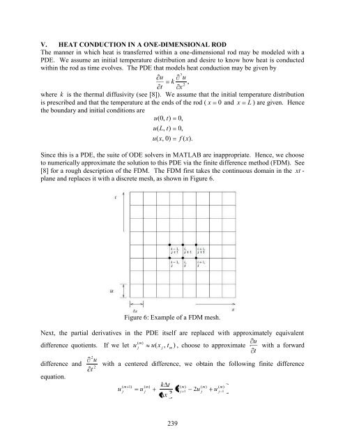
Since this is a PDE, the suite of ODE solvers in MATLAB are inappropriate. Hence, we choose
to numerically approximate the solution to this PDE via the finite difference method (FDM). See
[8] for a rough description of the FDM. The FDM first takes the continuous domain in the xt -
plane and replaces it with a discrete mesh, as shown in Figure 6.
Figure 6: Example of a FDM mesh.
Next, the partial derivatives in the PDE itself are replaced with approximately equivalent
( m)
difference quotients. If we let u j u ( x j , tm
) , choose to approximate
u with a forward
t
difference and
equation.
2
u
with a centered difference, we obtain the following finite difference
2
t
( m
u j
1
)
( m)
u
j
k
t
2
x
( m)
)
u j 1
( m)
2 2u
j
( m )
u j 1
239