SIAR V4 (Stable Isotope Analysis in R) An Ecologist's Guide

SIAR V4
(Stable Isotope Analysis in R)
An Ecologist’s Guide
Richard Inger, Andrew Jackson, Andrew Parnell & Stuart Bearhop
density
0 5 10 15
0.0 0.2 0.4 0.6 0.8 1.0
0.0 0.2 0.4 0.6 0.8 1.0
ZosteraG1
-0.14
-0.41
0.0 0.2 0.4 0.6 0.8 1.0 0.0 0.2 0.4 0.6 0.8 1.0
GrassG1
-0.53 -0.40
0.0 0.2 0.4 0.6 0.8 1.0
Proportion densities for group 1
0.0 0.2 0.4 0.6 0.8 1.0
0.25
proportion
Matrix plot of proportions for group 1
U.lactucaG1
-0.50
0.0 0.2 0.4 0.6 0.8 1.0
Zostera
Grass
U.lactuca
Enteromorpha
EnteromorphaG1
0.0 0.2 0.4 0.6 0.8 1.0
0.0 0.2 0.4 0.6 0.8 1.0
d15N
5 10 15 20
Proportion
0.0 0.2 0.4 0.6 0.8 1.0
Zostera
Grass
U.lactuca
Enteromorpha
Group 1
Group 2
Group 3
Group 4
Group 5
Group 6
Group 7
Group 8
SIAR data
-30 -25 -20 -15 -10 -5
d13C
Proportions by source: Zostera
1 2 3 4 5 6 7 8
Group
1

Contents Page
1. Introduction 3
2. Installation of R 3
3. Installation of SIAR 3
4. Working with SIAR 5
4.1. Menu System or Scripts 5
4.2. Data Structure 5
4.3. Multiple Data Points 6
4.3.1. Structure of the Input Files 6
4.3.2. Data Input 7
4.3.3. Running the Model 7
4.3.4. Plotting the Results 8
4.3.4.1. Plotting the Raw Data 8
4.3.4.2. Diagnostic matrix plot 8
4.3.4.3. Histogram Plot 9
4.3.4.4. Boxplot of Proportions by Group 10
4.3.4.5. Boxplot of Proportions by Source 11
4.3.5. Accessing the Raw Output Data 11
4.4. Single Data Points 12
4.5. Concentration Dependence Models 12
4.6 Incorporating Prior Information into Models 12
4.7. Troubleshooting 13
5. Recommended Reading 14
2

1. Introduction
SIAR is a package designed to solve mixing models for stable isotopic data within a Bayesian
framework. This guide is designed to get researchers up and running with the package as
quickly as possible. No expertise is required in the use of R.
We assume that you have a sound working knowledge of stable isotopic mixing models, and
the assumptions and potential pitfalls associated with these models. Failure to take account of
these assumptions could lead to erroneous results. A list of required reading is presented in
Appendix A of this guide. We strongly recommend that all users unfamiliar with isotopic
mixing models read these papers.
SIAR will always try to fit a model even if the data are nonsensical.
Further information on the SIAR package is available from:
http://cran.r-­‐project.org/web/packages/siar/siar.pdf
The examples shown here are based on the dataset presented in Inger et al. 2006. A subset of
this dataset is provided with the SIAR package
2. Installation of R
R is available for virtually all operating systems, including Microsoft Windows, Mac OS, Linux
and a wide variety of UNIX platforms. R can be downloaded from http://www.r-­‐project.org/
and installed by following the instructions on the R website.
From the home page click the download R link.
Then select the CRAN mirror nearest to you.
Then select your operating system.
Windows -­‐ select the base ‘Binaries for base distribution’ option. Then click on the Download
R link. An executable file will then be downloaded. Double click on this to run the installation
program and follow the on screen instructions.
Max OS -­‐ select the R-2.11.0.pkg link, then click on the downloaded package, which will run
the installer, then follow the instructions.
Linux / UNIX – if your running either of these we assume you can do this!
3. Installation of the SIAR package
Windows
Start R and select packages from the menu, then install package(s)… Then select your nearest
CRAN mirror from the list, and finally scroll down to find ‘siar’ on the list and click on it. You
will then see lots of activity on the screen as the SIAR package and the other packages it uses
are downloaded. The final line should then read:
package 'siar' successfully unpacked and MD5 sums checked
You then need to load the package. Type:
3

library(siar)
This will load the package and all the associated packages. You’ll need to do this every time
you start R, or you can make R install packages automatically on start up (see R help pages).
Alternatively, you can install the SIAR package by typing command;
install.packages(‘siar’)
MacOS
Start R and select ‘Packages and Data’ then package installer at which point a new window
opens. Type ‘siar’ into the search box, and click on ‘get list’, then ensure that the ‘install
dependencies’ box is ticked, and click on siar, then click ‘install selected’. You’ll then see lots
of on screen activity as the packages are downloaded. The final message should begin with:
The downloaded packages are in /var/folders . . . .
You then need to load the package. Type:
library(siar)
This will load the package and all the associated packages. You’ll need to do this every time
you start R, or you can make R install packages automatically on start up (see R help pages).
4

4. Working with SIAR
Before getting started there are a couple of points to consider.
4.1. Menu System or Scripts
There are two ways to run the SIAR package. Firstly via the built in menu system, or secondly,
via scripts. We strongly recommend using the latter option as the menu system was only ever
designed as an introduction to the package. Accessing the package by running scripts offers a
much greater level of flexibility and allows those with some coding experience to develop
scripts to run multiple analyses or carry out post-­‐hoc tests on the outputs from SIAR. Scripts
can be written using the built in script editor or via external editors. In our experience the
built in Mac editor is quite good, although the windows version is somewhat limited, and we
would recommend using Tinn-­‐R, which is available as a free download. Once your script has
been written, save it and then either send it to R from the script editor, or call it from R using
the ‘source’ command.
4.2. Data Structure.
Are you interested in determining the source proportions based on single or multiple data
points? In most analyses you will most likely require some sort of grouping variable. The
different groups could represent for example:
• Different demographic groups.
• Different sampling periods.
• Different sampling locations.
• Different samples from the same individual.
In the case of the example data that comes with the SIAR package the grouping variable is the
month of capture/sampling. See Inger et al. 2006 for further details
This is the default mode for SIAR. Currently up to 30 groups can be used in a single analysis.
You must include more than one observation per group, and really there should be at least 3
but preferably 5 or more per group in order to be able to estimate intra-­‐group variances.
If you only have one data point for each individual / observational group then you should use
the ‘siarsolo’ command. This works in exactly the same way as the default, but does not
include the residual error term (See Parnell et al. 2010 for further details).
5

4.3. Multiple Data points
4.3.1. Structure of the input files.
SIAR requires 3 input files. All files should be tab separated .txt files. These can be generated
in MS Excel or in any basic text editor.
1) The consumer data file contains the stable isotopic data for you consumers and should
consist of columns, firstly the grouping variable, secondly the data for isotope 1, thirdly the
data for isotope 2. More or fewer isotopes can be used.
Example consumer data file:
Code d15N d13C
1 9.1 -­‐10.48
1 10.16 -­‐11.78
1 8.78 -­‐11.41
2 9.42 -­‐10.47
2 9.26 -­‐10.58
2) The sources data file. This file contains the data on the different sources contributing to the
consumer. The data can be input as mean and standard deviation for each source. N.B. the
order of occurrence of each isotope must match that in the consumer data file.
Example source data file:
Source Meand15N SDd15N Meand13C SDd13C
Zostera 6.49 1.21 -­‐11.17 1.21
Grass 4.43 0.64 -­‐30.88 0.64
U.lactuca 11.19 1.96 -­‐11.17 1.96
Enteromorpha 9.82 1.17 -­‐14.06 1.17
3) The Trophic Enrichment Factor (TEF) data file. This contains the TEFs as mean and
standard deviation for each source. TEFs can also be refereed to as fractionation /
discrimination factors within the literature. Again, the order of occurrence of each isotope
must match that in the consumer data file.
Example TEF data file:
Source Meand15N SDd15N Meand13C SDd13C
Zostera 3.54 0.74 1.63 0.63
Grass 3.54 0.74 1.63 0.63
U.lactuca 3.54 0.74 1.63 0.63
Enteromorpha 3.54 0.74 1.63 0.63
Note Different TEFs can be applied to different sources.
There is an additional file that can also be incorporated into the model with the elemental
concentration values. See Section 4.5.
6

Note Ensure that there are no spaces in the header columns(as R will interpret the white
spaces as a new entry and it will think there are more columns than you do), and that the
order of the isotopes are the same for all the files.
4.3.2. Data Input
Once your data is in the correct format you’ll need to read it into R. So, the first few lines of
you script should look something like this:
data

4.3.4. Plotting the results.
There are a number of plotting options available within the SIAR package.
4.3.4.1. Plotting the raw data
Firstly lets have a look at the raw isotopic data. This can be done using:
siarplotdata(model1)
This will produce a biplot with the isotope that is in the first column on the x-­‐axis, and the
isotope in the second column on the y-­‐axis. Once the command is executed a crosshair will
appear in the cursor position, click on the plot to position the legend.
This will produce something like this:
Note The TEFs are added to the sources rather than subtracted from the consumers. This is to
allow different TEFs to be assigned to different sources.
4.3.4.2. Diagnostic Matrix Plot
d15N
5 10 15 20
Zostera
Grass
U.lactuca
Enteromorpha
Group 1
Group 2
Group 3
Group 4
Group 5
Group 6
Group 7
Group 8
SIAR data
-30 -25 -20 -15 -10 -5
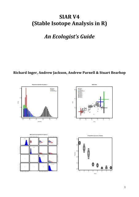
Next, you can produce a matrix plot, which shows histograms for the estimate of each
proportion on the main diagonal. The contour plots in the upper triangle shows how pairs (by
rows and columns) of posterior distributions are correlated (if at all) and the actual
correlation coefficient is given in the lower triangle. These correlation plots and statistics are
generated by pairing simulated values of the dietary proportions drawn by each iteration of
the MCMC process (so for each draw they must sum to one). This is a useful diagnostic tool as
it will identify when the model is performing well, indicated by low correlations between
sources, or when the model is struggling to differentiate between sources, as indicated by
higher correlations. For instance, if two sources are very close together, then likely solutions
could involve one or other of the sources but not both at the same time. In such a scenario,
these two sources would be expected to show negative correlation in their posterior
distributions. This is evident in the isotope biplot for Enteromorpha and U. lactuca, which
then show negative correlation in the contour plot of their joint posterior distribution for
Group 1. Positive correlations are also possible, where a solution that involves one source,
may necessisarily require another source in some proportion so as to balance each other out
d13C
8

and provide a sensible solution to the mixing problem. See section 4.3.5. for details on how to
access the full set of posterior draws should you wish to perform additional analyses.
To produce the plot:
siarmatrixplot(model1)
Once the command is executed you will be prompted to enter a group number, after which the
plot will be created.
4.3.4.3. Histogram Plot
SIAR can produce histograms of the distribution of possible solutions for all sources in the
model. These plots will be familiar to anyone’s who’s used ISOSOURCE. The difference here is
that SIAR produces true probability density functions. To produce histograms:
siarhistograms(model1)
You will then be prompted to select the group you which to plot, and also if you require all the
sources separately or on one plot. If you select the latter option you will get a plot like this:
density
0 5 10 15
0.0 0.2 0.4 0.6 0.8 1.0
0.0 0.2 0.4 0.6 0.8 1.0
ZosteraG1
-0.14
-0.41
0.0 0.2 0.4 0.6 0.8 1.0 0.0 0.2 0.4 0.6 0.8 1.0
GrassG1
-0.53 -0.40
0.0 0.2 0.4 0.6 0.8 1.0
Matrix plot of proportions for group 1
0.25
U.lactucaG1
-0.50
0.0 0.2 0.4 0.6 0.8 1.0
Proportion densities for group 1
EnteromorphaG1
0.0 0.2 0.4 0.6 0.8 1.0
proportion
Zostera
Grass
U.lactuca
Enteromorpha
0.0 0.2 0.4 0.6 0.8 1.0
0.0 0.2 0.4 0.6 0.8 1.0
9

4.3.4.4. Boxplot of Proportions by Group
SIAR can also produce boxplots of the proportions of different sources. To compare the
proportions of each source for a group:
siarproportionbygroupplot(model1)
At which point you will be asked to pick which source you want to plot, and SIAR will then
produce something like this:
There are additional arguments that can be included in this command.
prn If prn=TRUE then the values for the probability densities are returned to the
command line.
grp Specifies the group to be plotted
probs Defines the credibility intervals to be plotted. The default is 95, 75 and 25%.
Other values should be added in the format c(10, 50, 90).
type Defines the type of plot. The Default is boxes, type=”lines” produces a plot using
different thickness lines.
clr Sets the colour of the boxes. Default is greyscale.
scl Sets the width of the boxes or lines. Default is 1.
xspc Sets the amount of blank space before the first and after the last box / line.
leg Allows a legend to be added to the plot if leg=TRUE. Only works with line plots
So:
Proportion
0.0 0.2 0.4 0.6 0.8 1.0
Proportions by group: 1
Zostera Grass U.lactuca Enteromorpha
siarproportionbysourceplot(model1, prn=TRUE,grp=1,probs=c(5,25,75,95))
Source
Will return the probability densities to the command line, produce a plot for group 1, and plot
the 5, 25, 75 and 95% credibility internals.
10

4.3.4.5. Boxplot of Proportions by Source
SIAR also allows you to plot the proportions of each group by source, allowing a comparison
of sources for different groups:
siarproportionbygroupplot(model1)
Which will ask you for which group you want to plot. SIAR will then produce a plot like this:
The additional arguments are the same as for the siarproportionbysourceplot command.
4.3.5. Accessing the Raw Output Data.
The raw output from the model is stored in a matrix called output, which is in the R object
created earlier called model1. So we can create a new matrix with this data in:
out

Obtaining extra data from the raw data is easy. For example if you want the mean value for
group1, source 1 enter:
mean(out[,1])
Square brackets are used to define subscripts in R, so [1,1] would return the values in the first
row and first column. [,1] selects all of the first column.
4.4. Single Data points
If you only have single data points (or sets of data points for multiple isotopes) then almost
everything is the same as for the multiple data points approach.
You data should be set up such that each data point is coded 1 to n:
Code d15N d13C
1 9.1 -­‐10.48
2 10.16 -­‐11.78
3 8.78 -­‐11.41
4 9.42 -­‐10.47
5 9.26 -­‐10.58
Then instead of using the siarmcmcdirichletv4 command use the siarsolomcmcv4 command:
model1

prior distribution in SIAR, by expressing the estimated mean of each proportion and a
standard deviation for the first given proportion. This restriction (giving only one standard
deviation) is required because of the Dirichlet prior distribution used by SIAR to model the
dietary proportions. The function siarelicit can be called after a standard run of SIAR (ie with
a non-­‐informative prior). The command:
siarelicit(model1)
will bring up a set of instructions for entering prior data. Suppose we know that the 4 dietary
proportion means should be in the range of 0.7, 0.15, 0.08, 0.07 (note that they must sum to
1), and that the first should be in the range from 0.65 to 0.75. (ie 95% CI width of 0.05), and
therefore standard deviation width of approximately 0.025. We can then enter these
proportions and standard deviations as instructed. siarelicit will return prior values for the
new run. Here, these are: 234.5, 50.25, 26.8, 23.45. We use these in a new run of SIAR:
model2

5. Recommended Reading
Phillips, D.L. (2001) Mixing models in analyses of diet using multiple stable isotopes: a
critique. Oecologia, 127, 166-­‐170
Phillips, D.L. & Gregg, J.W. (2001) Uncertainty in source partitioning using stable isotopes.
Oecologia, 127, 171-­‐179
Phillips ,D.L. & Koch, P.L. (2002) Incorporating concentration dependence in stable isotope
mixing models. Oecologia, 130, 114-­‐125
Phillips, D.L. & Gregg, J.W. (2003) Source partitioning using stable isotopes: coping with too
many sources. Oecologia, 136, 261-­‐269
Phillips, D.L., Newsome, S.D. & Gregg, J.W. (2005) Combining Sources in stable isotope mixing
models: alternative methods. Oecologia, 144, 520-­‐527
Moore, J.W. & Semmens, B.X. (2008) Incorporating uncertainty and prior information into
stable isotope mixing models. Ecology Letters, 11, 470-­‐480
Jackson, A, Inger, R., Bearhop, S. & Parnell, A. (2009) Erroneous behaviour of MixSIR, a
recently published Bayesian isotope mixing model: a discussion of Moore & Semmens,
Ecology Letters, 2008. Ecology Letters, 12, E1–E5.
Parnell, A., Inger, R., Bearhop, S. & Jackson, A.L. (2010) Source partitioning using stable
isotopes: coping with too much variation. PlosOne, 5(3): e9672.
Inger, R., Ruxton, G.D., Newton, J., Colhoun, K., Robinson, J.A., Jackson, A.L., & Bearhop, S.
(2006) Temporal and intrapopulation variation in prey choice of wintering geese
determined by stable isotope analysis. Journal of Animal Ecology, 75, 1190-­‐1200.
14