Xilinx Exemplar/ModelSim Tutorial for CPLDs

Exemplar/ModelSim Tutorial for CPLDs 

Design Description 

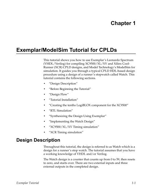
Chapter 1 

This tutorial shows you how to use Exemplar’s Leonardo Spectrum 

(VHDL/Verilog) for compiling XC9500/XL/XV and Xilinx Cool- 

Runner (XCR) CPLD designs, and Model Technology’s ModelSim for 

simulation. It guides you through a typical CPLD HDL-based design 

procedure using a design of a runner’s stopwatch called Watch. This 

tutorial contains the following sections. 

• “Design Description” 

• “Before Beginning the Tutorial” 

• “Design Flow” 

• “Tutorial Installation” 

• “Creating the tenths LogiBLOX component for the XC9500” 

• “RTL Simulation” 

• “Synthesizing the Design Using Exemplar” 

• “Implementing the Watch Design” 

• “XC9500/XL/XV Timing simulation” 

• “XCR Timing simulation” 

Throughout this tutorial, the design is referred to as Watch which is a 

design for a runner’s stop watch. The tutorial assumes that you have 

a working knowledge of VHDL and/or Verilog. 

The Watch design is a counter that counts up from 0 to 59, then resets 

to zero, and starts over. There are two external inputs and three 

external outputs in the completed design. 

Exemplar Tutorial 1-1

Exemplar Tutorial 

There is a companion Watch tutorial for Xilinx FPGAs, which have an 

on chip oscillator. Xilinx CPLDs do not have an on chip oscillator, and 

most of the differences in the tutorials are due to the use of an 

external system clock for the CPLD. 

The Watch design inputs, outputs, and modules are summarized 

below. 

Inputs 

• STRTSTOP—The start/stop button of the stopwatch. This is an 

active-low signal that must be depressed then released to start or 

stop the counting. 

• RESET—Forces the signals TENSOUT and ONESOUT to be “00” 

after the stopwatch has been stopped. 

• CLK — Externally supplied system clock. A 36 KHz clock is used 

on XCR demo board. 

Outputs 

• TENSOUT[6:0]—7-bit bus which represents the tens-digit of the 

stopwatch value. This is viewable on the 7-segment LCD display 

of the XCR series demo board. 

• ONESOUT[6:0]—Similar to TENSOUT bus above, but represents 

the one-digit of the stopwatch value. 

• TENTHSOUT[9:0]—10-bit bus which represents the tenths-digit 

of the stopwatch value. The output is not displayed. 

The top level of the Watch design consists of the following functional 

blocks. 

• DIVIDER—A clock divider which divides the 36 KHz clock 

input to 17.5 Hz for internal use. 

• STWATCH—A state machine that controls starting, stopping, 

and clearing the counters. 

• TENTHS—A 10-bit counter which outputs the Tenths digit as 10bit 

value. Optionally implemented using either the tenths.vhd 

(tenths.v) file or a LogiBLOX macro. 

• CNT60—A counter that outputs Ones and Tens digits as 4-bit 

binary values. Counts 0 to 59 (decimal). 

1-2 Xilinx Development System


• HEX2LED—Converts 4-bit values of Ones and Tens to 7-segment 

LED format. 

Before Beginning the Tutorial 

Design Flow 

Before you begin this tutorial, set up your system to use the Exemplar, 

Model Technology, and Xilinx software as follows. 

1. Install the following software. 

• Xilinx Development System 2.1i or WebPACK v2.1 

• Exemplar Leonardo Spectrum v1998.e2 or later 

• Model Technology ModelSim EE/PE 5.2 or later 

2. Verify that your system is properly configured. Consult the 

release notes and installation notes that came with your software 

package for more information. 

The general flow is to do a functional simulation using ModelSim, 

and then use Exemplar’s Leonardo Spectrum to compile the Verilog 

or VHDL files to an edif file. The .edf file is input into a 

Xilinx tool, which produces a jedec file for programming the device 

and various results files, including timing simulation models. A 

ModelSim timing simulation is then run using the timing simulation 

model. 

For designs targeting the XC9500/XL/XV CPLDs, Xilinx Design 

Manager or WebPACK can be used for implementation. Designs 

targeting the XCR CPLDs can use WebPACK but not Design 

Manager. WebPACK does not support LogiBLOX, so if the design 

targets an XCR device, the tenths.vhd (tenths.v) module is used. 

Functional simulation is the same for both XC9500/XL/XV and XCR 

devices. Simulating the timing of the XC9500/XL/XV is slightly 

different from that of the XCR CPLDs. The XV9500/XL/XV uses the 

simprims library and generates a verilog or vhdl and sdf file. Designs 

targeting XCR devices use a delay-annotated verilog (.vo) or vhdl 

(.vho) file for timing simulation. 



Tutorial Installation 

The Watch tutorial file is available for download from the Xilinx Web 

site at http://www.xilinx.com/support/techsup/tutorials. 

Tutorial Directory and Files 

The tutorial directory and tutorial files needed to complete the design 

are provided for you. If LogiBLOX is used, the tenth files may be 

created in later steps. The following table lists the contents of the 

tutorial directories. 

Directory Description 

cpld_tut/vhdl/watch VHDL source, simulation, and script files 

cpld_tut/verilog/watch Verilog source, simulation, and script files 

VHDL Design Files 

Watch is the top level design. The tutorial uses the following VHDL 

files. 

• watch.vhd 

• divider.vhd 

• stmchine.vhd 

• smallcntr.vhd 

• cnt60.vhd 

• hex2led.vhd 

• tenths.vhd 

• testbench.vhd (VHDL testbench for simulation) 

Note: For designs targeting the XC9500/XL/XV CPLDs, the tenths 

counter can be created as a LogiBLOX macro, or the tenths.vhd 

source can be used. For designs targeting XCR CPLDs, the tenths.vhd 

source is used. LogiBLOX is not currently supported in the XCR flow. 

Verilog Design Files 

Watch is the top level design. The tutorial uses the following Verilog 

files. 


Script Files 

• watch.v 

• divider.v 

• stmchine.v 

• smallcntr.v 

• cnt60.v 


• hex2led.v 

• tenths.v 

• testfixture.v (Verilog test fixture for simulation) 

Note: For designs targeting the XC9500/XL/XV CPLDs, the tenths 

counter can be created as a LogiBLOX macro, or the tenths.v source 

can be used. For designs targeting XCR CPLDs, the tenths.v source is 

used. LogiBLOX is not currently supported in the XCR flow. 

The following script files are provided to automate the steps in this 

tutorial. 

• rtl_sim.do 

• stim.do 

• xmplr_syn.tcl 

• time_sim.do 

Simulation Models for MTI 

To simulate Xilinx designs with ModelSim, you can use the following 

simulation libraries which you must compile as described below. This 

isn’t necessary for designs targeting XCR devices, or for functional 

simulation or synthesis of designs targeting XC9500/XL/XV devices. 

The simprims library is used for timing simulation of the XC9500/ 

XL/XV design. 

• UNISIMS Library—The Unisim library is used for behavioral 

(RTL) simulation with instantiated components in the netlist, and 

for post-synthesis simulation. The VHDL library is VITAL 

compliant. The Verilog library has separate libraries by device 

family: UNI3000, UNISIMS (for 4000E/L/X, SPARTAN/XL, 



VIRTEX/E), UNI5200, UNI9000. This tutorial does not instantiate 

any Unisim primitives. 

• LogiBLOX Library—The LogiBLOX library is used for designs 

containing LogiBLOX components, during pre-synthesis (RTL), 

and post-synthesis simulation. This is used in VITAL VHDL 

simulation only. Verilog uses the SIMPRIMS libraries. 

• SIMPRIMS Library—The SIMPRIMS library is used for post 

Ngdbuild (gate level functional), post-Map (partial timing), and 

post-place-and-route (full timing) simulations. This library is 

architecture independent, and supports VHDL and Verilog. 

This tutorial uses the simprims library for XC9500/XL/XV designs. 

To compile the simprims library, invoke ModelSim by entering 

vsim & 

Design -> FPGA Library Manager -> Vendor File 

selection 

Open fpgavendor_xilinx.tcl in the dialog box. 

Compile the simprims library. 

Figure 1-1 Compiling the simprims library 



For detailed instructions on compiling these simulation libraries, see 

the instructions in Xilinx Solution # 2561 which is available at http:// 

www.xilinx.com/techdocs/2561.htm. 

After compiling the libraries, notice that ModelSim creates a file 

called modelsim.ini. The upper portion defines the locations of the 

compiled libraries. When doing a simulation, the modelsim.ini file 

must be provided either by copying the file directly to the directory 

where the HDL files are to be compiled and the simulation is to be 

run, or by setting the MODELSIM environment variable to the location 

of your master .ini file. You must set this variable since the 

ModelSim installation does not initially declare the path for you. For 

UNIX, type the following. 

setenv MODELSIM //modelsim.ini 

Creating the Tenths LogiBLOX Component 

Designs targeting the XC9500/XL/XV may use LogiBLOX to 

generate the tenths macro. If used, it must be created before 

performing RTL simulation or implementation. While creating the 

LogiBLOX component, you will create a behavioral simulation netlist 

for RTL simulation, as well as the implementation netlist and an 

instantiation netlist. To create the LogiBLOX component, follow these 

steps. 

1. To invoke the LogiBLOX GUI, type lbgui at the UNIX prompt. If 

you are using a PC, click on the LogiBLOX icon in the Xilinx 

Program group. 

The LogiBLOX GUI and Setup dialog box open. 

2. In the Vendor tab of the Setup dialog box, select B(I) for bus type 

and “Other” for vendor. 

3. In the Project Directory tab, use the Browse button or type the 

path to specify the project directory where you wish to write files. 

4. In the Device Family tab, choose the xc9500 family. 

5. In the Options tab, set the following options. 

VHDL tutorial settings. 

• Simulation Netlist: Behavioral VHDL netlist 

• Component Declaration: VHDL Template 



• Implementation Netlist: NGC File 

Verilog tutorial settings. 

• Simulation Netlist: Structural Verilog netlist 

• Component Declaration: Verilog Template 

• Implementation Netlist: NGC File 

6. Click OK to close the Setup dialog box. 

Note: If you are familiar with LogiBLOX, notice that the implementation 

netlist extension is now .ngc. This was introduced in the Xilinx 

Alliance 1.5 software. For more details, read Xilinx Solution # 3904 

which is available at http://www.xilinx.com/techdocs/3904.htm. 

Figure 1-2 LogiBLOX Setup Dialog Box 

7. In the LogiBLOX Module Selector dialog box, set the following 

options. 



• Module Type: Counters 

• Module Name: tenths (Typed by the user) 

• Bus Width: 10 (Optionally typed by the user) 

• Operation = Up 

• Deselect D_IN 

• Select Async. Control and Terminal Count 

• By default, the following is selected: Clock Enable, Q_OUT 

• Style = Maximum Speed 

• Encoding = One Hot 

• Async. Val = 2#0000000001# 



Figure 1-3 LogiBLOX Module Selector 

8. Click OK. 

LogiBLOX generates the following output files. 

• logblox.ini - shows the LogiBLOX options used 

• logiblox.log - log file of the LogiBLOX GUI messages 

window 

• tenths.mod - LogiBLOX Modules options file 

• tenths.ngc - implementation netlist 


RTL Simulation 


• tenths.vhi - VHDL declaration/instantiation template 

• tenths.vhd - VHDL behavioral simulation netlist 

• tenths.vei - Verilog declaration/instantiation template 

• tenths.v - Verilog structural simulation netlist 

Functional simulation is the same for the XC9500/XL/XV and XCR 

devices. In this tutorial, no simulation library is used for functional 

simulation. 

For Verilog simulation, all behaviorally described (inferred) and 

instantiated registers should have a common signal which asynchronously 

sets or resets the registers. Toggling the global set/reset 

emulates the Power-On-Reset of the CPLD. If this is not done, the 

flip-flops and latches in your simulation enter an unknown state. The 

general procedure for specifying global set/reset or global reset 

during a pre-Ngdbuild Verilog UNISIMS simulation involves 

defining the global reset signals with the $XILINX/verilog/glbl.v 

module. However, Verilog allows a global signal to be modified as a 

wire in a global module, and, thus does not contain these cells. 

Copying Source Files to the Functional Simulation 

Directory 

VHDL 

For the VHDL tutorial, copy the following files into the 

/cpld_tut/vhdl/watch/func directory. 

• divider.vhd 

• smallcntr.vhd 

• cnt60.vhd 

• hex2led.vhd 

• tenths.vhd 

• watch.vhd 

• stmchine.vhd 



• testbench.vhd 


Verilog 

For the Verilog tutorial, copy the following files into the 

/cpld_tut/verilog/watch/func directory. 

• divider.v 

• smallcntr.v 

• cnt60.v 

• hex2led.v 

• tenths.v 

• watch.v 

• stmchine.v 

• testfixture.v 


Starting ModelSim 

If you are using the PC, invoke the simulator by selecting Programs 

→ Model Tech → ModelSim from the Start menu. For UNIX workstations, 

type the following at the prompt. 

vsim -i & 

Set the project directory using the File → Change Directory 

menu command and select watch/func. 

Creating the Work Directory 

Before compiling the VHDL/Verilog source files, create a directory 

for use as a library. Type the following at the ModelSim prompt. 

vlib work 

This action is echoed in the Transcript window as shown in the 

following figure. 


Figure 1-4 MTI Transcript Window 

Compiling the Source Files 

VHDL 


Leonardo Spectrum supports translate_off/translate_on directives. 

Translate_off instructs Leonardo Spectrum not to read in and synthesize 

anything after the translate_off directive, until a translate_on 

directive is found. In this tutorial, these directives are used to declare 

the simulation library without removing the declaration for 

synthesis. 

The Vcom command compiles VHDL code for use with Vsim RTL 

simulation. Also, to enhance simulation, both Leonardo Spectrum 

and ModelSim support VHDL ‘93. The -93 switch is used to enable 

support for 1076-93. Type the following at the ModelSim prompt. 

vcom -93 -explicit smallcntr.vhd 

vcom -93 divider.vhd cnt60.vhd tenths.vhd 

vcom -93 hex2led.vhd stmchine.vhd 

vcom -93 watch.vhd testbench.vhd 



The -explicit is used to compile smallcntr.vhd since there is a definition 

of “=” in the std_logic_1164 and std_logic_unsigned libraries 

that are declared for the entity. The option resolves resolution 

conflicts in favor of explicit function. 

Verilog 

If LogiBLOX is used, comment out the Tenths module declaration 

within watch.v since the simulation model for this component was 

generated with the creation of LogiBLOX component. The following 

declaration is used as a place-holder for synthesis since the NGC was 

created earlier, so it is unnecessary to synthesize the tenths module. 

module tenths (CLK_EN, CLOCK, ASYNC_CTRL, Q_OUT, 

TERM_CNT) 

/* synthesis black_box */; 

input CLK_EN, CLOCK, ASYNC_CTRL; 

output [9:0] Q_OUT; 

output TERM_CNT; 

endmodule 

The vlog command compiles Verilog code for use with Vsim RTL 

simulation. Type the following at the ModelSim prompt. 

vlog testfixture.v watch.v divider.v stmchine.v 

hex2led.v cnt60.v smallcntr.v tenths.v 

Invoke the Simulator 

For the VHDL tutorial, type the following at the ModelSim prompt to 

invoke the ModelSim simulator. 

vsim tbx_watch tbx_arch 

For the Verilog tutorial, type the following at the ModelSim prompt 

to invoke the ModelSim simulator. 

vsim watch_tf.v watch.v 

For LogiBLOX generated components, Ngd2ver is used to generate a 

structural Verilog netlists to facilitate functional simulation. The 

structural netlist contains SIMPRIMS library components which are 

mapped to the simprims_ver library. 



Note: The file, rtl_sim.do, runs the above commands; you can run it 

instead of executing each command. The file is located in the src 

directory and you can copy it into the watch/func directory. To 

execute the file, type the following at the ModelSim prompt. 

do rtl_sim.do 

Optionally, execute the macro via the Macro → Execute Macro 

menu command. 

Running the Simulation 

To perform simulation using ModelSim, follow these steps. 

1. To view all the ModelSim debug windows, type the following. 

view * 

2. Add the signals from the selected region in the Structure window 

to the Wave and List windows by issuing the following 

commands at the ModelSim prompt. 

add wave * 

add list * 

3. In the Structure window, notice that VHDL design units are indicated 

by squares and Verilog modules are indicated by circles. 

You can expand and collapse regions of hierarchy by clicking on 

the (+) and (-) notations. 

4. To run the simulation for a specified amount of time at the 

ModelSim prompt, type the following. 

run 100000 ns 

The simulation output is displayed in the Wave window. You 

may have to zoom in/out to view the waveforms. 

5. In the Wave window, try adding or removing cursors with the 

Cursor → Add | Remove menu command. When multiple 

cursors are drawn, ModelSim adds a delta measurement 

showing the time difference between the cursors. The selected 

cursor is drawn as a solid line and the values at the cursor location 

are shown to the right of the signal name. All other cursors 

are drawn as dotted lines. If you cannot see the signal value next 

to the signal name, select the bar separating the signal names 

from the waveforms and drag it to the right. 



Note: The above commands have been combined into a macro file 

called stim.do. You can execute them at the ModelSim prompt. 

Figure 1-5 Simulation Output in Wave Window 

Synthesizing the Design Using Exemplar 

In this section you will synthesize your design using three different 

methods. 

• Leonardo Spectrum Level 1 



Currently Leonardo Spectrum Level 1 is not included with the release 

software, but will be introduced at a later time. Level 2 is basically 

equivalent to the previous Galileo version, and has a Wizard to automate 

the synthesis step. Level 3 is equivalent to the previous 

Leonardo 4.2.2 version, and also has the Wizard to automate the 

synthesis step, but also has an interactive capability to give the user 

more control over synthesis. 



Verilog tutorial 

You will need to either add or make sure the Tenths module declaration 

within the file watch.v exists, as this is needed for a black box 

instantiation. You can un-comment the lines by removing the slashslash 

‘//’ at the beginning of the following lines if they exist: 

module tenths (CLK_EN, CLOCK, ASYNC_CTRL, Q_OUT, 

TERM_CNT) 

/* synthesis black_box */; 

input CLK_EN, CLOCK, ASYNC_CTRL; 

output [9:0] Q_OUT; 

output TERM_CNT; 

endmodule 

VHDL tutorial 

For synthesis you may want to create a directory in which to process 

the design through Exemplar. You will need to copy the following 

files into the directory for synthesis: divider.vhd, smallcntr.vhd, 

cnt60.vhd, hex2led.vhd, stmchine.vhd, watch.vhd, and synthesis.tcl. 

Leonardo Spectrum Level 1 

Leonardo Spectrum Level 1 is the same as Level 2 except it is for a 

single technology only. Level 1 can be run using the Spectrum Level 2 

flow documented in the next section “Leonardo Spectrum Level 2”. 

Level 1 has an easy upgrade path to Leonardo Spectrum Level 2. For 

more information about Leonardo Spectrum Level 1 please see the 

Exemplar documentation, or go to the Exemplar web site at: http:// 

www.exemplar.com 


Leonardo Spectrum Level 2 has the ability to do CPLD and FPGA 

synthesis, timing analysis, and back-annotation. The designer selects 

the input design, output design, sets the constraints and target technology, 

and runs the tool. Level 2 has an easy upgrade path to Level 

3. For this tutorial we will run the Spectrum Synthesis Wizard to 

process the design. With Level 1 and Level 2 it is possible to run 

through each step of the design using the “Power Tabs”. 



The following apply for Unix and PC users unless otherwise specified. 

1. To start-up the Leonardo Spectrum Graphical User Interface, do 

the following: 

UNIX platform 

At the UNIX prompt type the following: 

Leonardo & 

PC platform 

On a PC double-click on the Leonardo Spectrum icon on the 

desktop, or choose Programs → Leonardo Spectrum V1998.2→ 

Leonardo Spectrum 

The Exemplar Leonardo Spectrum license checkout window 

opens as shown in the following figure 1-6. 

Figure 1-6 Leonardo Spectrum license checkout Window 

2. Select Leonardo Spectrum Level 2, and click the OK button 



3. The Leonardo Spectrum Synthesis Wizard Input Files window 

will open. 

If this window does not come up choose Flows → Synthesis Wizard. 

Figure 1-7 Set Input File(s) window 

4. Check the working directory which is listed in the Synthesis 

Wizard window. The working directory is also listed in lower 

right hand corner of the Leonardo Spectrum Main Window. The 

working directory is set by default to its previous value. To 

change the working directory click on the folder icon just to the 



right of the listed working directory and browse to the proper 

directory. Select the directory and click on the Set button. 

5. Add the files to the Open files box by clicking on the open files 

icon to the right. The Set Input File(s) window will be shown as 

in the figure 1-7. By default Verilog and VHDL files will be 

displayed. You can select the files by left mouse clicking and 

using a combination of either holding the left mouse button 

down and highlighting all files at once, using the left mouse 

button along with the shift-key and/or ctrl-key. 

After the appropriate files are selected click the OK button. 

6. The order of the files read in must be from the bottom up. To 

arrange the files into the proper order highlight the file and drag 

and drop it into the appropriate place to reflect the figure 1-8. 

Figure 1-8 Input Files order window 

7. Once the files are listed the Technology must be set for the HDL 

files. This must be done since Level 2 runs everything at once and 

the Target Technology library end up getting loaded after reading 

the files in. So when there are instantiated components in the 



HDL from a particular technology, then it must be set on the files. 

To do this do the following: 

a) Right mouse click in the Open files window where the files 

are listed. 

b) Goto Set Technology All → Xilinx → XC9500 or XCR 

8. Click on the Next > button 

9. In the Device Settings window you can set the technology. If you 

are targeting the 95144 make the following selections: 

Xilinx XC9500 or XCR 

Part XC95144XL or XCR3256 

Speed -6 

After the selections are chosen as shown in figure 1-9 click on the 

Next > button 



Figure 1-9 Spectrum Level 2 Device selection window 



10. In the Global window you can Specify Clock Frequency of 40 

MHz, although for the tutorial this actually is not needed as on 

the demo board the clock is going to be very slow. Click the Next 

> button 

11. In the Output File window the Filename: should already be set to 

the top level name.edf, watch.edf in this tutorial, by default. It 

will also give the path to the directory it is writing it to. If you 

would like to change where it writes the output file to click on the 

folder icon and select the destination. 

For the Format choose EDIF. 

Check the box for Write vendor constraints file (.ncf file) 

Click on the Next > button 

12. The Review window will come up showing all the options you 

have set. 

Click on the Run > button. The Review window will disappear and 

the Spectrum Main Window will remain open and in the right hand 

side of the Main window information will scroll by as the design is 

processed. The following files are written out to the working directory: 

exemplar.log - text file containing all the information that scrolls by in 

the Main Window 

exemplar.his - text file of the command and options run 

watch.sum - Summary of the area and device utilization 

watch.edf - Edif netlist to go into the Xilinx core tools 

watch.ncf - constraints file for timing to go into the Xilinx core tools. 

This is not used in the XCR flow. 

Optionally you can now view the schematics of the RTL and Optimized 

netlists by selecting: Tools → View RTL Schematic or by 

selecting Tools → View Gate Level Schematic respectively. With 

Spectrum Level 2 you will only be able to view the Schematics after 

completing the flow. 

Using the Exemplar Design Wizard, the option for entering in 

constraints for pin locks is not available. Before Implementing the 

design in the Xilinx tools you can add pin locks for two signals into 

the supplied .ucf file. Using Spectrum Level 3 will explain how to 



enter in the pin lock from the GUI. To add the pin locks to the .ucf 

add the following two lines to the file watch.ucf: 

NET reset LOC = xx; 

NET strtstop LOC = yy ; 

For XC9500/XL/XV designs, you can optionally implement the 

design through the Xilinx tools from the Exemplar main window, 

given that the Xilinx environment had been setup properly. This can 

be done by clicking on the P&R tab in the main window choosing the 

Execute Place_Route option. If you are going to be doing a Timing 

Simulation you will also need to select Generate files for timing simulation, 

as well as Generate bit file if you are going to download to the 

demoboard. For more specific usage of the Xilinx Design Manager 

refer to the ‘Watch Design Implementations Tools Tutorial’. 


Leonardo Spectrum Level 3 has all the capabilities as described for 

Level 2, plus interactivity capabilities. Level 3 supports bottom-up 

and top-down design methodologies. A designer can preserve and 

manipulate the design hierarchy, and may set constraints on any level 

of hierarchy, and then synthesize it separately with a different 

constraint. 

Each step is explained below in the order you would run them. 

You do not necessarily need to run all the steps to write out the 

EDIF file. 

a) (Quick Setup Tab) —Define all input files, output files, target 

technology, target frequency, and effort to Run Flow to get an 

output netlist for implementation. Similar to a consolidated 

Synthesis Wizard. This Step takes the place of running the 

following steps b through i, not including constraints nor 

report options. 

b) (Technology Tab) Load Library —Reads a compiled Technology 

library file, then creates a library in Leonardo’s design 

database. Modgen is automatically loaded with Load Library. 

c) (Input Tab) Read —Loads a design from a file into the 

Leonardo design database. 

d) (Constraint Tab) Apply —Allows you to specify userdefined 

constraints in the design. 



e) (Optimize Tab) Optimize —Performs technology-specific 

logic optimization and technology mapping. 

f) (Timing Opt Tab) Optimize for Timing —Performs extensive 

timing optimization on the design. This only appears if 

Timing Optimization is selected. 

g) (Report Tab) Report Area —Reports the accumulated area of 

the present design. 

h) (Report Tab) Report Delay —This option does critical path 

reporting. This appears twice if Timing Optimization is 

selected, otherwise it appears once. This allows comparing of 

results before and after doing timing optimization. 

i) (Output Tab) Write —Writes the output netlist in the user 

specified format. 

j) (P&R Tab) Run PR—Exemplar template that uses standard 

setting to run the Xilinx core tools and to write out Timing 

Simulation netlists and bit file for download to the chip. 

There is also options for netlist for functional simulation pre- 

Place & Route delay estimate, and running Xilinx Design 

Manager only. 

1. To start-up the Leonardo Spectrum Graphical User Interface, do 

the following: 

UNIX platform 

At the UNIX prompt type the following: 

leonardo & 

PC platform 

On a PC double-click on the Leonardo Spectrum icon on the 

desktop, or choose Programs → Leonardo Spectrum V1998.2 → 

Leonardo Spectrum 

2. Select Leonardo Spectrum Level 3 and click the OK button 

3. The Leonardo Spectrum Main Window is displayed similar to the 

figure 1-10. 



Figure 1-10 Leonardo Spectrum Main Window 

4. Click on the technology tab and choose FPGA → Xilinx → 

XC9500/XCR and then choose the following options as seen in 

figure 1-11: 

Part: XC95144 or XCR3256 

Speed: -6 



Click the Load Library button at the bottom of the window 

Figure 1-11 Spectrum Level 3 Technology Settings window 



5. In the lower right hand portion of the Main Window will show 

the working directory. You can change the working directory by 

going File → Change Working Directory, then browsing to the 

directory and hitting the set button. You can also change the 

working directory in the Input tab window, by clicking on the 

open folder icon and browsing to the appropriate directory. 

6. Under the Input tab add the HDL files to be read in by clicking on 

the open file icon and browsing, or right-mouse click in the 

empty box under the Open files text and choose the Add Input 

Files. Select the files you wish to add and click on the OK button. 

7. Next the files must be read in from the bottom up. To change the 

order of the listing just drag and drop the file in the appropriate 

location. The order should reflect the following in figure 1-12. 

Click on the Read button in the lower portion of the Input 

window. 

Figure 1-12 Spectrum Level 3 Input Files window 

8. You will notice after the ‘READ’ operation that the ‘View RTL 

Schematic’ icon is now selectable, on the toolbar just below the 

pulldown menus. Optionally you can now view the RTL Sche- 



matic by choosing Tools → View RTL Schematic or by clicking 

on the toolbar icon. The Schematic Viewer will come up with the 

design loaded and the schematic will be shown. You will notice 

as you select components in the schematic, that Spectrum automatically 

opens the corresponding HDL code and cross-probes to 

the code which created the selected logic. 

9. Click on the Constraints tab. Since this design runs at quite a 

slow frequency it is not necessary to enter in a Clock frequency. 

You can enter in a Global timing constraint for the clock, of 40 

MHz to see the resulting .ncf file timing constraints that are 

written out. Click on the Apply button. We will be using the 

Input sub-tab, found at the bottom of this particular window, to 

lock two signals to two pins, then use a .UCF to lock all the rest in 

order to save time. See figure 1-13. 



Figure 1-13 Spectrum Level 3 Constraints window 



10. Click on the Optimize tab. By default the architecture named 

inside should already be highlighted. We will be using all default 

settings, so simply click on the Optimize button. See figure 1-14. 



Figure 1-14 Spectrum Level 3 Optimize window 



11. Click on the Output tab. By default the Filename will be the top 

level file .EDF, i.e. watch.edf in this tutorial. Click on the Write 

Files tab in the lower portion of the Output window, and click on 

the Write button to write out the EDIF netlist as in the following 

figure 1-15. 



Figure 1-15 Spectrum Level 3 Write Files 

The following files are written out to the working directory: 

exemplar.log - text file containing all the information that scrolls by in 

the Main Window 



exemplar.his - text file of the command and options run 

watch.sum - Summary of the area and device utilization 

watch.edf - Edif netlist to go into the Xilinx core tools 

watch.ncf - constraints file for timing to go into the Xilinx core tools. 

Optionally you can now view the schematics of the Optimized 

netlists by selecting: Tools → View Gate Level Schematic. With Spectrum 

Level 3 you will be able to view the RTL Schematic after doing 

the ‘Read’ operation, and can view the Synthesized gate level netlist 

after the ‘Optimize’ operation. 

For XC9500/XL/XV designs, you can optionally implement the 

design through the Xilinx tools from the Exemplar main window, 

given that the Xilinx environment had been setup properly. This can 

be done by clicking on the P&R tab in the main window choosing the 

Execute Place_Route option. If you are going to be doing a Timing 

Simulation you will also need to select Generate files for timing simulation, 

as well as Generate bit file if you are going to download to the 

demoboard. For more specific usage of the Xilinx Design Manager 

refer to the ‘Watch Design Implementations Tools Tutorial’. 

Operating Leonardo in Batch Mode 

As you were processing the Watch design in Leonardo you may have 

noticed that for each command that ran, such as Load Library, Read, 

and Optimize, that the exact command including the file names 

appeared in blue in the Leonardo Main Window. Each of these 

commands can be put into a file and run from a command line using 

the ‘spectrum’ command, which is equivalent to using the 4.2.2 

‘elsyn’ command. This script file has already been created, called 

synthesis.tcl. 

To run the Script from the Leonardo Spectrum GUI choose File → 

Run Script and either select the file synthesis.tcl or type the filename 

in. Click the OK button and the script will be executed. 

To run Leonardo Spectrum in script mode you can also type the 

following from the UNIX prompt. 

spectrum -file xmplr_syn.tcl 

This executes the Tcl script file and exits when finished. The file 

watch.edf as well as an exemplar.log file are created. The flow 



through Leonardo is fully defined by the commands in the script and 

not fixed as with Galileo compatibility mode. The script can use any 

command that Leonardo accepts including all Tcl and shell 

commands that can be found in the path. 

Implementing the Watch Design 

The XC9500/XL/XV can be implemented in either Xilinx Design 

Manager or WebPACK, while the XCR can only be implemented in 

WebPACK. To implement the Watch design, refer to the Xilinx Design 

Manager Tutorial or to WebPACK documentation. You need the 

following files for implementation. 

• watch.edf 

• tenths.ngc (if LogiBLOX is used) 

When you implement the Watch design with the Xilinx Design 

Manager, set the Implementation Options Timing Template to 

ModelSim VHDL for the VHDL tutorial to produce the time_sim.vhd 

file, or ModelSim Verilog for the Verilog tutorial to produce the 

time_sim.v file, and time_sim.sdf for timing simulation. To set these 

options, follow these steps. 

1. In the Design Manger’s Implement window, select Options 

under the Design pull-down menu, to open the Options dialog 

box. 

2. In the Program Option Template, set Simulation to ModelSim 

VHDL for the VHDL tutorial or ModelSim Verilog for the Verilog 

tutorial, as shown in figure 1-16. 



Figure 1-16 Design Manager Implement Dialog Box 

3. Proceed with the Design Manager or WebPACK tutorial. 

Note: Although not included in this tutorial, it is possible to run a 

post-Ngdbuild and post-Map simulation, which may be helpful for 

debugging the design. 

XC9500/XL/XV Timing Simulation 

VHDL 

For VHDL simulation, you need two files. 



• time_sim.vhd 

• time_sim.sdf 

To perform timing simulation, follow these steps. 

1. Copy time_sim.vhd, time_sim.sdf, and testbench.vhd to the 

following directory. 

/cpld_tut/vhdl/watch/time 

2. Launch ModelSim, and navigate to the following directory. 


3. Create the work directory. 

vlib work 

4. Compile the VHDL source files and the testbench. 

vcom time_sim.vhd testbench.vhd 

5. Read in the SDF file for timing simulation. 

vsim -sdftyp uut=time_sim.sdf tbx_watch tbx_arch 

Alternatively, select File → Load New Design. Highlight the 

design in the Design Unit window. Click the Add button. To 

apply the timing data, click on the SDF tab on the Load Design 

window. Click the Add button. Browse and select the 

time_sim.sdf file. Type uut in the Apply to Region field and click 

the Load button. 

6. View the necessary debugging windows by typing the following 

command at the ModelSim prompt. 

view wave signals source 

7. View and add the signals of the design to the waveform window. 

8. At the ModelSim prompt type. 

run 100000 ns 

9. Right click in the waveform window and zoom in. Another way 

to zoom in is to press and hold the middle mouse button and 

draw a square around the area to zoom in on. After simulating, 

you can then zoom in and view the delay from the clock edge to 

the TENSOUT, ONESOUT, and TENTHSOUT output change. 


Verilog 


Note: The above commands have been combined into a macro file, 

time_sim.do, and can be executed at the ModelSim prompt. 

For Verilog simulation you need two files. 

• time_sim.v 

• time_sim.sdf 


1. Copy time_sim.v, time_sim.sdf, and testfixture.v to the following 

directory. 

/cpld_tut/verilog/watch/time 




vlib work 

4. Compile the Verilog file and the testfixture. 



vlog testfixture.v time_sim.v 

5. Read in the SDF file for timing simulation. Ngd2ver automatically 

writes out a directive, $sdf_annotate, within the time_sim.v 

file. This directive specifies the appropriate SDF file to use in 

conjunction with the produced netlist. So, it unnecessary for the 

user to specify an option for ModelSim to read the SDF. 

vsim -L simprims test 

Now that the HDL netlist has been resolved into primitives, we 

must provide the simulation models to the SIMPRIMS library. 


command at the ModelSim prompt. Use the ModelSim Combine 

command to group the tensout and onesout signals into buses. 




run 100000 ns 


to zoom in is to press and hold the middle mouse button and 

draw a square around the area to zoom in on. After simulating, 

you can then zoom in and view the delay from the clock edge to 

the TENSOUT, ONESOUT, and TENTHSOUT output change. 



XCR Timing Simulation 

VHDL 

For timing simulation of a VHDL design using a XCR CPLD, you 

need two files. 

Note: The testbencht.vhd file is an edited version of the original testbench.vhd 

file. In the VHDL timing model (watch.vho), the tensout, 

onesout, and tenthsout bus signals are broken into discrete signals. 

For simulation, the component signals and uut signals in the testbench 

and design model must match. The component and uut instan- 



tiation statements in testbencht.vhd have been edited to match those 

in watch.vho. 

• watch.vho 

• testbencht.vhd 


1. Copy watch.vho and testbencht.vhd to the following directory. 

/cpld_tut/vhdl/xcr/watch/time 




vlib work 

4. Compile the VHDL source files and the testbench. 

vcom watch.vho testbencht.vhd 

5. Read in the files for timing simulation. 

vsim tbx_watch tbx_arch 

Alternatively, select File → Load New Design. Click the Add 

button. Browse and select the design file. Type uut in the Apply 

to Region field and click the Load button. 





Use the ModelSim Combine command to group the tensout and 

onesout signals into buses. 


run 100000 ns 


to zoom in, press and hold the middle mouse button and draw a 

square around the area to zoom in on. After simulating, you can 

then zoom in and view the delay from the clock edge to the 

TENSOUT, ONESOUT, and TENTHSOUT output change. 



Verilog 



For timing simulation of the Verilog design you need two files. 

• watch.vo 

• testfixturet.v 

Note: The testfixturet.v file is an edited version of the original tesfixture.v 

file. In the Verilog timing model (watch.vo), the tensout, 

onesout, and tenthsout bus signals are broken into discrete signals. 

For simulation, the component signals and uut signals in the testbench 

and design model must match. 

Note: 


1. Copy watch.vo and testfixturet.v to the following directory. 




cpld_tut/verilog/watch/time 


vlib work 

4. Compile the Verilog file and the testfixture. 

vlog testfixturet.v watch.vo 

5. Simulate the design 

vsim -L simprims_ver test 


Now that the HDL netlist has been resolved into primitives, we 

must provide the simulation models to the SIMPRIMS library. 






run 100000 ns 


to zoom in, press and hold the middle mouse button and draw a 

square around the area to zoom in on. After simulating, you can 

then zoom in and view the delay from the clock edge to the 

TENSOUT, ONESOUT, and TENTHSOUT output change. 



The Exemplar/MTI/Xilinx CPLD Tutorial is now completed!

Xilinx Exemplar/ModelSim Tutorial for CPLDs

You also want an ePaper? Increase the reach of your titles

Delete template?

Save as template?