Introduction to String Theory and D–Branes - School of Natural ...

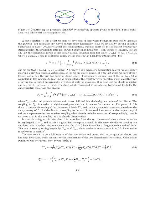
Figure 15: Constructing the projective plane RP 2 by identifying opposite points on the disk. This is equivalent
to a sphere with a crosscap insertion.
A first objection to this is that we seem to have cheated somewhat: Strings are supposed to generate
the graviton (and ultimately any curved backgrounds) dynamically. Have we cheated by putting in such a
background by hand? Or a more careful, less confrontational question might be: Is it consistent with the way
strings generate the graviton to introduce curved backgrounds in this way? Well, let us see. Imagine, to start
off, that the background metric is only locally a small deviation from flat space: Gµν(X) = ηµν + hµν(X),
where h is small. Then, in conformal gauge, we can write in the Euclidean path integral (26):
e −Sσ = e −S
1 + 1
4πα ′
d 2 zhµν(X)∂zX µ ∂¯zX ν
+ . . . , (92)
and we see that if hµν(X) ∝ gsζµν exp(ik · X), where ζ is a symmetric polarization matrix, we are simply
inserting a graviton emission vertex operator. So we are indeed consistent with that which we have already
learned about how the graviton arises in string theory. Furthermore, the insertion of the full Gµν(X) is
equivalent in this language to inserting an exponential of the graviton vertex operator, which is another way
of saying that a curved background is a “coherent state” of gravitons. It is clear that we should generalise
our success, by including σ–model couplings which correspond to introducing background fields for the
antisymmetric tensor and the dilaton:
Sσ = 1
4πα ′
d 2 σ g 1/2 (g ab Gµν(X) + iɛ ab Bµν(X))∂aX µ ∂bX ν + α ′ ΦR , (93)
where Bµν is the background antisymmetric tensor field and Φ is the background value of the dilaton. The
coupling for Bµν is a rather straightforward generalisation of the case for the metric. The power of α ′ is
there to counter the scaling of the dimension 1 fields X µ , and the antisymmetric tensor accommodates the
antisymmetry of B. For the dilaton, a coupling to the two dimensional Ricci scalar is the simplest way of
writing a reparameterisation invariant coupling when there is no index structure. Correspondingly, there is
no power of α ′ in this coupling, as it is already dimensionless.
It is worth noting at this point that α ′ is rather like ¯h for this two dimensional theory, since the action
is very large if α ′ → 0, and so this is a good limit to expand around. In this sense, the dilaton coupling is a
one–loop term. Another thing to notice is that the α ′ → 0 limit is also like a “large spacetime radius” limit.
This can be seen by scaling lengths by Gµν → r 2 Gµν, which results in an expansion in α ′ /r 2 . Large radius
is equivalent to small α ′ .
The next step is to do a full analysis of this new action and ensure that in the quantum theory, one
has Weyl invariance, which amounts to the tracelessness of the two dimensional stress tensor. Calculations
(which we will not discuss here) reveal that[1, 2]:
T a a = − 1
2α ′ βG µνg ab ∂aX µ ∂bX ν − i
2α ′ βB µνɛ ab ∂aX µ ∂bX ν − 1
2 βΦ R . (94)
β G µν = α ′
Rµν + 2∇µ∇νΦ − 1 κσ
HµκσHν 4
26
+ O(α ′2 ),