Introduction to String Theory and D–Branes - School of Natural ...
Introduction to String Theory and D–Branes - School of Natural ...
Introduction to String Theory and D–Branes - School of Natural ...

You also want an ePaper? Increase the reach of your titles
YUMPU automatically turns print PDFs into web optimized ePapers that Google loves.
<strong>Introduction</strong> <strong>to</strong> <strong>String</strong> <strong>Theory</strong> <strong>and</strong> <strong>D–Branes</strong><br />
Clifford V. Johnson<br />
Department <strong>of</strong> Physics <strong>and</strong> Astronomy<br />
University <strong>of</strong> Southern California<br />
Los Angeles, CA 90089–0484, U.S.A.<br />
johnson1@usc.edu<br />
28th March 2004<br />
Abstract<br />
These lecture notes cover a number <strong>of</strong> introduc<strong>to</strong>ry <strong>to</strong>pics in the area <strong>of</strong> string theory, <strong>and</strong> are<br />
intended as a foundation for many <strong>of</strong> the other lecture courses in TASI 2003. The st<strong>and</strong>ard <strong>to</strong>pics in<br />
perturbative string theory are covered, including some basic conformal field theory, T–Duality <strong>and</strong> D–<br />
Branes. Some <strong>of</strong> the properties <strong>of</strong> the latter are uncovered using various techniques. Some st<strong>and</strong>ard<br />
properties <strong>of</strong> supersymmetric strings at strong coupling are reviewed, focusing on the role which branes<br />
play in uncovering those properties.<br />
Contents<br />
1 Introduc<strong>to</strong>ry Remarks 4<br />
2 Relativistic <strong>String</strong>s 5<br />
2.1 Classical Bosonic <strong>String</strong>s . . . . . . . . . . . . . . . . . . . . . . . . . . . . . . . . . . . . . . . 5<br />
2.1.1 Two Actions . . . . . . . . . . . . . . . . . . . . . . . . . . . . . . . . . . . . . . . . . 5<br />
2.2 <strong>String</strong> Equations <strong>of</strong> Motion . . . . . . . . . . . . . . . . . . . . . . . . . . . . . . . . . . . . . 8<br />
2.3 Further Aspects <strong>of</strong> the Two–Dimensional Perspective . . . . . . . . . . . . . . . . . . . . . . . 9<br />
2.3.1 The Stress Tensor . . . . . . . . . . . . . . . . . . . . . . . . . . . . . . . . . . . . . . 10<br />
2.4 Gauge Fixing . . . . . . . . . . . . . . . . . . . . . . . . . . . . . . . . . . . . . . . . . . . . . 10<br />
2.4.1 The Mode Decomposition . . . . . . . . . . . . . . . . . . . . . . . . . . . . . . . . . . 11<br />
2.5 Conformal Invariance . . . . . . . . . . . . . . . . . . . . . . . . . . . . . . . . . . . . . . . . . 12<br />
2.5.1 Some Hamil<strong>to</strong>nian Dynamics . . . . . . . . . . . . . . . . . . . . . . . . . . . . . . . . 12<br />
2.6 Quantised Bosonic <strong>String</strong>s . . . . . . . . . . . . . . . . . . . . . . . . . . . . . . . . . . . . . . 14<br />
2.7 The Constraints <strong>and</strong> Physical States . . . . . . . . . . . . . . . . . . . . . . . . . . . . . . . . 14<br />
2.7.1 The Intercept <strong>and</strong> Critical Dimensions . . . . . . . . . . . . . . . . . . . . . . . . . . . 15<br />
2.8 A Glance at More Sophisticated Techniques . . . . . . . . . . . . . . . . . . . . . . . . . . . . 17<br />
2.9 The Sphere, the Plane <strong>and</strong> the Vertex Opera<strong>to</strong>r . . . . . . . . . . . . . . . . . . . . . . . . . . 18<br />
2.9.1 Zero Point Energy From the Exponential Map . . . . . . . . . . . . . . . . . . . . . . 20<br />
2.9.2 States <strong>and</strong> Opera<strong>to</strong>rs . . . . . . . . . . . . . . . . . . . . . . . . . . . . . . . . . . . . . 20<br />
2.10 Chan–Pa<strong>to</strong>n Fac<strong>to</strong>rs . . . . . . . . . . . . . . . . . . . . . . . . . . . . . . . . . . . . . . . . . 22<br />
2.11 Unoriented <strong>String</strong>s . . . . . . . . . . . . . . . . . . . . . . . . . . . . . . . . . . . . . . . . . . 23<br />
2.11.1 Unoriented Open <strong>String</strong>s . . . . . . . . . . . . . . . . . . . . . . . . . . . . . . . . . . 23<br />
2.11.2 Unoriented Closed <strong>String</strong>s . . . . . . . . . . . . . . . . . . . . . . . . . . . . . . . . . . 24<br />
1
2.12 World–sheet Diagrams . . . . . . . . . . . . . . . . . . . . . . . . . . . . . . . . . . . . . . . . 24<br />
2.13 <strong>String</strong>s in Curved Backgrounds . . . . . . . . . . . . . . . . . . . . . . . . . . . . . . . . . . . 25<br />
2.14 A Quick Look at Geometry . . . . . . . . . . . . . . . . . . . . . . . . . . . . . . . . . . . . . 28<br />
2.14.1 Working with the Local Tangent Frames . . . . . . . . . . . . . . . . . . . . . . . . . . 28<br />
2.14.2 Coordinate vs. Orthonormal Bases . . . . . . . . . . . . . . . . . . . . . . . . . . . . . 29<br />
2.14.3 The Lorentz Group as a Gauge Group . . . . . . . . . . . . . . . . . . . . . . . . . . . 30<br />
2.14.4 Fermions in Curved Spacetime . . . . . . . . . . . . . . . . . . . . . . . . . . . . . . . 30<br />
2.14.5 Comparison <strong>to</strong> Differential Geometry . . . . . . . . . . . . . . . . . . . . . . . . . . . . 31<br />
3 A Closer Look at the World–Sheet 31<br />
3.1 Conformal Invariance . . . . . . . . . . . . . . . . . . . . . . . . . . . . . . . . . . . . . . . . . 31<br />
3.1.1 Diverse Dimensions . . . . . . . . . . . . . . . . . . . . . . . . . . . . . . . . . . . . . . 32<br />
3.2 The Special Case <strong>of</strong> Two Dimensions . . . . . . . . . . . . . . . . . . . . . . . . . . . . . . . . 33<br />
3.2.1 States <strong>and</strong> Opera<strong>to</strong>rs . . . . . . . . . . . . . . . . . . . . . . . . . . . . . . . . . . . . . 34<br />
3.3 The Opera<strong>to</strong>r Product Expansion . . . . . . . . . . . . . . . . . . . . . . . . . . . . . . . . . . 35<br />
3.3.1 The Stress Tensor <strong>and</strong> the Virasoro Algebra . . . . . . . . . . . . . . . . . . . . . . . . 35<br />
3.4 Revisiting the Relativistic <strong>String</strong> . . . . . . . . . . . . . . . . . . . . . . . . . . . . . . . . . . 38<br />
3.5 Fixing The Conformal Gauge . . . . . . . . . . . . . . . . . . . . . . . . . . . . . . . . . . . . 41<br />
3.5.1 Conformal Ghosts . . . . . . . . . . . . . . . . . . . . . . . . . . . . . . . . . . . . . . 41<br />
3.5.2 The Critical Dimension . . . . . . . . . . . . . . . . . . . . . . . . . . . . . . . . . . . 42<br />
3.5.3 Further Aspects <strong>of</strong> Conformal Ghosts . . . . . . . . . . . . . . . . . . . . . . . . . . . 43<br />
3.6 Non–Critical <strong>String</strong>s . . . . . . . . . . . . . . . . . . . . . . . . . . . . . . . . . . . . . . . . . 43<br />
3.7 The Closed <strong>String</strong> Partition Function . . . . . . . . . . . . . . . . . . . . . . . . . . . . . . . . 45<br />
4 <strong>String</strong>s on Circles <strong>and</strong> T–Duality 48<br />
4.1 Closed <strong>String</strong>s on a Circle . . . . . . . . . . . . . . . . . . . . . . . . . . . . . . . . . . . . . . 48<br />
4.2 T–Duality for Closed <strong>String</strong>s . . . . . . . . . . . . . . . . . . . . . . . . . . . . . . . . . . . . 50<br />
4.3 A Special Radius: Enhanced Gauge Symmetry . . . . . . . . . . . . . . . . . . . . . . . . . . 50<br />
4.4 The Circle Partition Function . . . . . . . . . . . . . . . . . . . . . . . . . . . . . . . . . . . . 51<br />
4.4.1 Affine Lie Algebras . . . . . . . . . . . . . . . . . . . . . . . . . . . . . . . . . . . . . . 52<br />
4.5 Toriodal Compactifications . . . . . . . . . . . . . . . . . . . . . . . . . . . . . . . . . . . . . 53<br />
4.5.1 The Moduli Space <strong>of</strong> Compactifications . . . . . . . . . . . . . . . . . . . . . . . . . . 55<br />
4.6 Another Special Radius: Bosonisation . . . . . . . . . . . . . . . . . . . . . . . . . . . . . . . 55<br />
4.7 <strong>String</strong> <strong>Theory</strong> on an Orbifold . . . . . . . . . . . . . . . . . . . . . . . . . . . . . . . . . . . . 58<br />
4.8 T–Duality for Open <strong>String</strong>s: D–branes . . . . . . . . . . . . . . . . . . . . . . . . . . . . . . . 59<br />
4.9 Chan–Pa<strong>to</strong>n Fac<strong>to</strong>rs <strong>and</strong> Wilson Lines . . . . . . . . . . . . . . . . . . . . . . . . . . . . . . . 60<br />
4.10 D–Brane Collective Coördinates . . . . . . . . . . . . . . . . . . . . . . . . . . . . . . . . . . . 62<br />
4.11 T–Duality for Unoriented <strong>String</strong>s . . . . . . . . . . . . . . . . . . . . . . . . . . . . . . . . . . 64<br />
4.11.1 Orientifolds. . . . . . . . . . . . . . . . . . . . . . . . . . . . . . . . . . . . . . . . . . . 64<br />
4.11.2 Orientifolds <strong>and</strong> <strong>D–Branes</strong> . . . . . . . . . . . . . . . . . . . . . . . . . . . . . . . . . . 65<br />
5 Background Fields <strong>and</strong> World–Volume Actions 66<br />
5.1 T–duality in Background Fields . . . . . . . . . . . . . . . . . . . . . . . . . . . . . . . . . . . 66<br />
5.2 A First Look at the D–brane World–Volume Action . . . . . . . . . . . . . . . . . . . . . . . 67<br />
5.2.1 World–Volume Actions from Tilted <strong>D–Branes</strong> . . . . . . . . . . . . . . . . . . . . . . . 69<br />
5.3 The Dirac–Born–Infeld Action . . . . . . . . . . . . . . . . . . . . . . . . . . . . . . . . . . . 69<br />
5.4 The Action <strong>of</strong> T–Duality . . . . . . . . . . . . . . . . . . . . . . . . . . . . . . . . . . . . . . . 70<br />
5.5 Non–Abelian Extensions . . . . . . . . . . . . . . . . . . . . . . . . . . . . . . . . . . . . . . . 71<br />
5.6 <strong>D–Branes</strong> <strong>and</strong> Gauge <strong>Theory</strong> . . . . . . . . . . . . . . . . . . . . . . . . . . . . . . . . . . . . 71<br />
5.7 BPS Lumps on the World–volume . . . . . . . . . . . . . . . . . . . . . . . . . . . . . . . . . 72<br />
2
6 D–Brane Tension <strong>and</strong> Boundary States 73<br />
6.1 The D–brane Tension . . . . . . . . . . . . . . . . . . . . . . . . . . . . . . . . . . . . . . . . 74<br />
6.1.1 An Open <strong>String</strong> Partition Function . . . . . . . . . . . . . . . . . . . . . . . . . . . . . 74<br />
6.2 A Background Field Computation . . . . . . . . . . . . . . . . . . . . . . . . . . . . . . . . . 76<br />
6.3 The Orientifold Tension . . . . . . . . . . . . . . . . . . . . . . . . . . . . . . . . . . . . . . . 77<br />
6.3.1 Another Open <strong>String</strong> Partition Function . . . . . . . . . . . . . . . . . . . . . . . . . . 77<br />
6.4 The Boundary State Formalism . . . . . . . . . . . . . . . . . . . . . . . . . . . . . . . . . . . 79<br />
7 Supersymmetric <strong>String</strong>s 81<br />
7.1 The Three Basic Superstring Theories . . . . . . . . . . . . . . . . . . . . . . . . . . . . . . . 81<br />
7.1.1 Open Superstrings: Type I . . . . . . . . . . . . . . . . . . . . . . . . . . . . . . . . . 81<br />
7.1.2 Gauge <strong>and</strong> Gravitational Anomalies . . . . . . . . . . . . . . . . . . . . . . . . . . . . 85<br />
7.1.3 The Chern–Simons Three–Form . . . . . . . . . . . . . . . . . . . . . . . . . . . . . . 85<br />
7.1.4 A list <strong>of</strong> Anomaly Polynomials . . . . . . . . . . . . . . . . . . . . . . . . . . . . . . . 86<br />
7.2 Closed Superstrings: Type II . . . . . . . . . . . . . . . . . . . . . . . . . . . . . . . . . . . . 87<br />
7.2.1 Type I from Type IIB, The Pro<strong>to</strong>type Orientifold . . . . . . . . . . . . . . . . . . . . 88<br />
7.3 The Green–Schwarz Mechanism . . . . . . . . . . . . . . . . . . . . . . . . . . . . . . . . . . . 89<br />
7.4 The Two Basic Heterotic <strong>String</strong> Theories . . . . . . . . . . . . . . . . . . . . . . . . . . . . . 91<br />
7.4.1 SO(32) <strong>and</strong> E8 × E8 From Self–Dual Lattices . . . . . . . . . . . . . . . . . . . . . . . 92<br />
7.5 The Massless Spectrum . . . . . . . . . . . . . . . . . . . . . . . . . . . . . . . . . . . . . . . 93<br />
7.6 The Ten Dimensional Supergravities . . . . . . . . . . . . . . . . . . . . . . . . . . . . . . . . 93<br />
7.7 Heterotic Toroidal Compactifications . . . . . . . . . . . . . . . . . . . . . . . . . . . . . . . . 95<br />
7.8 Superstring Toroidal Compactification . . . . . . . . . . . . . . . . . . . . . . . . . . . . . . . 96<br />
7.9 A Superstring Orbifold: The K3 Manifold . . . . . . . . . . . . . . . . . . . . . . . . . . . . . 97<br />
7.9.1 The Orbifold Spectrum . . . . . . . . . . . . . . . . . . . . . . . . . . . . . . . . . . . 97<br />
7.9.2 Another Miraculous Anomaly Cancellation . . . . . . . . . . . . . . . . . . . . . . . . 99<br />
7.9.3 The K3 Manifold . . . . . . . . . . . . . . . . . . . . . . . . . . . . . . . . . . . . . . . 100<br />
7.9.4 Blowing Up the Orbifold . . . . . . . . . . . . . . . . . . . . . . . . . . . . . . . . . . . 100<br />
7.9.5 Anticipating a <strong>String</strong>/<strong>String</strong> Duality in D = 6 . . . . . . . . . . . . . . . . . . . . . . 102<br />
8 Supersymmetric <strong>String</strong>s <strong>and</strong> T–Duality 102<br />
8.1 T–Duality <strong>of</strong> Supersymmetric <strong>String</strong>s . . . . . . . . . . . . . . . . . . . . . . . . . . . . . . . 102<br />
8.1.1 T–Duality <strong>of</strong> Type II Superstrings . . . . . . . . . . . . . . . . . . . . . . . . . . . . . 103<br />
8.1.2 T–Duality <strong>of</strong> Type I Superstrings . . . . . . . . . . . . . . . . . . . . . . . . . . . . . . 103<br />
8.1.3 T–duality for the Heterotic <strong>String</strong>s . . . . . . . . . . . . . . . . . . . . . . . . . . . . . 104<br />
8.2 <strong>D–Branes</strong> as BPS Soli<strong>to</strong>ns . . . . . . . . . . . . . . . . . . . . . . . . . . . . . . . . . . . . . . 105<br />
8.2.1 A Summary <strong>of</strong> Forms <strong>and</strong> Branes . . . . . . . . . . . . . . . . . . . . . . . . . . . . . . 105<br />
8.3 The D–Brane Charge <strong>and</strong> Tension . . . . . . . . . . . . . . . . . . . . . . . . . . . . . . . . . 106<br />
8.4 The Orientifold Charge <strong>and</strong> Tension . . . . . . . . . . . . . . . . . . . . . . . . . . . . . . . . 108<br />
8.5 Type I from Type IIB, Revisited . . . . . . . . . . . . . . . . . . . . . . . . . . . . . . . . . . 108<br />
8.6 Dirac Charge Quantization . . . . . . . . . . . . . . . . . . . . . . . . . . . . . . . . . . . . . 108<br />
8.7 <strong>D–Branes</strong> in Type I . . . . . . . . . . . . . . . . . . . . . . . . . . . . . . . . . . . . . . . . . 109<br />
9 World–Volume Curvature Couplings 110<br />
9.1 Tilted <strong>D–Branes</strong> <strong>and</strong> Branes within Branes . . . . . . . . . . . . . . . . . . . . . . . . . . . . 111<br />
9.2 Anomalous Gauge Couplings . . . . . . . . . . . . . . . . . . . . . . . . . . . . . . . . . . . . 111<br />
9.2.1 The Dirac Monopole as a Gauge Bundle . . . . . . . . . . . . . . . . . . . . . . . . . . 113<br />
9.3 Characteristic Classes <strong>and</strong> Invariant Polynomials . . . . . . . . . . . . . . . . . . . . . . . . . 114<br />
9.4 Anomalous Curvature Couplings . . . . . . . . . . . . . . . . . . . . . . . . . . . . . . . . . . 117<br />
9.5 A Relation <strong>to</strong> Anomalies . . . . . . . . . . . . . . . . . . . . . . . . . . . . . . . . . . . . . . . 118<br />
9.6 D–branes <strong>and</strong> K–<strong>Theory</strong> . . . . . . . . . . . . . . . . . . . . . . . . . . . . . . . . . . . . . . . 120<br />
3
9.7 Further Non–Abelian Extensions . . . . . . . . . . . . . . . . . . . . . . . . . . . . . . . . . . 120<br />
9.8 Further Curvature Couplings . . . . . . . . . . . . . . . . . . . . . . . . . . . . . . . . . . . . 121<br />
10 Multiple <strong>D–Branes</strong> 122<br />
10.1 Dp <strong>and</strong> Dp ′ From Boundary Conditions . . . . . . . . . . . . . . . . . . . . . . . . . . . . . . 122<br />
10.2 The BPS Bound for the Dp–Dp ′ System . . . . . . . . . . . . . . . . . . . . . . . . . . . . . . 124<br />
10.3 Bound States <strong>of</strong> Fundamental <strong>String</strong>s <strong>and</strong> D–<strong>String</strong>s . . . . . . . . . . . . . . . . . . . . . . . 125<br />
10.4 The Three–<strong>String</strong> Junction . . . . . . . . . . . . . . . . . . . . . . . . . . . . . . . . . . . . . 126<br />
10.5 Aspects <strong>of</strong> D–Brane Bound States . . . . . . . . . . . . . . . . . . . . . . . . . . . . . . . . . 128<br />
10.5.1 0–0 bound states . . . . . . . . . . . . . . . . . . . . . . . . . . . . . . . . . . . . . . . 128<br />
10.5.2 0–2 bound states . . . . . . . . . . . . . . . . . . . . . . . . . . . . . . . . . . . . . . . 128<br />
10.5.3 0–4 bound states . . . . . . . . . . . . . . . . . . . . . . . . . . . . . . . . . . . . . . . 128<br />
10.5.4 0–6 bound states . . . . . . . . . . . . . . . . . . . . . . . . . . . . . . . . . . . . . . . 129<br />
10.5.5 0–8 bound states . . . . . . . . . . . . . . . . . . . . . . . . . . . . . . . . . . . . . . . 129<br />
11 <strong>String</strong>s at Strong Coupling 129<br />
11.1 Type IIB/Type IIB Duality . . . . . . . . . . . . . . . . . . . . . . . . . . . . . . . . . . . . . 129<br />
11.1.1 D1–Brane Collective Coordinates . . . . . . . . . . . . . . . . . . . . . . . . . . . . . 129<br />
11.1.2 S–Duality <strong>and</strong> SL(2, Z) . . . . . . . . . . . . . . . . . . . . . . . . . . . . . . . . . . . 131<br />
11.2 SO(32) Type I/Heterotic Duality . . . . . . . . . . . . . . . . . . . . . . . . . . . . . . . . . . 131<br />
11.2.1 D1–Brane Collective Coordinates . . . . . . . . . . . . . . . . . . . . . . . . . . . . . 131<br />
11.3 Dual Branes from 10D <strong>String</strong>–<strong>String</strong> Duality . . . . . . . . . . . . . . . . . . . . . . . . . . . 132<br />
11.3.1 The Heterotic NS–Fivebrane . . . . . . . . . . . . . . . . . . . . . . . . . . . . . . . . 133<br />
11.3.2 The Type IIA <strong>and</strong> Type IIB NS5–brane . . . . . . . . . . . . . . . . . . . . . . . . . . 133<br />
11.4 Type IIA/M–<strong>Theory</strong> Duality . . . . . . . . . . . . . . . . . . . . . . . . . . . . . . . . . . . . 135<br />
11.4.1 A Closer Look at D0–branes . . . . . . . . . . . . . . . . . . . . . . . . . . . . . . . . 135<br />
11.4.2 Eleven Dimensional Supergravity . . . . . . . . . . . . . . . . . . . . . . . . . . . . . 136<br />
11.5 E8 × E8 Heterotic <strong>String</strong>/M–<strong>Theory</strong> Duality . . . . . . . . . . . . . . . . . . . . . . . . . . . 137<br />
11.6 M2–branes <strong>and</strong> M5–branes . . . . . . . . . . . . . . . . . . . . . . . . . . . . . . . . . . . . . 138<br />
11.6.1 From <strong>D–Branes</strong> <strong>and</strong> NS5–branes <strong>to</strong> M–Branes <strong>and</strong> Back . . . . . . . . . . . . . . . . 139<br />
11.7 U–Duality . . . . . . . . . . . . . . . . . . . . . . . . . . . . . . . . . . . . . . . . . . . . . . . 139<br />
11.7.1 Type II <strong>String</strong>s on T 5 <strong>and</strong> E 6(6) . . . . . . . . . . . . . . . . . . . . . . . . . . . . . . 139<br />
12 Concluding Remarks 141<br />
References 141<br />
1 Introduc<strong>to</strong>ry Remarks<br />
These lectures are intended <strong>to</strong> serve as an introduction <strong>to</strong> some <strong>of</strong> the basic techniques, language <strong>and</strong> concepts<br />
in string theory <strong>and</strong> D–branes. by no stretch <strong>of</strong> the imagination will you learn everything about these <strong>to</strong>pics<br />
from these notes. You should be able <strong>to</strong> use them <strong>to</strong> get a good sense for how things work, <strong>and</strong> this will<br />
allow you <strong>to</strong> underst<strong>and</strong> the issues which are discussed in the other lecture courses in this school, which will<br />
assume a knowledge <strong>of</strong> basic string theory, <strong>and</strong> some previous experience with some <strong>of</strong> the “post–Second–<br />
Revolution” ideas. Once you get <strong>to</strong> a certain stage, the notes will need <strong>to</strong> be supplemented with more careful<br />
treatments <strong>of</strong> the technology, <strong>and</strong> you will be curious <strong>to</strong> know more about some <strong>of</strong> the <strong>to</strong>pics <strong>and</strong> further<br />
applications that I did not have time or space <strong>to</strong> cover here. I recommend the excellent text <strong>of</strong> Polchinski[1],<br />
<strong>and</strong> also that <strong>of</strong> Green, Schwarz <strong>and</strong> Witten[2], which is still a brilliant text for many aspects <strong>of</strong> the subject.<br />
You might want <strong>to</strong> consult the recent book listed in ref.[4], in order <strong>to</strong> learn more about D–branes <strong>and</strong><br />
4
further aspects <strong>of</strong> their applications. There are also many other sources, on the web (e.g., www.arXiv.org)<br />
<strong>and</strong> elsewhere, <strong>of</strong> detailed reviews <strong>of</strong> various specialized <strong>to</strong>pics, even whole string theory books[3].<br />
These notes grew out <strong>of</strong> a series <strong>of</strong> notes, including those <strong>of</strong> ref.[5, 6, 7, 8], <strong>and</strong> I have also borrowed<br />
from parts <strong>of</strong> the book “<strong>D–Branes</strong>”[4]. I’ve included the basic material on stings <strong>and</strong> T–duality, <strong>and</strong> tried <strong>to</strong><br />
include a little more <strong>of</strong> the conformal field theory language than I have used before in notes <strong>of</strong> this sort. It<br />
allows the language <strong>of</strong> the study <strong>of</strong> <strong>to</strong>roidal compactification <strong>to</strong> be developed quite efficiently <strong>and</strong> (I hope)<br />
clearly. The pay<strong>of</strong>f is that is becomes easier <strong>to</strong> see how the heterotic strings work, <strong>and</strong> how they fit in with<br />
the other strings quite nicely. Furthermore, it allows one <strong>to</strong> explain a little about non–critical strings, a<br />
<strong>to</strong>pic <strong>of</strong> considerable interest. It also sets up the important language used in string compactifications, <strong>and</strong><br />
prepares one for concepts such as U–duality later on. There’s a <strong>to</strong>uch more geometry covered than I usually<br />
do, such as some basic <strong>to</strong>ols for working on the tangent space any curved spacetime manifold. This comes<br />
in<strong>to</strong> its own in later sections when I describe the anomalies which arise in the low energy effective actions <strong>of</strong><br />
the various superstrings. The Green–Schwarz anomaly cancellation mechanism (the foundation <strong>of</strong> the First<br />
Revolution) is studied in gory detail. This is done for fun in section 6, but there is a bonus in section 8 when<br />
we look a bit more closely at gauge bundles <strong>and</strong> characteristic classes, allowing us <strong>to</strong> revisit the language<br />
<strong>of</strong> anomalies, now on the world–volumes <strong>of</strong> D–branes. The Green–Schwarz mechanism is then seen <strong>to</strong> be a<br />
basic paradigm for how extended objects with interesting massless fields on their world–volumes actually fit<br />
in<strong>to</strong> the various field theories. I suspect that there will be some resonance with the lectures <strong>of</strong> Jeff Harvey<br />
in this area.<br />
There is the obliga<strong>to</strong>ry section on strings at strong coupling. I’ve put in the st<strong>and</strong>ard classic D–brane<br />
probes <strong>of</strong> the duality, <strong>and</strong> outlined other aspects <strong>of</strong> how the D–branes get involved in the whole s<strong>to</strong>ry,<br />
including how you can deduce the existence <strong>of</strong> other important branes, the NS5–branes <strong>and</strong> the M–branes.<br />
This is important basic lore, but I don’t go <strong>to</strong>o far in<strong>to</strong> this treatment in order <strong>to</strong> save space. There are<br />
plenty <strong>of</strong> excellent reviews <strong>of</strong> this material in the literature I’ve already mentioned, <strong>and</strong> also in (for example)<br />
ref.[175].<br />
I’ve included a table <strong>of</strong> contents for you which might help make this a useful reference. Enjoy, —cvj.<br />
2 Relativistic <strong>String</strong>s<br />
This section is devoted <strong>to</strong> an introduction <strong>to</strong> bosonic strings <strong>and</strong> their quantization. There is no attempt<br />
made at performing a rigourous or exhaustive derivation <strong>of</strong> some <strong>of</strong> the various formulae we will encounter,<br />
since that would take us well away from the main goal. That goal is <strong>to</strong> underst<strong>and</strong> some <strong>of</strong> how string theory<br />
incorporates some <strong>of</strong> the familiar spacetime physics that we know from low energy field theory, <strong>and</strong> then<br />
rapidly proceed <strong>to</strong> the point where many <strong>of</strong> the remarkable properties which make strings so different from<br />
field theory are manifest. That will be a good foundation for appreciating just what D–branes really are.<br />
The careful reader who needs <strong>to</strong> know more <strong>of</strong> the details behind some <strong>of</strong> what we will introduce is invited<br />
<strong>to</strong> consult texts devoted <strong>to</strong> the study <strong>of</strong> string theory.<br />
2.1 Classical Bosonic <strong>String</strong>s<br />
Turning <strong>to</strong> strings, we parameterize the “world–sheet” which the string sweeps out with coordinates (σ 1 , σ 2 ) =<br />
(τ, σ). The latter is a spatial coordinate, <strong>and</strong> for now, we take the string <strong>to</strong> be an open one, with 0 ≤ σ ≤ π<br />
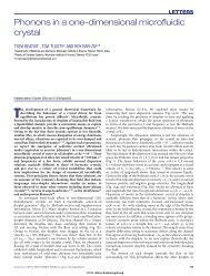
running from one end <strong>to</strong> the other. The string’s evolution in spacetime is described by the functions X µ (τ, σ),<br />
µ = 0, · · ·,D − 1, giving the shape <strong>of</strong> the string’s world–sheet in target spacetime (see figure 1).<br />
2.1.1 Two Actions<br />
A natural object which arises from embedding the string in<strong>to</strong> spacetime using the functions (or “map”)<br />
X µ (τ, σ) is a two dimensional “induced” metric on the world–sheet:<br />
hab = ∂aX µ ∂bX ν ηµν . (1)<br />
5
X 1<br />
0<br />
X<br />
σ<br />
τ<br />
X 2<br />
X µ (τ,σ)<br />
τ<br />
σ<br />
0 π<br />
Figure 1: A string’s world–sheet. The function X µ (τ, σ) embeds the world–sheet, parameterized by (τ, σ),<br />
in<strong>to</strong> spacetime, with coordinates given by X µ .<br />
distances on the world–sheet as an object embedded in spacetime, <strong>and</strong> hence define an action analogous <strong>to</strong><br />
one we would write for a particle: the <strong>to</strong>tal area swept out by the world–sheet:<br />
<br />
So = −T dA = −T dτdσ (−dethab) 1/2 <br />
≡ dτdσ L( ˙ X, X ′ ; σ, τ) . (2)<br />
So<br />
∂X µ ∂X<br />
= −T dτdσ<br />
∂σ<br />
µ 2 µ 2 <br />
2<br />
1/2<br />
∂X ∂Xµ<br />
−<br />
∂τ ∂σ ∂τ<br />
<br />
= −T dτdσ (X ′ · X) ˙ 2 ′2<br />
− X X˙ 2 1/2 , (3)<br />
where X ′ means ∂X/∂σ <strong>and</strong> a dot means differentiation with respect <strong>to</strong> τ. This is the Nambu–Go<strong>to</strong> action.<br />
T is the tension <strong>of</strong> the string, which has dimensions <strong>of</strong> inverse squared length.<br />
Varying the action, we have generally:<br />
δSo =<br />
<br />
∂L<br />
dτdσ<br />
∂ ˙ X µδ ˙ X µ + ∂L<br />
=<br />
<br />
′µ<br />
∂X ′µδX<br />
<br />
dτdσ − ∂ ∂L<br />
∂τ ∂ ˙ ∂ ∂L<br />
−<br />
X µ ∂σ ∂X ′µ<br />
<br />
δX µ <br />
+<br />
Requiring this <strong>to</strong> be zero, we get:<br />
∂ ∂L<br />
∂τ ∂ ˙ ∂ ∂L<br />
+ = 0 <strong>and</strong><br />
X µ ∂σ ∂X ′µ<br />
which are statements about the conjugate momenta:<br />
∂<br />
∂τ P µ τ<br />
+ ∂<br />
∂σ P µ σ = 0 <strong>and</strong> P µ σ<br />
dτ<br />
<br />
∂L σ=π<br />
′µ<br />
∂X ′µδX<br />
σ=0<br />
. (4)<br />
∂L<br />
= 0 at σ = 0, π , (5)<br />
∂X ′µ<br />
= 0 at σ = 0, π . (6)<br />
Here, P µ σ is the momentum running along the string (i.e., in the σ direction) while P µ τ is the momentum<br />
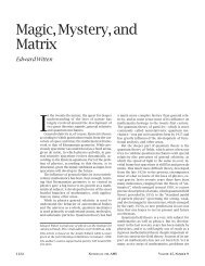
running transverse <strong>to</strong> it. The <strong>to</strong>tal spacetime momentum is given by integrating up the infinitesimal (see<br />
figure 2):<br />
dP µ = P µ τ dσ + P µ σ dτ . (7)<br />
6
µ<br />
Pσ dσ<br />
Figure 2: The infinitesimal momenta on the world sheet.<br />
Actually, we can choose any slice <strong>of</strong> the world–sheet in order <strong>to</strong> compute this momentum. A most convenient<br />
one is a slice τ = constant, revealing the string in its original paramaterization: P µ = P µ τ dσ, but any other<br />
slice will do.<br />
Similarly, one can define the angular momentum:<br />
M µν <br />
= (P µ τ X ν − P ν τ X µ )dσ . (8)<br />
It is a simple exercise <strong>to</strong> work out the momenta for our particular Lagrangian:<br />
It is interesting <strong>to</strong> compute the square <strong>of</strong> P µ σ<br />
P µ<br />
τ<br />
dτ<br />
P µ τ = T ˙ X µ X ′2 − X ′µ ( ˙ X · X ′ )<br />
<br />
( ˙ X · X ′ ) 2 − ˙ X2X ′2<br />
P µ σ = T X′µ X˙ 2 − X ˙ µ ( X ˙ ′ · X )<br />
<br />
( ˙ X · X ′ ) 2 − ˙ X2X ′2<br />
from this expression, <strong>and</strong> one finds that<br />
. (9)<br />
P 2 σ ≡ P µ σ Pµσ = −2T 2 ˙ X 2 . (10)<br />
This is our first (perhaps) non–intuitive classical result. We noticed that Pσ vanishes at the endpoints, in<br />
order <strong>to</strong> prevent momentum from flowing <strong>of</strong>f the ends <strong>of</strong> the string. The equation we just derived implies<br />
that ˙ X 2 = 0 at the endpoints, which is <strong>to</strong> say that they move at the speed <strong>of</strong> light.<br />
We can introduce an equivalent action which does not have the square root form that the current one<br />
has. Once again, we do it by introducing a independent metric, γab(σ, τ), on the world–sheet, <strong>and</strong> write the<br />
“Polyakov” action:<br />
If we vary γ, we get<br />
δS = − 1<br />
4πα ′<br />
<br />
S = − 1<br />
4πα ′<br />
<br />
= − 1<br />
4πα ′<br />
d 2 σ<br />
Using the fact that δγ = γγ ab δγab = −γγabδγ ab , we get<br />
δS = − 1<br />
4πα ′<br />
<br />
<br />
dτdσ(−γ) 1/2 γ ab ∂aX µ ∂bX ν ηµν<br />
d 2 σ (−γ) 1/2 γ ab hab . (11)<br />
<br />
− 1<br />
2 (−γ)1/2δγγ ab hab + (−γ) 1/2 δγ ab <br />
hab<br />
d 2 σ (−γ) 1/2 δγ ab<br />
7<br />
<br />
hab − 1<br />
2 γabγ cd <br />
hcd<br />
. (12)<br />
. (13)
Therefore we have<br />
from which we can derive<br />
<strong>and</strong> so substituting in<strong>to</strong> S, we recover the Nambu–Go<strong>to</strong> action, So.<br />
Let us note some <strong>of</strong> the symmetries <strong>of</strong> the action:<br />
• Spacetime Lorentz/Poincaré:<br />
hab − 1<br />
2 γabγ cd hcd = 0 , (14)<br />
γ ab hab = 2(−h) 1/2 (−γ) −1/2 , (15)<br />
X µ → X ′µ = Λ µ νX ν + A µ ,<br />
where Λ is an SO(1, D − 1) Lorentz matrix <strong>and</strong> A µ is an arbitrary constant D–vec<strong>to</strong>r. Just as before<br />
this is a trivial global symmetry <strong>of</strong> S (<strong>and</strong> also So), following from the fact that we wrote them in<br />
covariant form.<br />
• Worldsheet Reparametrisations:<br />
δX µ = ζ a ∂aX µ<br />
δγ ab = ζ c ∂cγ ab − ∂cζ a γ cb − ∂cζ b γ ac , (16)<br />
for two parameters ζ a (τ, σ). This is a non–trivial local or “gauge” symmetry <strong>of</strong> S. This is a large extra<br />
symmetry on the world–sheet <strong>of</strong> which we will make great use.<br />
• Weyl invariance:<br />
γab → γ ′ ab = e2ω γab , (17)<br />
specified by a function ω(τ, σ). This ability <strong>to</strong> do local rescalings <strong>of</strong> the metric results from the fact<br />
that we did not have <strong>to</strong> choose an overall scale when we chose γ ab <strong>to</strong> rewrite So in terms <strong>of</strong> S. This<br />
can be seen especially if we rewrite the relation (15) as (−h) −1/2 hab = (−γ) −1/2 γab.<br />
We note here for future use that there are just as many parameters needed <strong>to</strong> specify the local symmetries<br />
(three) as there are independent components <strong>of</strong> the world-sheet metric. This is very useful, as we shall see.<br />
2.2 <strong>String</strong> Equations <strong>of</strong> Motion<br />
We can get equations <strong>of</strong> motion for the string by varying our action (11) with respect <strong>to</strong> the X µ :<br />
1<br />
δS =<br />
2πα ′<br />
<br />
d 2 <br />
σ ∂a (−γ) 1/2 γ ab <br />
∂bXµ δX µ<br />
− 1<br />
2πα ′<br />
<br />
dτ (−γ) 1/2 ∂σXµδX µ<br />
<br />
<br />
σ=π<br />
, (18)<br />
σ=0<br />
which results in the equations <strong>of</strong> motion:<br />
<br />
(−γ) 1/2 γ ab ∂bX µ<br />
≡ (−γ) 1/2 ∇ 2 X µ = 0 , (19)<br />
with either:<br />
or:<br />
∂a<br />
X ′µ (τ, 0) = 0<br />
X ′µ <br />
(τ, π) = 0<br />
X ′µ (τ, 0) = X ′µ (τ, π)<br />
X µ (τ, 0) = X µ <br />
(τ, π)<br />
γab(τ, 0) = γab(τ, π)<br />
Open <strong>String</strong><br />
(Neumann b.c.’s)<br />
Closed <strong>String</strong><br />
(periodic b.c.’s)<br />
We shall study the equation <strong>of</strong> motion (19) <strong>and</strong> the accompanying boundary conditions a lot later. We are<br />
going <strong>to</strong> look at the st<strong>and</strong>ard Neumann boundary conditions mostly, <strong>and</strong> then consider the case <strong>of</strong> Dirichlet<br />
conditions later, when we uncover D–branes, using T–duality. Notice that we have taken the liberty <strong>of</strong><br />
introducing closed strings by imposing periodicity.<br />
8<br />
(20)<br />
(21)
2.3 Further Aspects <strong>of</strong> the Two–Dimensional Perspective<br />
The action (11) may be thought <strong>of</strong> as a two dimensional model <strong>of</strong> D bosonic fields X µ (τ, σ). This two<br />
dimensional theory has reparameterisation invariance, as it is constructed using the metric γab(τ, σ) in a<br />
covariant way. It is natural <strong>to</strong> ask whether there are other terms which we might want <strong>to</strong> add <strong>to</strong> the<br />
theory which have similar properties. With some experience from General Relativity two other terms spring<br />
effortlessly <strong>to</strong> mind. One is the Einstein–Hilbert action (supplemented with a boundary term):<br />
χ = 1<br />
4π<br />
<br />
M<br />
d 2 σ (−γ) 1/2 R + 1<br />
2π<br />
<br />
∂M<br />
dsK , (22)<br />
where R is the two–dimensional Ricci scalar on the world–sheet M <strong>and</strong> K is the trace <strong>of</strong> the extrinsic<br />
curvature tensor on the boundary ∂M. The other term is:<br />
Θ = 1<br />
4πα ′<br />
<br />
d 2 σ (−γ) 1/2 , (23)<br />
M<br />
which is the cosmological term. What is their role here? Well, under a Weyl transformation (17), it can be<br />
seen that (−γ) 1/2 → e 2ω (−γ) 1/2 <strong>and</strong> R → e −2ω (R − 2∇ 2 ω), <strong>and</strong> so χ is invariant, (because R changes by a<br />
<strong>to</strong>tal derivative which is canceled by the variation <strong>of</strong> K) but Θ is not.<br />
So we will include χ, but not Θ in what follows. Let us anticipate something that we will do later, which<br />
is <strong>to</strong> work with Euclidean signature <strong>to</strong> help make sense <strong>of</strong> the <strong>to</strong>pological statements <strong>to</strong> follow: γab with<br />
signature (−+) has been replaced by gab with signature (++). Now, since as we said earlier, the full string<br />
action resembles two–dimensional gravity coupled <strong>to</strong> D bosonic “matter” fields X µ , <strong>and</strong> the equations <strong>of</strong><br />
motion are <strong>of</strong> course:<br />
Rab − 1<br />
2 γabR = Tab . (24)<br />
The left h<strong>and</strong> side vanishes identically in two dimensions, <strong>and</strong> so there are no dynamics associated <strong>to</strong><br />
(22). The quantity χ depends only on the <strong>to</strong>pology <strong>of</strong> the world–sheet (it is the Euler number) <strong>and</strong> so will<br />
only matter when comparing world sheets <strong>of</strong> different <strong>to</strong>pology. This will arise when we compare results<br />
from different orders <strong>of</strong> string perturbation theory <strong>and</strong> when we consider interactions.<br />
We can see this in the following: Let us add our new term <strong>to</strong> the action, <strong>and</strong> consider the string action<br />
<strong>to</strong> be:<br />
S =<br />
1<br />
4πα ′<br />
<br />
M<br />
d 2 σ g 1/2 g ab ∂aX µ ∂bXµ<br />
+λ<br />
<br />
1<br />
d<br />
4π M<br />
2 σ g 1/2 R + 1<br />
<br />
dsK<br />
2π ∂M<br />
, (25)<br />
where λ is —for now— <strong>and</strong> arbitrary parameter which we have not fixed <strong>to</strong> any particular value1 . So what<br />
will λ do? Recall that it couples <strong>to</strong> Euler number, so in the full path integral defining the string theory:<br />
<br />
Z = DXDg e −S , (26)<br />
resulting amplitudes will be weighted by a fac<strong>to</strong>r e −λχ , where χ = 2−2h−b−c. Here, h, b, c are the numbers<br />
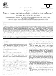
<strong>of</strong> h<strong>and</strong>les, boundaries <strong>and</strong> crosscaps, respectively, on the world sheet. Consider figure 3. An emission <strong>and</strong><br />
reabsorption <strong>of</strong> an open string results in a change δχ = −1, while for a closed string it is δχ = −2. Therefore,<br />
relative <strong>to</strong> the tree level open string diagram (disc <strong>to</strong>pology), the amplitudes are weighted by e λ <strong>and</strong> e 2λ ,<br />
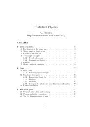
respectively. The quantity gs ≡ e λ therefore will be called the closed string coupling. Note that it is the<br />
square <strong>of</strong> the open string coupling, which justifies the labeling we gave <strong>of</strong> the two three–string diagrams<br />
in figure 4. It is a striking fact that string theory dynamically determines its own coupling strength. (See<br />
figure 4.)<br />
1 Later, it will turn out that λ is not a free parameter. In the full string theory, it has dynamical meaning, <strong>and</strong> will be<br />
equivalent <strong>to</strong> the expectation value <strong>of</strong> one <strong>of</strong> the massless fields —the “dila<strong>to</strong>n”— described by the string.<br />
9
δχ = −2<br />
δχ = −1<br />
Figure 3: World–sheet <strong>to</strong>pology change due <strong>to</strong> emission <strong>and</strong> reabsorption <strong>of</strong> open <strong>and</strong> closed strings<br />
g s<br />
Figure 4: The basic three–string interaction for closed strings, <strong>and</strong> its analogue for open strings. Its strength,<br />
gs, along with the string tension, determines New<strong>to</strong>n’s gravitational constant GN.<br />
2.3.1 The Stress Tensor<br />
Let us also note that we can define a two–dimensional energy–momentum tensor:<br />
Notice that<br />
T ab (τ, σ) ≡ − 2π<br />
√ −γ<br />
δS<br />
δγab<br />
= − 1<br />
α ′<br />
1<br />
g2 s<br />
<br />
∂ a Xµ∂ b X µ − 1<br />
2 γab γcd∂ c Xµ∂ d X µ<br />
<br />
. (27)<br />
T a a ≡ γabT ab = 0 . (28)<br />
This is a consequence <strong>of</strong> Weyl symmetry. Reparametrization invariance, δγS ′ = 0, translates here in<strong>to</strong> (see<br />
discussion after equation (24))<br />
T ab = 0 . (29)<br />
These are the classical properties <strong>of</strong> the theory we have uncovered so far. Later on, we shall attempt <strong>to</strong><br />
ensure that they are true in the quantum theory also, with interesting results.<br />
2.4 Gauge Fixing<br />
Now recall that we have three local or “gauge” symmetries <strong>of</strong> the action:<br />
2d reparametrizations : σ, τ → ˜σ(σ, τ), ˜τ(σ, τ)<br />
Weyl : γab → exp(2ω(σ, τ))γab . (30)<br />
10
The two dimensional metric γab is also specified by three independent functions, as it is a symmetric 2×2<br />
matrix. We may therefore use the gauge symmetries (see (16), (17)) <strong>to</strong> choose γab <strong>to</strong> be a particular form:<br />
γab = ηabe γϕ <br />
−1 0<br />
= e<br />
0 1<br />
γϕ , (31)<br />
i.e. the metric <strong>of</strong> two dimensional Minkowski, times a positive function known as a conformal fac<strong>to</strong>r. Here,<br />
γ is a constant <strong>and</strong> ϕ is a function <strong>of</strong> the world–sheet coordinates. In this “conformal” gauge, our X µ<br />
equations <strong>of</strong> motion (19) become:<br />
∂ 2<br />
∂2<br />
−<br />
∂σ2 ∂τ 2<br />
<br />
X µ (τ, σ) = 0 , (32)<br />
the two dimensional wave equation. (In fact, the reader should check that the conformal fac<strong>to</strong>r cancels out<br />
entirely <strong>of</strong> the action in equation (11).) As the wave equation is ∂ σ +∂ σ −X µ = 0, we see that the full solution<br />
<strong>to</strong> the equation <strong>of</strong> motion can be written in the form:<br />
X µ (σ, τ) = X µ<br />
L (σ+ ) + X µ<br />
R (σ− ) , (33)<br />
where σ ± ≡ τ ± σ. Write σ ± = τ ± σ. This gives metric ds 2 = −dτ 2 + dσ 2 → −dσ + dσ − . So we have<br />
η−+ = η+− = −1/2, η −+ = η +− = −2 <strong>and</strong> η++ = η−− = η ++ = η −− = 0. Also, ∂τ = ∂+ + ∂− <strong>and</strong><br />
∂σ = ∂+ − ∂−.<br />
Our constraints on the stress tensor become:<br />
or<br />
<strong>and</strong> T−+ <strong>and</strong> T+− are identically zero.<br />
2.4.1 The Mode Decomposition<br />
Tτσ = Tστ ≡ 1<br />
α ′<br />
Tσσ = Tττ = 1<br />
2α ′<br />
˙X µ X ′ µ = 0<br />
T++ = 1<br />
2 (Tττ + Tτσ) = 1<br />
α ′ ∂+X µ ∂+Xµ ≡ 1<br />
α ′<br />
T−− = 1<br />
2 (Tττ − Tτσ) = 1<br />
α ′ ∂−X µ ∂−Xµ ≡ 1<br />
α ′<br />
<br />
˙X µ<br />
Xµ ˙ + X ′µ X ′ <br />
µ = 0 , (34)<br />
˙X 2 L<br />
˙X 2 R<br />
= 0<br />
= 0 , (35)<br />
Our equations <strong>of</strong> motion (33), with our boundary conditions (20) <strong>and</strong> (21) have the simple solutions:<br />
for the open string <strong>and</strong><br />
X µ (τ, σ) = x µ + 2α ′ p µ τ + i(2α ′ <br />
1/2 1<br />
)<br />
n αµ ne −inτ cosnσ , (36)<br />
X µ (τ, σ) = X µ<br />
R (σ− ) + X µ<br />
X µ<br />
R (σ− ) = 1<br />
2 xµ + α ′ p µ σ − + i<br />
X µ<br />
L (σ+ ) = 1<br />
2 xµ + α ′ p µ σ + + i<br />
n=0<br />
L (σ+ )<br />
′ 1/2<br />
α 1<br />
2 n αµ ne−2inσ− n=0<br />
′ 1/2<br />
α 1<br />
2 n ˜αµ ne−2inσ+ , (37)<br />
for the closed string, where, <strong>to</strong> ensure a real solution we impose α µ<br />
−n = (α µ n) ∗ <strong>and</strong> ˜α µ<br />
−n = (˜α µ n) ∗ .<br />
11<br />
n=0
Notice that the mode expansion for the closed string (37) is simply that <strong>of</strong> a pair <strong>of</strong> independent left<br />
<strong>and</strong> right moving traveling waves going around the string in opposite directions. The open string expansion<br />
(36) on the other h<strong>and</strong>, has a st<strong>and</strong>ing wave for its solution, representing the left <strong>and</strong> right moving sec<strong>to</strong>r<br />
reflected in<strong>to</strong> one another by the Neumann boundary condition (20).<br />
Note also that x µ <strong>and</strong> p µ are the centre <strong>of</strong> mass position <strong>and</strong> momentum, respectively. In each case, we<br />
can identify p µ with the zero mode <strong>of</strong> the expansion:<br />
2.5 Conformal Invariance<br />
open string: α µ<br />
closed string: α µ<br />
0 =<br />
0 = (2α′ ) 1/2 p µ ;<br />
α ′<br />
2<br />
1/2<br />
p µ . (38)<br />
Actually, we have not gauged away all <strong>of</strong> the local symmetry by choosing the gauge (31). We can do a<br />
left–right decoupled change <strong>of</strong> variables:<br />
Then, as<br />
we have<br />
σ + → f(σ + ) = σ ′+ ; σ − → g(σ − ) = σ ′− . (39)<br />
γ ′ +− =<br />
γ ′ ab<br />
∂σc<br />
=<br />
∂σ ′a<br />
∂σd ∂σ ′b γcd , (40)<br />
∂f(σ + )<br />
∂σ +<br />
However, we can undo this with a Weyl transformation <strong>of</strong> the form<br />
∂g(σ− )<br />
∂σ− −1 γ+− . (41)<br />
γ ′ +− = exp(2ωL(σ + ) + 2ωR(σ − ))γ+− , (42)<br />
if exp(−2ωL(σ + )) = ∂+f(σ + ) <strong>and</strong> exp(−2ωR(σ − )) = ∂−g(σ − ). So we still have a residual “conformal”<br />
symmetry. As f <strong>and</strong> g are independent arbitrary functions on the left <strong>and</strong> right, we have an infinite number<br />
<strong>of</strong> conserved quantities on the left <strong>and</strong> right.<br />
This is because the conservation equation ∇aT ab = 0, <strong>to</strong>gether with the result T+− = T−+ = 0, turns<br />
in<strong>to</strong>:<br />
∂−T++ = 0 <strong>and</strong> ∂+T−− = 0 , (43)<br />
but since ∂−f = 0 = ∂+g, we have<br />
∂−(f(σ + )T++) = 0 <strong>and</strong> ∂+(g(σ − )T−−) = 0 , (44)<br />
resulting in an infinite number <strong>of</strong> conserved quantities. The fact that we have this infinite dimensional conformal<br />
symmetry is the basis <strong>of</strong> some <strong>of</strong> the most powerful <strong>to</strong>ols in the subject, for computing in perturbative<br />
string theory. We will return <strong>to</strong> it not <strong>to</strong>o far ahead.<br />
2.5.1 Some Hamil<strong>to</strong>nian Dynamics<br />
Our Lagrangian density is<br />
L = − 1<br />
4πα ′ (∂σX µ ∂σXµ − ∂τX µ ∂τXµ) , (45)<br />
from which we can derive that the conjugate momentum <strong>to</strong> X µ is<br />
Π µ =<br />
δL<br />
δ(∂τX µ 1<br />
=<br />
) 2πα ′<br />
12<br />
˙X µ . (46)
So we have the equal time Poisson brackets:<br />
with the following results on the oscilla<strong>to</strong>r modes:<br />
We can form the Hamil<strong>to</strong>nian density<br />
[X µ (σ), Π ν (σ ′ )] P.B. = η µν δ(σ − σ ′ ) , (47)<br />
[Π µ (σ), Π ν (σ ′ )] P.B. = 0 , (48)<br />
[α µ m, α ν n] P.B. = [˜α µ m, ˜α ν n] P.B. = imδm+nη µν<br />
[p µ , x ν ] P.B. = η µν ; [α µ m , ˜αν n ] P.B.<br />
= 0 . (49)<br />
H = ˙ X µ Πµ − L = 1<br />
4πα ′ (∂σX µ ∂σXµ + ∂τX µ ∂τXµ) , (50)<br />
from which we can construct the Hamil<strong>to</strong>nian H by integrating along the length <strong>of</strong> the string. This results<br />
in:<br />
H =<br />
H =<br />
π<br />
0<br />
2π<br />
0<br />
dσ H(σ) = 1<br />
2<br />
dσ H(σ) = 1<br />
2<br />
∞<br />
α−n · αn (open) (51)<br />
−∞<br />
∞<br />
(α−n · αn + ˜α−n · ˜αn) (closed) .<br />
−∞<br />
(We have used the notation αn · αn ≡ α µ n αnµ)<br />
The constraints T++ = 0 = T−− on our energy–momentum tensor can be expressed usefully in this<br />
language. We impose them mode by mode in a Fourier expansion, defining:<br />
Lm = T<br />
2<br />
π<br />
0<br />
e −2imσ T−−dσ = 1<br />
2<br />
∞<br />
αm−n · αn , (52)<br />
<strong>and</strong> similarly for ¯ Lm, using T++. Using the Poisson brackets (49), these can be shown <strong>to</strong> satisfy the<br />
“Virasoro” algebra:<br />
−∞<br />
<br />
[Lm, Ln] P.B. = i(m − n)Lm+n; ¯Lm, ¯ <br />
Ln P.B. = i(m − n)¯ Lm+n;<br />
<br />
¯Lm, Ln = 0 . (53)<br />
P.B.<br />
Notice that there is a nice relation between the zero modes <strong>of</strong> our expansion <strong>and</strong> the Hamil<strong>to</strong>nian:<br />
H = L0 (open); H = L0 + ¯ L0 (closed) . (54)<br />
So <strong>to</strong> impose our constraints, we can do it mode by mode <strong>and</strong> ask that Lm = 0 <strong>and</strong> ¯ Lm = 0, for all m.<br />
Looking at the zeroth constraint results in something interesting. Note that<br />
L0 = 1<br />
2 α2 1<br />
0 + 2 ×<br />
2<br />
∞<br />
= α ′ p µ pµ +<br />
= −α ′ M 2 +<br />
n=1<br />
∞<br />
n=1<br />
α−n · αn + D<br />
2<br />
α−n · αn<br />
∞<br />
n<br />
n=1<br />
∞<br />
α−n · αn . (55)<br />
n=1<br />
13
Requiring L0 <strong>to</strong> be zero —diffeomorphism invariance— results in a (spacetime) mass relation:<br />
M 2 = 1<br />
α ′<br />
∞<br />
α−n · αn (open) , (56)<br />
n=1<br />
where we have used the zero mode relation (38) for the open string. A similar exercise produces the mass<br />
relation for the closed string:<br />
M 2 = 2<br />
α ′<br />
∞<br />
(α−n · αn + ˜α−n · ˜αn) (closed) . (57)<br />
n=1<br />
These formulae (56) <strong>and</strong> (57) give us the result for the mass <strong>of</strong> a state in terms <strong>of</strong> how many oscilla<strong>to</strong>rs<br />
are excited on the string. The masses are set by the string tension T = (2πα ′ ) −1 , as they should be. Let us<br />
not dwell for <strong>to</strong>o long on these formulae however, as they are significantly modified when we quantize the<br />
theory.<br />
2.6 Quantised Bosonic <strong>String</strong>s<br />
For our purposes, the simplest route <strong>to</strong> quantisation will be <strong>to</strong> promote everything we met previously<br />
<strong>to</strong> opera<strong>to</strong>r statements, replacing Poisson Brackets by commuta<strong>to</strong>rs in the usual fashion: [ , ]P.B. →<br />
−i[ , ]. This gives:<br />
[X µ (τ, σ), Π ν (τ, σ ′ )] = iη µν δ(σ − σ ′ ) ; [Π µ (τ, σ), Π ν (τ, σ ′ )] = 0<br />
[α µ m, α ν n] = [˜α µ m, ˜α ν n] = mδm+nη µν<br />
[x ν , p µ ] = iη µν ; [α µ m , ˜αν n ] = 0 . (58)<br />
One <strong>of</strong> the first things that we ought <strong>to</strong> notice here is that √ mα µ<br />
±m are like creation <strong>and</strong> annihilation<br />
opera<strong>to</strong>rs for the harmonic oscilla<strong>to</strong>r. There are actually D independent families <strong>of</strong> them —one for each<br />
spacetime dimension— labelled by µ. In the usual fashion, we will define our Fock space such that |0; k> is<br />
an eigenstate <strong>of</strong> p µ with centre <strong>of</strong> mass momentum k µ . This state is annihilated by α ν m.<br />
What about our opera<strong>to</strong>rs, the Lm? Well, with the usual “normal ordering” are <strong>to</strong> the right, the Lm are<br />
all fine when promoted <strong>to</strong> opera<strong>to</strong>rs, except the Hamil<strong>to</strong>nian, L0. It needs more careful definition, since α µ n<br />
<strong>and</strong> α µ<br />
−n<br />
do not commute. Indeed, as an opera<strong>to</strong>r, we have that<br />
L0 = 1<br />
2 α2 0 +<br />
∞<br />
α−n · αn + constant , (59)<br />
n=1<br />
where the apparently infinite constant is composed as copy <strong>of</strong> the infinite sum (1/2) ∞ n=1 n for each <strong>of</strong> the<br />
D families <strong>of</strong> oscilla<strong>to</strong>rs. As is <strong>of</strong> course <strong>to</strong> be anticipated, this infinite constant can be regulated <strong>to</strong> give a<br />
finite answer, corresponding <strong>to</strong> the <strong>to</strong>tal zero point energy <strong>of</strong> all <strong>of</strong> the harmonic oscilla<strong>to</strong>rs in the system.<br />
2.7 The Constraints <strong>and</strong> Physical States<br />
For now, let us not worry about the value <strong>of</strong> the constant, <strong>and</strong> simply impose our constraints on a state |φ><br />
as 2 :<br />
(L0 − a)|φ>= 0; Lm|φ>= 0 for m > 0 ,<br />
( ¯ L0 − a)|φ>= 0; ¯ Lm|φ>= 0 for m > 0 , (60)<br />
2 This assumes that the constant a on each side are equal. At this stage, we have no other choice. We have isomorphic copies<br />
<strong>of</strong> the same string modes on the left <strong>and</strong> the right, for which the values <strong>of</strong> a are by definition the same. When we have more<br />
than one consistent conformal field theory <strong>to</strong> choose from, then we have the freedom <strong>to</strong> consider having non–isomorphic sec<strong>to</strong>rs<br />
on the left <strong>and</strong> right. This is how the heterotic string is made, for example, as we shall see later.<br />
14
where our infinite constant is set by a, which is <strong>to</strong> be computed. There is a reason why we have not also<br />
imposed this constraint for the L−m’s. This is because the Virasoro algebra (53) in the quantum case is:<br />
[Lm, Ln] = (m − n)Lm+n + D<br />
12 (m3 <br />
− m)δm+n; ¯Lm, Ln = 0;<br />
<br />
¯Lm, ¯ <br />
Ln = (m − n) Lm+n ¯ + D<br />
12 (m3 − m)δm+n , (61)<br />
There is a central term in the algebra, which produces a non–zero constant when m = n. Therefore, imposing<br />
both Lm <strong>and</strong> L−m would produce an inconsistency.<br />
Note now that the first <strong>of</strong> our constraints (60) produces a modification <strong>to</strong> the mass formulae:<br />
M 2 = 1<br />
α ′<br />
<br />
∞<br />
<br />
α−n · αn − a (open) (62)<br />
n=1<br />
<br />
∞<br />
<br />
(α−n · αn + ˜α−n · ˜αn) − 2a (closed) .<br />
M 2 = 2<br />
α ′<br />
n=1<br />
Notice that we can denote the (weighted) number <strong>of</strong> oscilla<strong>to</strong>rs excited as N = α−n · αn (= nNn)<br />
on the left <strong>and</strong> ¯ N = ˜α−n · ˜αn (= n ¯ Nn) on the right. Nn <strong>and</strong> ¯ Nn are the true count, on the left <strong>and</strong><br />
right, <strong>of</strong> the number <strong>of</strong> copies <strong>of</strong> the oscilla<strong>to</strong>r labelled by n is present.<br />
There is an extra condition in the closed string case. While L0 + ¯ L0 generates time translations on the<br />
world sheet (being the Hamil<strong>to</strong>nian), the combination L0 − ¯ L0 generates translations in σ. As there is no<br />
physical significance <strong>to</strong> where on the string we are, the physics should be invariant under translations in σ,<br />
<strong>and</strong> we should impose this as an opera<strong>to</strong>r condition on our physical states:<br />
(L0 − ¯ L0)|φ >= 0 , (63)<br />
which results in the “level–matching” condition N = ¯ N, equating the number <strong>of</strong> oscilla<strong>to</strong>rs excited on the<br />
left <strong>and</strong> the right. This is indeed the difference between the two equations in (60).<br />
In summary then, we have two copies <strong>of</strong> the open string on the left <strong>and</strong> the right, in order <strong>to</strong> construct<br />
the closed string. The only extra subtlety is that we should use the correct zero mode relation (38) <strong>and</strong><br />
match the number <strong>of</strong> oscilla<strong>to</strong>rs on each side according <strong>to</strong> the level matching condition (63).<br />
2.7.1 The Intercept <strong>and</strong> Critical Dimensions<br />
Let us consider the spectrum <strong>of</strong> states level by level, <strong>and</strong> uncover some <strong>of</strong> the features, focusing on the open<br />
string sec<strong>to</strong>r. Our first <strong>and</strong> simplest state is at level 0, i.e., no oscilla<strong>to</strong>rs excited at all. There is just some<br />
centre <strong>of</strong> mass momentum that it can have, which we shall denote as k. Let us write this state as |0; k >.<br />
The first <strong>of</strong> our constraints (60) leads <strong>to</strong> an expression for the mass:<br />
(L0 − a)|0; k>= 0 ⇒ α ′ k 2 = a, so M 2 = − a<br />
. (64)<br />
α ′<br />
This state is a tachyonic state, having negative mass–squared (assuming a > 0.<br />
The next simplest state is that with momentum k, <strong>and</strong> one oscilla<strong>to</strong>r excited. We are also free <strong>to</strong> specify<br />
a polarization vec<strong>to</strong>r ζ µ . We denote this state as |ζ, k >≡ (ζ · α−1)|0; k >; it starts out the discussion with<br />
D independent states. The first thing <strong>to</strong> observe is the norm <strong>of</strong> this state:<br />
= <br />
= ζ ∗ µζν <br />
= ζ · ζ = ζ · ζ(2π) D δ D (k − k ′ ) , (65)<br />
15
where we have used the commuta<strong>to</strong>r (58) for the oscilla<strong>to</strong>rs. From this we see that the time–like ζ’s will<br />
produce a state with negative norm. Such states cannot be made sense <strong>of</strong> in a unitary theory, <strong>and</strong> are <strong>of</strong>ten<br />
called 3 “ghosts”.<br />
Let us study the first constraint:<br />
The next constraint gives:<br />
(L0 − a)|ζ; k>= 0 ⇒ α ′ k 2 + 1 = a, M 2 =<br />
(L1)|ζ; k>=<br />
α ′<br />
1 − a<br />
α ′ . (66)<br />
2 k · α1ζ · α−1|0; k >= 0 ⇒, k · ζ = 0 . (67)<br />
Actually, at level 1, we can also make a special state <strong>of</strong> interest: |ψ >≡ L−1|0; k >. This state has the<br />
special property that it is orthogonal <strong>to</strong> any physical state, since < φ|ψ >=< ψ|φ > ∗ =< 0; k|L1|φ >= 0. It<br />
also has L1|ψ>= 2L0|0; k>= α ′ k 2 |0; k > . This state is called a “spurious” state. So we note that there are<br />
three interesting cases for the level 1 physical state we have been considering:<br />
1. a < 1 ⇒ M 2 > 0 :<br />
• momentum k is timelike.<br />
• We can choose a frame where it is (k, 0, 0, . . .)<br />
• Spurious state is not physical, since k 2 = 0.<br />
• k · ζ = 0 removes the timelike polarization. D − 1 states left<br />
2. a > 1 ⇒ M 2 < 0 :<br />
• momentum k is spacelike.<br />
• We can choose a frame where it is (0, k1, k2, . . .)<br />
• Spurious state is not physical, since k 2 = 0<br />
• k · ζ = 0 removes a spacelike polarisation. D − 1 tachyonic states left, one which is including<br />
ghosts.<br />
3. a = 1 ⇒ M 2 = 0 :<br />
• momentum k is null.<br />
• We can choose a frame where it is (k, k, 0, . . .)<br />
• Spurious state is physical <strong>and</strong> null, since k 2 = 0<br />
• k · ζ = 0 <strong>and</strong> k 2 = 0 remove two polarizations; D − 2 states left<br />
So if we choose case (3), we end up with the special situation that we have a massless vec<strong>to</strong>r in the<br />
D dimensional target spacetime. It even has an associated gauge invariance: since the spurious state is<br />
physical <strong>and</strong> null, <strong>and</strong> therefore we can add it <strong>to</strong> our physical state with no physical consequences, defining<br />
an equivalence relation:<br />
|φ >∼ |φ > +λ|ψ > ⇒ ζ µ ∼ ζ µ + λk µ . (68)<br />
Case (1), while interesting, corresponds <strong>to</strong> a massive vec<strong>to</strong>r, where the extra state plays the role <strong>of</strong> a<br />
longitudinal component. Case (2) seems bad. We shall choose case (3), where a = 1.<br />
It is interesting <strong>to</strong> proceed <strong>to</strong> level two <strong>to</strong> construct physical <strong>and</strong> spurious states, although we shall not<br />
do it here. The physical states are massive string states. If we insert our level one choice a = 1 <strong>and</strong> see what<br />
3 These are not <strong>to</strong> be confused with the ghosts <strong>of</strong> the friendly variety —Faddeev–Popov ghosts. These negative norm states<br />
are problematic <strong>and</strong> need <strong>to</strong> be removed.<br />
16
the condition is for the spurious states <strong>to</strong> be both physical <strong>and</strong> null, we find that there is a condition on the<br />
spacetime dimension 4 : D = 26.<br />
In summary, we see that a = 1, D = 26 for the open bosonic string gives a family <strong>of</strong> extra null states,<br />
giving something analogous <strong>to</strong> a point <strong>of</strong> “enhanced gauge symmetry” in the space <strong>of</strong> possible string theories.<br />
This is called a “critical” string theory, for many reasons. We have the 24 states <strong>of</strong> a massless vec<strong>to</strong>r we shall<br />
loosely called the pho<strong>to</strong>n, Aµ, since it has a U(1) gauge invariance (68). There is a tachyon <strong>of</strong> M 2 = −1/α ′ in<br />
the spectrum, which will not trouble us unduly. We will actually remove it in going <strong>to</strong> the superstring case.<br />
Tachyons will reappear from time <strong>to</strong> time, representing situations where we have an unstable configuration<br />
(as happens in field theory frequently). Generally, it seems that we should think <strong>of</strong> tachyons in the spectrum<br />
as pointing us <strong>to</strong>wards an instability, <strong>and</strong> in many cases, the source <strong>of</strong> the instability is manifest.<br />
Our analysis here extends <strong>to</strong> the closed string, since we can take two copies <strong>of</strong> our result, use the<br />
appropriate zero mode relation (38), <strong>and</strong> level matching. At level zero we get the closed string tachyon<br />
which has M 2 = −4/α ′ . At level zero we get a tachyon with mass given by M 2 = −4/α ′ , <strong>and</strong> at level 1<br />
we get 24 2 massless states from α µ<br />
−1 ˜αν −1 |0; k >. The traceless symmetric part is the gravi<strong>to</strong>n, Gµν <strong>and</strong> the<br />
antisymmetric part, Bµν, is sometimes called the Kalb–Ramond field, <strong>and</strong> the trace is the dila<strong>to</strong>n, Φ.<br />
2.8 A Glance at More Sophisticated Techniques<br />
Later we shall do a more careful treatment <strong>of</strong> our gauge fixing procedure (31) by introducing Faddeev–Popov<br />
ghosts (b, c) <strong>to</strong> ensure that we stay on our chosen gauge slice in the full theory. Our resulting two dimensional<br />
conformal field theory will have an extra sec<strong>to</strong>r coming from the (b, c) ghosts.<br />
The central term in the Virasoro algebra (61) represents an anomaly in the transformation properties <strong>of</strong><br />
the stress tensor, spoiling its properties as a tensor under general coordinate transformations. Generally:<br />
′+ ∂σ<br />
∂σ +<br />
2 T ′ ++(σ ′+ ) = T++(σ + ) − c<br />
3 2∂σσ 12<br />
′ ∂σσ ′ − 3∂2 σσ ′ ∂2 σσ ′<br />
2∂σσ ′ ∂σσ ′<br />
<br />
, (69)<br />
where c is a number, the central charge which depends upon the content <strong>of</strong> the theory. In our case, we have<br />
D bosons, which each contribute 1 <strong>to</strong> c, for a <strong>to</strong>tal anomaly <strong>of</strong> D.<br />
The ghosts do two crucial things: They contribute <strong>to</strong> the anomaly the amount −26, <strong>and</strong> therefore we<br />
can retain all our favourite symmetries for the dimension D = 26. They also cancel the contributions <strong>to</strong><br />
the vacuum energy coming from the oscilla<strong>to</strong>rs in the µ = 0, 1 sec<strong>to</strong>r, leaving D − 2 transverse oscilla<strong>to</strong>rs’<br />
contribution.<br />
The regulated value <strong>of</strong> −a is the vacuum or “zero point” energy (z.p.e.) <strong>of</strong> the transverse modes <strong>of</strong> the<br />
theory. This zero point energy is simply the Casimir energy arising from the fact that the two dimensional<br />
field theory is in a box. The box is the infinite strip, for the case <strong>of</strong> an open string, or the infinite cylinder,<br />
for the case <strong>of</strong> the closed string (see figure 5).<br />
A periodic (integer moded) boson such as the types we have here, X µ , each contribute −1/24 <strong>to</strong> the<br />
vacuum energy. So we see that in 26 dimensions, with only 24 contributions <strong>to</strong> count (see previous paragraph),<br />
we get that −a = 24 × (−1/24) = −1. (Notice that from (59), this implies that ∞<br />
n=1<br />
n = −1/12, which is<br />
in fact true (!) in ζ–function regularization.)<br />
Later, we shall have world–sheet fermions ψ µ as well, in the supersymmetric theory. They each contribute<br />
1/2 <strong>to</strong> the anomaly. World sheet superghosts will cancel the contributions from ψ 0 , ψ 1 . Each anti–periodic<br />
fermion will give a z.p.e. contribution <strong>of</strong> −1/48. Generally, taking in<strong>to</strong> account the possibility <strong>of</strong> both<br />
periodicities for either bosons or fermions:<br />
z.p.e. = 1<br />
ω for boson; −1 ω for fermion (70)<br />
2 2<br />
ω = 1<br />
<br />
1<br />
θ = 0 (integer modes)<br />
− (2θ − 1)2<br />
24 8 (half–integer modes)<br />
θ = 1<br />
2<br />
4 We get a condition on the spacetime dimension here because level 2 is the first time it can enter our formulae for the norms<br />
<strong>of</strong> states, via the central term in the the Virasoro algebra (61).<br />
17
τ<br />
0 π<br />
σ<br />
τ<br />
0 < σ < 2π<br />
Figure 5: <strong>String</strong> world–sheets as boxes upon which live two dimensional conformal field theory.<br />
This is a formula which we shall use many times in what is <strong>to</strong> come.<br />
2.9 The Sphere, the Plane <strong>and</strong> the Vertex Opera<strong>to</strong>r<br />
The ability <strong>to</strong> choose the conformal gauge, as first discussed in section 2.4, gives us a remarkable amount<br />
<strong>of</strong> freedom, which we can put <strong>to</strong> good use. The diagrams in figure 5 represent free strings coming in from<br />
τ = −∞ <strong>and</strong> going out <strong>to</strong> τ = +∞. Let us first focus on the closed string, the cylinder diagram. Working<br />
with Euclidean signature by taking τ → −iτ, the metric on it is:<br />
We can do the change <strong>of</strong> variables<br />
with the result that the metric changes <strong>to</strong><br />
ds 2 = dτ 2 + dσ 2 , −∞ < τ < +∞ 0 < σ ≤ 2π .<br />
z = e τ −iσ , (71)<br />
ds 2 = dτ 2 + dσ 2 −→ |z| −2 dzd¯z .<br />
This is conformal <strong>to</strong> the metric <strong>of</strong> the complex plane: dˆs 2 = dzd¯z, <strong>and</strong> so we can use this as our metric on<br />
the world–sheet, since a conformal fac<strong>to</strong>r e φ = |z| −2 drops out <strong>of</strong> the action, as we already noticed.<br />
The string from the infinite past τ = −∞ is mapped <strong>to</strong> the origin while the string in the infinite future<br />
τ = +∞ is mapped <strong>to</strong> the “point” at infinity. Intermediate strings are circles <strong>of</strong> constant radius |z|. See<br />
figure 6. The more forward–thinking reader who prefers <strong>to</strong> have the τ = +∞ string at the origin can use<br />
τ<br />
0 < σ < 2π<br />
z=eτ−<br />
iσ<br />
Figure 6: The cylinder diagram is conformal <strong>to</strong> the complex plane <strong>and</strong> the sphere.<br />
the complex coordinate ˜z = 1/z instead.<br />
18<br />
τ<br />
σ<br />
8<br />
0
One can even ask that both strings be placed at finite distance in z. Then we need a conformal fac<strong>to</strong>r<br />
which goes like |z| −2 at z = 0 as before, but like |z| 2 at z = ∞. There is an infinite set <strong>of</strong> functions which<br />
do that, but one particularly nice choice leaves the metric:<br />
ds 2 = 4R2dzd¯z (R2 + |z| 2 , (72)<br />
) 2<br />
which is the familiar expression for the metric on a round S 2 with radius R, resulting from adding the point<br />
at infinity <strong>to</strong> the plane. See figure 6. The reader should check that the precise analogue <strong>of</strong> this process will<br />
relate the strip <strong>of</strong> the open string <strong>to</strong> the upper half plane, or <strong>to</strong> the disc. The open strings are mapped <strong>to</strong><br />
points on the real axis, which is equivalent <strong>to</strong> the boundary <strong>of</strong> the disc. See figure 7.<br />
τ<br />
0 π<br />
σ<br />
z=eτ−<br />
iσ<br />
Figure 7: The strip diagram is conformal <strong>to</strong> the upper half <strong>of</strong> the complex plane <strong>and</strong> the disc.<br />
We can go even further <strong>and</strong> consider the interaction with three or more strings. Again, a clever choice <strong>of</strong><br />
function in the conformal fac<strong>to</strong>r can be made <strong>to</strong> map any tubes or strips corresponding <strong>to</strong> incoming strings<br />
<strong>to</strong> a point on the interior <strong>of</strong> the plane, or on the surface <strong>of</strong> a sphere (for the closed string) or the real axis<br />
<strong>of</strong> the upper half plane <strong>of</strong> the boundary <strong>of</strong> the disc (for the open string). See figure 8.<br />
Figure 8: Mapping any number <strong>of</strong> external string states <strong>to</strong> the sphere or disc using conformal transformations.<br />
19<br />
τ<br />
σ<br />
8<br />
1<br />
0
2.9.1 Zero Point Energy From the Exponential Map<br />
After doing the transformation <strong>to</strong> the z–plane, it is interesting <strong>to</strong> note that the Fourier expansions we have<br />
been working with <strong>to</strong> define the modes <strong>of</strong> the stress tensor become Laurent expansions on the complex plane,<br />
e.g.:<br />
Tzz(z) =<br />
∞<br />
m=−∞<br />
Lm<br />
.<br />
zm+2 One <strong>of</strong> the most straightforward exercises is <strong>to</strong> compute the zero point energy <strong>of</strong> the cylinder or strip (for a<br />
field <strong>of</strong> central charge c) by starting with the fact that the plane has no Casimir energy. One simply plugs<br />
the exponential change <strong>of</strong> coordinates z = e w in<strong>to</strong> the anomalous transformation for the energy momentum<br />
tensor <strong>and</strong> compute the contribution <strong>to</strong> Tww starting with Tzz:<br />
Tww = −z 2 Tzz − c<br />
24 ,<br />
which results in the Fourier expansion on the cylinder, in terms <strong>of</strong> the modes:<br />
2.9.2 States <strong>and</strong> Opera<strong>to</strong>rs<br />
Tww(w) = −<br />
∞<br />
m=−∞<br />
<br />
Lm − c<br />
24 δm,0<br />
<br />
e iσ−τ .<br />
There is one thing which we might worry about. Have we lost any information about the state that the<br />
string was in by performing this reduction <strong>of</strong> an entire string <strong>to</strong> a point? Should we not have some sort <strong>of</strong><br />
marker with which we label each point with the properties <strong>of</strong> the string it came from? The answer is in the<br />
affirmative, <strong>and</strong> the object which should be inserted at these points is called a “vertex opera<strong>to</strong>r”. Let us see<br />
where it comes from.<br />
As we learned in the previous subsection, we can work on the complex plane with coordinate z. In these<br />
coordinates, our mode expansions (36) <strong>and</strong> (37) become:<br />
X µ (z, ¯z) = x µ − i<br />
α ′<br />
for the open string, <strong>and</strong> for the closed:<br />
X µ (z, ¯z) = X µ<br />
L<br />
2<br />
1/2<br />
X µ 1<br />
L (z) =<br />
2 xµ − i<br />
X µ 1<br />
R (¯z) =<br />
2 xµ − i<br />
α µ<br />
0 lnz¯z + i<br />
(z) + Xµ<br />
R (¯z)<br />
′ α<br />
2<br />
α ′<br />
2<br />
1/2<br />
1/2<br />
′ 1/2<br />
α 1<br />
2 n αµ −n −n<br />
n z + ¯z , (73)<br />
α µ<br />
0 lnz + i<br />
˜α µ<br />
0 ln ¯z + i<br />
where we have used the zero mode relations (38). In fact, notice that:<br />
n=0<br />
∂zX µ ′ 1/2<br />
α <br />
(z) = −i α<br />
2<br />
n<br />
µ nz −n−1<br />
∂¯zX µ ′ 1/2<br />
α <br />
(¯z) = −i<br />
2<br />
20<br />
n<br />
′ 1/2<br />
α 1<br />
2 n αµ nz −n<br />
n=0<br />
′ 1/2<br />
α 1<br />
2 n ˜αµ n¯z −n ,<br />
n=0<br />
(74)<br />
˜α µ n ¯z−n−1 , (75)
τ<br />
ζµν<br />
σ<br />
α µ ~ ν<br />
−1 α−1 |0;k><br />
V(0)<br />
¡<br />
z=eτ−<br />
iσ<br />
Figure 9: The correspondence between states <strong>and</strong> opera<strong>to</strong>r insertions. A closed string (gravi<strong>to</strong>n) state<br />
|0; k > is set up on the closed string at τ = −∞ <strong>and</strong> it propagates in. This is equivalent <strong>to</strong><br />
ζµνα µ<br />
−1˜αν −1<br />
inserting a gravi<strong>to</strong>n vertex opera<strong>to</strong>r V µν (z) =: ζµν∂zX µ ∂¯zX νeik·X : at z = 0.<br />
<strong>and</strong> that we can invert these <strong>to</strong> get (for the closed string)<br />
α µ<br />
−n =<br />
<br />
2<br />
α ′<br />
1/2 <br />
dz<br />
2π z−n∂zX µ (z) ˜α µ<br />
−n =<br />
<br />
2<br />
α ′<br />
1/2 <br />
dz<br />
2π ¯z−n ∂¯zX µ (z) , (76)<br />
which are non–zero for n ≥ 0. This is suggestive: Equations (75) define left–moving (holomorphic) <strong>and</strong> right–<br />
moving (anti–holomorphic) fields. We previously employed the objects on the left in (76) in making states<br />
by acting, e.g., α µ<br />
−1 |0; k>. The form <strong>of</strong> the right h<strong>and</strong> side suggests that this is equivalent <strong>to</strong> performing a<br />
con<strong>to</strong>ur integral around an insertion <strong>of</strong> a pointlike opera<strong>to</strong>r at the point z in the complex plane (see figure 9).<br />
For example, α µ<br />
−1 is related <strong>to</strong> the residue ∂zX µ (0), while the α µ<br />
−m correspond <strong>to</strong> higher derivatives ∂ m z X µ (0).<br />
This is course makes sense, as higher levels correspond <strong>to</strong> more oscilla<strong>to</strong>rs excited on the string, <strong>and</strong> hence<br />
higher frequency components, as measured by the higher derivatives.<br />
The state with no oscilla<strong>to</strong>rs excited (the tachyon), but with some momentum k, simply corresponds in<br />
this dictionary <strong>to</strong> the insertion <strong>of</strong>:<br />
|0; k > ⇐⇒<br />
<br />
τ<br />
σ<br />
d 2 z : e ik·X : (77)<br />
We have integrated over the insertions’ position on the sphere since the result should not depend upon<br />
our parameterization. This is reasonable, as it is the simplest form that allows the right behaviour under<br />
translations: A translation by a constant vec<strong>to</strong>r, X µ → X µ + A µ , results in a multiplication <strong>of</strong> the opera<strong>to</strong>r<br />
(<strong>and</strong> hence the state) by a phase eik·A . The normal ordering signs :: are there <strong>to</strong> remind that the expression<br />
means <strong>to</strong> exp<strong>and</strong> <strong>and</strong> keep all creation opera<strong>to</strong>rs <strong>to</strong> the left, when exp<strong>and</strong>ing in terms <strong>of</strong> the α±m’s.<br />
The closed string level 1 vertex opera<strong>to</strong>r corresponds <strong>to</strong> the emission or absorption <strong>of</strong> Gµν, Bµν <strong>and</strong> Φ:<br />
ζµνα µ<br />
−1˜αν −1 |0; k> ⇐⇒<br />
<br />
d 2 z : ζµν∂zX µ ∂¯zX ν e ik·X : (78)<br />
where the symmetric part <strong>of</strong> ζµν is the gravi<strong>to</strong>n <strong>and</strong> the antisymmetric part is the antisymmetric tensor.<br />
For the open string, the s<strong>to</strong>ry is similar, but we get two copies <strong>of</strong> the relations (76) for the single set <strong>of</strong><br />
modes α µ<br />
−n (recall that there are no ˜α’s). This results in, for example the relation for the pho<strong>to</strong>n:<br />
ζµα µ<br />
−1 |0; k> ⇐⇒<br />
<br />
dl : ζµ∂tX µ e ik·X : , (79)<br />
where the integration is over the position <strong>of</strong> the insertion along the real axis. Also, ∂t means the derivative<br />
tangential <strong>to</strong> the boundary. The tachyon is simply the boundary insertion <strong>of</strong> the momentum : e ik·X : alone.<br />
21
2.10 Chan–Pa<strong>to</strong>n Fac<strong>to</strong>rs<br />
Let us endow the string endpoints with a slightly more interesting property. We can add non–dynamical<br />
degrees <strong>of</strong> freedom <strong>to</strong> the ends <strong>of</strong> the string without spoiling spacetime Poincaré invariance or world–sheet<br />
conformal invariance. These are called “Chan–Pa<strong>to</strong>n” degrees <strong>of</strong> freedom[25] <strong>and</strong> by declaring that their<br />
Hamil<strong>to</strong>nian is zero, we guarantee that they stay in the state that we put them in. In addition <strong>to</strong> the usual<br />
Fock space labels we have been using for the state <strong>of</strong> the string, we ask that each end be in a state i or j for<br />
i, j from 1 <strong>to</strong> N (see figure 10). We use a family <strong>of</strong> N × N matrices, λa ij , as a basis in<strong>to</strong> which <strong>to</strong> decompose<br />
a string wavefunction<br />
i<br />
Figure 10: An open string with Chan–Pa<strong>to</strong>n degrees <strong>of</strong> freedom.<br />
|k; a〉 =<br />
N<br />
i,j=1<br />
j<br />
|k, ij〉λ a ij . (80)<br />
These wavefunctions are called “Chan–Pa<strong>to</strong>n fac<strong>to</strong>rs”. Similarly, all open string vertex opera<strong>to</strong>rs carry such<br />
fac<strong>to</strong>rs. For example, consider the tree–level (disc) diagram for the interaction <strong>of</strong> four oriented open strings<br />
in figure 11. As the Chan–Pa<strong>to</strong>n degrees <strong>of</strong> freedom are non–dynamical, the right end <strong>of</strong> string #1 must be<br />
1<br />
4<br />
2<br />
3<br />
Figure 11: A four–point Scattering <strong>of</strong> open strings, <strong>and</strong> its conformally related disc amplitude.<br />
in the same state as the left end <strong>of</strong> string #2, etc., as we go around the edge <strong>of</strong> the disc. After summing over<br />
all the possible states involved in tying up the ends, we are left with a trace <strong>of</strong> the product <strong>of</strong> Chan–Pa<strong>to</strong>n<br />
fac<strong>to</strong>rs,<br />
λ 1 ijλ 2 jkλ 3 klλ 4 li = Tr(λ 1 λ 2 λ 3 λ 4 ). (81)<br />
All open string amplitudes will have a trace like this <strong>and</strong> are invariant under a global (on the world–sheet)<br />
U(N):<br />
λ i → Uλ i U −1 , (82)<br />
under which the endpoints transform as N <strong>and</strong> ¯ N.<br />
Notice that the massless vec<strong>to</strong>r vertex opera<strong>to</strong>r V aµ = λ a ij ∂tX µ exp(ik · X) transforms as the adjoint<br />
under the U(N) symmetry. This means that the global symmetry <strong>of</strong> the world–sheet theory is promoted <strong>to</strong><br />
a gauge symmetry in spacetime. It is a gauge symmetry because we can make a different U(N) rotation at<br />
separate points X µ (σ, τ) in spacetime.<br />
22<br />
1<br />
4<br />
2<br />
3
2.11 Unoriented <strong>String</strong>s<br />
2.11.1 Unoriented Open <strong>String</strong>s<br />
There is an operation <strong>of</strong> world sheet parity Ω which takes σ → π − σ, on the open string, <strong>and</strong> acts on<br />
z = e τ −iσ as z ↔ −¯z. In terms <strong>of</strong> the mode expansion (73), X µ (z, ¯z) → X µ (−¯z, −z) yields<br />
x µ → x µ<br />
p µ → p µ<br />
α µ m → (−1)m α µ m<br />
. (83)<br />
This is a global symmetry <strong>of</strong> the open string theory <strong>and</strong> so, we can if we wish also consider the theory that<br />
results when it is gauged, by which we mean that only Ω–invariant states are left in the spectrum. We must<br />
also consider the case <strong>of</strong> taking a string around a closed loop. It is allowed <strong>to</strong> come back <strong>to</strong> itself only up <strong>to</strong><br />
an over all action <strong>of</strong> Ω, which is <strong>to</strong> swap the ends. This means that we must include unoriented world–sheets<br />
in our analysis. For open strings, the case <strong>of</strong> the Möbius strip is a useful example <strong>to</strong> keep in mind. It is on<br />
the same footing as the cylinder when we consider gauging Ω. The string theories which result from gauging<br />
Ω are underst<strong>and</strong>ably called “unoriented string theories”.<br />
Let us see what becomes <strong>of</strong> the string spectrum when we perform this projection. The open string<br />
tachyon is even under Ω <strong>and</strong> so survives the projection. However, the pho<strong>to</strong>n, which has only one oscilla<strong>to</strong>r<br />
acting, does not:<br />
Ω|k〉 = +|k〉<br />
Ωα µ<br />
−1 |k〉 = −αµ −1 |k〉. (84)<br />
We have implicitly made a choice about the sign <strong>of</strong> Ω as it acts on the vacuum. The choice we have made in<br />
writing equation (84) corresponds <strong>to</strong> the symmetry <strong>of</strong> the vertex opera<strong>to</strong>rs (79): the resulting minus sign<br />
comes from the orientation reversal on the tangent derivative ∂t (see figure 12).<br />
t t<br />
t t<br />
Figure 12: The action <strong>of</strong> Ω on the pho<strong>to</strong>n vertex opera<strong>to</strong>r can be deduced from seeing how exchanging the<br />
ends <strong>of</strong> the string changes the sign <strong>of</strong> the tangent derivative, ∂t.<br />
Fortunately, we have endowed the string’s ends with Chan–Pa<strong>to</strong>n fac<strong>to</strong>rs, <strong>and</strong> so there is some additional<br />
structure which can save the pho<strong>to</strong>n. While Ω reverses the Chan–Pa<strong>to</strong>n fac<strong>to</strong>rs on the two ends <strong>of</strong> the string,<br />
it can have some additional action:<br />
Ωλij|k, ij〉 → λ ′ ij |k, ij〉, λ′ = Mλ T M −1 . (85)<br />
This form <strong>of</strong> the action on the Chan–Pa<strong>to</strong>n fac<strong>to</strong>r follows from the requirement that it be a symmetry <strong>of</strong><br />
the amplitudes which have fac<strong>to</strong>rs like those in equation (81).<br />
If we act twice with Ω, this should square <strong>to</strong> the identity on the fields, <strong>and</strong> leave only the action on the<br />
Chan–Pa<strong>to</strong>n degrees <strong>of</strong> freedom. States should therefore be invariant under:<br />
λ → MM −T λM T M −1 . (86)<br />
23
Now it should be clear that the λ must span a complete set <strong>of</strong> N × N matrices: If strings with ends labelled<br />
ik <strong>and</strong> jl are in the spectrum for any values <strong>of</strong> k <strong>and</strong> l, then so is the state ij. This is because jl implies lj<br />
by CPT, <strong>and</strong> a splitting–joining interaction in the middle gives ik + lj → ij + lk.<br />
Now equation (86) <strong>and</strong> Schur’s lemma require MM −T <strong>to</strong> be proportional <strong>to</strong> the identity, so M is either<br />
symmetric or antisymmetric. This gives two distinct cases, modulo a choice <strong>of</strong> basis[27]. Denoting the n × n<br />
unit matrix as In, we have the symmetric case:<br />
M = M T = IN<br />
In order for the pho<strong>to</strong>n λijα µ<br />
−1 |k〉 <strong>to</strong> be even under Ω <strong>and</strong> thus survive the projection, λ must be antisymmetric<br />
<strong>to</strong> cancel the minus sign from the transformation <strong>of</strong> the oscilla<strong>to</strong>r state. So λ = −λT , giving the<br />
gauge group SO(N). For the antisymmetric case, we have:<br />
M = −M T <br />
= i<br />
0 IN/2 −IN/2 0<br />
For the pho<strong>to</strong>n <strong>to</strong> survive, λ = −Mλ T M, which is the definition <strong>of</strong> the gauge group USp(N). Here, we use<br />
the notation that USp(2) ≡ SU(2). Elsewhere in the literature this group is <strong>of</strong>ten denoted Sp(N/2).<br />
2.11.2 Unoriented Closed <strong>String</strong>s<br />
Turning <strong>to</strong> the closed string sec<strong>to</strong>r. For closed strings, we see that the mode expansion (74) for X µ (z, ¯z) =<br />
X µ<br />
L (z) + Xµ<br />
R (¯z) is invariant under a world–sheet parity symmetry σ → −σ, which is z → −¯z. (We should<br />
note that this is a little different from the choice <strong>of</strong> Ω we <strong>to</strong>ok for the open strings, but more natural for<br />
this case. The two choices are related <strong>to</strong> other by a shift <strong>of</strong> π.) This natural action <strong>of</strong> Ω simply reverses the<br />
left– <strong>and</strong> right–moving oscilla<strong>to</strong>rs:<br />
<br />
(87)<br />
(88)<br />
Ω: α µ n ↔ ˜αµ n . (89)<br />
Let us again gauge this symmetry, projecting out the states which are odd under it. Once again, since the<br />
tachyon contains no oscilla<strong>to</strong>rs, it is even <strong>and</strong> is in the projected spectrum. For the level 1 excitations:<br />
Ωα µ<br />
−1 ˜αν −1|k〉 = ˜α µ<br />
−1 αν −1|k〉, (90)<br />
<strong>and</strong> therefore it is only those states which are symmetric under µ ↔ ν —the gravi<strong>to</strong>n <strong>and</strong> dila<strong>to</strong>n— which<br />
survive the projection. The antisymmetric tensor is projected out <strong>of</strong> the theory.<br />
2.12 World–sheet Diagrams<br />
As stated before, once we have gauged Ω, we must allow for unoriented worldsheets, <strong>and</strong> this gives us rather<br />
more types <strong>of</strong> string worldsheet than we have studied so far. Figure 13 depicts the two types <strong>of</strong> one–loop<br />
diagram we must consider when computing amplitudes for the open string. The annulus (or cylinder) is on<br />
the left, <strong>and</strong> can be taken <strong>to</strong> represent an open string going around in a loop. The Möbius strip on the<br />
right is an open string going around a loop, but returning with the ends reversed. The two surfaces are<br />
constructed by identifying a pair <strong>of</strong> opposite edges on a rectangle, one with <strong>and</strong> the other without a twist.<br />
Figure 14 shows an example <strong>of</strong> two types <strong>of</strong> closed string one–loop diagram we must consider. On the left is<br />
a <strong>to</strong>rus, while on the right is a Klein bottle, which is constructed in a similar way <strong>to</strong> a <strong>to</strong>rus save for a twist<br />
introduced when identifying a pair <strong>of</strong> edges. In both the open <strong>and</strong> closed string cases, the two diagrams can<br />
be thought <strong>of</strong> as descending from the oriented case after the insertion <strong>of</strong> the normalised projection opera<strong>to</strong>r<br />
1<br />
2<br />
Tr(1 + Ω) in<strong>to</strong> one–loop amplitudes.<br />
Similarly, the unoriented one–loop open string amplitude comes from the annulus <strong>and</strong> Möbius strip. We<br />
will discuss these amplitudes in more detail later. The lowest order unoriented amplitude is the projective<br />
plane RP 2 , which is a disk with opposite points identified. Shrinking the identified hole down, we recover<br />
the fact that RP 2 may be thought <strong>of</strong> as a sphere with a crosscap inserted, where the crosscap is the result <strong>of</strong><br />
24
(a) (b)<br />
Figure 13: (a) Constructing a cylinder or annulus by identifying a pair <strong>of</strong> opposite edges <strong>of</strong> a rectangle. (b)<br />
Constructing a Möbius strip by identifying after a twist.<br />
(a) (b)<br />
Figure 14: (a) Constructing a <strong>to</strong>rus by identifying opposite edges <strong>of</strong> a rectangle. (b) Constructing a Klein<br />
bottle by identifying after a twist.<br />
shrinking the identified hole. Actually, a Möbius strip can be thought <strong>of</strong> as a disc with a crosscap inserted,<br />
<strong>and</strong> a Klein Bottle is a sphere with two crosscaps. Since a sphere with a hole (one boundary) is the same<br />
as a disc, <strong>and</strong> a sphere with one h<strong>and</strong>le is a <strong>to</strong>rus, we can classify all world sheet diagrams in terms <strong>of</strong> the<br />
number <strong>of</strong> h<strong>and</strong>les, boundaries <strong>and</strong> crosscaps that they have. In geeneral, each diagram is weighted by a<br />
where h, b, c are the numbers <strong>of</strong> h<strong>and</strong>les, boundaries <strong>and</strong> crosscaps, respectively.<br />
fac<strong>to</strong>r g χ s<br />
= g2h−2+b+c<br />
s<br />
2.13 <strong>String</strong>s in Curved Backgrounds<br />
So far, we have studied strings propagating in the (uncompactified) target spacetime with metric ηµν. While<br />
this alone is interesting, it is curved backgrounds <strong>of</strong> one sort or another which will occupy much <strong>of</strong> this book,<br />
<strong>and</strong> so we ought <strong>to</strong> see how they fit in<strong>to</strong> the framework so far.<br />
A natural generalisation <strong>of</strong> our action is simply <strong>to</strong> study the “σ–model” action:<br />
Sσ = − 1<br />
4πα ′<br />
<br />
d 2 σ (−g) 1/2 g ab Gµν(X)∂aX µ ∂bX ν . (91)<br />
Comparing this <strong>to</strong> what we had before (11), we see that from the two dimensional point <strong>of</strong> view this still looks<br />
like a model <strong>of</strong> D bosonic fields X µ , but with field dependent couplings given by the non–trivial spacetime<br />
metric Gµν(X). This is an interesting action <strong>to</strong> study.<br />
25
Figure 15: Constructing the projective plane RP 2 by identifying opposite points on the disk. This is equivalent<br />
<strong>to</strong> a sphere with a crosscap insertion.<br />
A first objection <strong>to</strong> this is that we seem <strong>to</strong> have cheated somewhat: <strong>String</strong>s are supposed <strong>to</strong> generate<br />
the gravi<strong>to</strong>n (<strong>and</strong> ultimately any curved backgrounds) dynamically. Have we cheated by putting in such a<br />
background by h<strong>and</strong>? Or a more careful, less confrontational question might be: Is it consistent with the way<br />
strings generate the gravi<strong>to</strong>n <strong>to</strong> introduce curved backgrounds in this way? Well, let us see. Imagine, <strong>to</strong> start<br />
<strong>of</strong>f, that the background metric is only locally a small deviation from flat space: Gµν(X) = ηµν + hµν(X),<br />
where h is small. Then, in conformal gauge, we can write in the Euclidean path integral (26):<br />
e −Sσ = e −S<br />
<br />
1 + 1<br />
4πα ′<br />
<br />
d 2 zhµν(X)∂zX µ ∂¯zX ν <br />
+ . . . , (92)<br />
<strong>and</strong> we see that if hµν(X) ∝ gsζµν exp(ik · X), where ζ is a symmetric polarization matrix, we are simply<br />
inserting a gravi<strong>to</strong>n emission vertex opera<strong>to</strong>r. So we are indeed consistent with that which we have already<br />
learned about how the gravi<strong>to</strong>n arises in string theory. Furthermore, the insertion <strong>of</strong> the full Gµν(X) is<br />
equivalent in this language <strong>to</strong> inserting an exponential <strong>of</strong> the gravi<strong>to</strong>n vertex opera<strong>to</strong>r, which is another way<br />
<strong>of</strong> saying that a curved background is a “coherent state” <strong>of</strong> gravi<strong>to</strong>ns. It is clear that we should generalise<br />
our success, by including σ–model couplings which correspond <strong>to</strong> introducing background fields for the<br />
antisymmetric tensor <strong>and</strong> the dila<strong>to</strong>n:<br />
Sσ = 1<br />
4πα ′<br />
<br />
d 2 σ g 1/2 (g ab Gµν(X) + iɛ ab Bµν(X))∂aX µ ∂bX ν + α ′ ΦR , (93)<br />
where Bµν is the background antisymmetric tensor field <strong>and</strong> Φ is the background value <strong>of</strong> the dila<strong>to</strong>n. The<br />
coupling for Bµν is a rather straightforward generalisation <strong>of</strong> the case for the metric. The power <strong>of</strong> α ′ is<br />
there <strong>to</strong> counter the scaling <strong>of</strong> the dimension 1 fields X µ , <strong>and</strong> the antisymmetric tensor accommodates the<br />
antisymmetry <strong>of</strong> B. For the dila<strong>to</strong>n, a coupling <strong>to</strong> the two dimensional Ricci scalar is the simplest way <strong>of</strong><br />
writing a reparameterisation invariant coupling when there is no index structure. Correspondingly, there is<br />
no power <strong>of</strong> α ′ in this coupling, as it is already dimensionless.<br />
It is worth noting at this point that α ′ is rather like ¯h for this two dimensional theory, since the action<br />
is very large if α ′ → 0, <strong>and</strong> so this is a good limit <strong>to</strong> exp<strong>and</strong> around. In this sense, the dila<strong>to</strong>n coupling is a<br />
one–loop term. Another thing <strong>to</strong> notice is that the α ′ → 0 limit is also like a “large spacetime radius” limit.<br />
This can be seen by scaling lengths by Gµν → r 2 Gµν, which results in an expansion in α ′ /r 2 . Large radius<br />
is equivalent <strong>to</strong> small α ′ .<br />
The next step is <strong>to</strong> do a full analysis <strong>of</strong> this new action <strong>and</strong> ensure that in the quantum theory, one<br />
has Weyl invariance, which amounts <strong>to</strong> the tracelessness <strong>of</strong> the two dimensional stress tensor. Calculations<br />
(which we will not discuss here) reveal that[1, 2]:<br />
T a a = − 1<br />
2α ′ βG µνg ab ∂aX µ ∂bX ν − i<br />
2α ′ βB µνɛ ab ∂aX µ ∂bX ν − 1<br />
2 βΦ R . (94)<br />
β G µν = α ′<br />
<br />
Rµν + 2∇µ∇νΦ − 1 κσ<br />
HµκσHν 4<br />
26<br />
<br />
+ O(α ′2 ),
β B µν = α ′<br />
<br />
− 1<br />
β Φ = α ′<br />
2 ∇κ Hκµν + ∇ κ ΦHκµν<br />
D − 26<br />
6α ′<br />
<br />
+ O(α ′2 ), (95)<br />
<br />
+ O(α ′2 ) ,<br />
1<br />
−<br />
2 ∇2Φ + ∇κΦ∇ κ Φ − 1 κµν<br />
HκµνH<br />
24<br />
with Hµνκ ≡ ∂µBνκ + ∂νBκµ + ∂κBµν. For Weyl invariance, we ask that each <strong>of</strong> these β–functions for the<br />
σ–model couplings actually vanish. (See section 3.4 for further explanation <strong>of</strong> this.) The remarkable thing is<br />
that these resemble spacetime field equations for the background fields. These field equations can be derived<br />
from the following spacetime action:<br />
S =<br />
1<br />
2κ 2 0<br />
<br />
d D X(−G) 1/2 e −2Φ<br />
<br />
R + 4∇µΦ∇ µ Φ − 1 µνλ<br />
HµνλH<br />
12<br />
2(D − 26)<br />
−<br />
3α ′ + O(α ′ )<br />
<br />
. (96)<br />
Note something marvellous, by the way: Φ is a background field which appears in the closed string theory<br />
σ–model multiplied by the Euler density. So comparing <strong>to</strong> (25) (<strong>and</strong> discussion following), we recover the<br />
remarkable fact that the string coupling gs is not fixed, but is in fact given by the value <strong>of</strong> one <strong>of</strong> the<br />
background fields in the theory: gs = e . So the only free parameter in the theory is the string tension.<br />
Turning <strong>to</strong> the open string sec<strong>to</strong>r, we may also write the effective action which summarises the leading<br />
order (in α ′ ) open string physics at tree level:<br />
S = − C<br />
4<br />
<br />
d D X e −Φ TrFµνF µν + O(α ′ ) , (97)<br />
with C a dimensionful constant which we will fix later. It is <strong>of</strong> course <strong>of</strong> the form <strong>of</strong> the Yang–Mills action,<br />
where Fµν = ∂µAν − ∂νAµ. The field Aµ is coupled in σ–model fashion <strong>to</strong> the boundary <strong>of</strong> the world sheet<br />
by the boundary action: <br />
dτ Aµ∂tX<br />
∂M<br />
µ , (98)<br />
mimicking the form <strong>of</strong> the vertex opera<strong>to</strong>r (79).<br />
One should note the powers <strong>of</strong> e Φ in the above actions. Recall that the expectation value <strong>of</strong> e Φ sets the<br />
value <strong>of</strong> gs. We see that the appearance <strong>of</strong> Φ in the actions are consistent with this, as we have e −2Φ in front<br />
<strong>of</strong> all <strong>of</strong> the closed string parts, representing the sphere (g−2 s ) <strong>and</strong> e−Φ for the open string, representing the<br />
disc (g−1 s ).<br />
Notice that if we make the following redefinition <strong>of</strong> the background fields:<br />
˜Gµν(X) = e 2Ω(X) Gµν = e 4(Φ0−Φ)/(D−2) Gµν , (99)<br />
<strong>and</strong> use the fact that the new Ricci scalar can be derived using:<br />
The action (96) becomes:<br />
S =<br />
˜R = e −2Ω R − 2(D − 1)∇ 2 Ω − (D − 2)(D − 1)∂µΩ∂ µ Ω , (100)<br />
1<br />
2κ2 <br />
d D X(− ˜ G) 1/2<br />
<br />
R − 4<br />
D − 2 ∇µ ˜ Φ∇ µ˜ Φ (101)<br />
− 1<br />
12 e−8˜ Φ/(D−2)<br />
HµνλH µνλ 2(D − 26)<br />
−<br />
3α ′ e 4˜ <br />
Φ/(D−2) ′<br />
+ O(α ) ,<br />
27
with ˜ Φ = Φ−Φ0, Looking at the part involving the Ricci scalar, we see that we have the form <strong>of</strong> the st<strong>and</strong>ard<br />
Einstein–Hilbert action (i.e., we have removed the fac<strong>to</strong>r involving the dila<strong>to</strong>n Φ), with New<strong>to</strong>n’s constant<br />
set by<br />
κ ≡ κ0e Φ0 = (8πGN) 1/2 . (102)<br />
The st<strong>and</strong>ard terminology <strong>to</strong> note here is that the action (96) written in terms <strong>of</strong> the original fields is<br />
called the “string frame action”, while the action (101) is referred <strong>to</strong> as the “Einstein frame action”. It<br />
is in the latter frame that one gives meaning <strong>to</strong> measuring quantities like gravitational mass–energy. It is<br />
important <strong>to</strong> note the means, equation (99), <strong>to</strong> transform from the fields <strong>of</strong> one <strong>to</strong> another, depending upon<br />
dimension.<br />
2.14 A Quick Look at Geometry<br />
Now that we are firmly in curved spacetime, it is probably a good idea <strong>to</strong> gather some concepts, language<br />
<strong>and</strong> <strong>to</strong>ols which will be useful <strong>to</strong> us in many places later on.<br />
2.14.1 Working with the Local Tangent Frames<br />
We can introduce “vielbeins” which locally diagonalize the metric 5 :<br />
gµν(x) = ηabe a µ(x)e b ν(x).<br />
The vielbeins form a basis for the tangent space at the point x, <strong>and</strong> orthonormality gives<br />
e a µ (x)eµb (x) = η ab .<br />
These are interesting objects, connecting curved <strong>and</strong> tangent space, <strong>and</strong> transforming appropriately under<br />
the natural groups <strong>of</strong> each. It is a covariant vec<strong>to</strong>r under general coordinate transformations x → x ′ :<br />
<strong>and</strong> a contravariant vec<strong>to</strong>r under local Lorentz:<br />
e a µ → e ′a µ = ∂xν<br />
∂x ′µ ea ν ,<br />
e a µ (x) → e′a µ (x) = Λab(x)e b µ (x) ,<br />
where Λ a b(x)Λ c d(x)ηac = ηbd defines Λ as being in the Lorentz group SO(1, D−1).<br />
So we have the expected freedom <strong>to</strong> define our vielbein up <strong>to</strong> a local Lorentz transformation in the<br />
tangent frame. In fact the condition Λ is a Lorentz transformation guarantees that the metric is invariant<br />
under local Lorentz:<br />
gµν = ηabe ′a<br />
µe ′b<br />
ν . (103)<br />
Notice that we can naturally define a family <strong>of</strong> inverse vielbiens as well, by raising <strong>and</strong> lowering indices<br />
in the obvious way, e µ a = ηabg µν e b ν. (We use the same symbol for the vielbien, but the index structure will<br />
make it clear what we mean.) Clearly,<br />
g µν = η ab e µ ae ν b , e µ<br />
b ea µ = δ a b . (104)<br />
In fact, the vielbien may be thought <strong>of</strong> as simply the matrix <strong>of</strong> coefficients <strong>of</strong> the transformation (that always<br />
exists, by the Equivalence Principle) which finds a locally inertial frame ξ a (x) from the general coordinates<br />
x µ at the point x = xo:<br />
e a µ(x) = ∂ξa (x)<br />
∂x µ<br />
5 “Vielbein” means “many legs”, adapted from the German. In D = 4 it is called a “vierbein”. We shall <strong>of</strong>fend the purists<br />
henceforth <strong>and</strong> not capitalise nouns taken from the German language in<strong>to</strong> physics, such as “ansatz”, “bremsstrahlung” <strong>and</strong><br />
“gedankenexperiment”.<br />
28<br />
<br />
<br />
<br />
x=xo<br />
.
x<br />
e2(x) e (x) 1<br />
Figure 16: The local tangent frame <strong>to</strong> curved spacetime is a copy <strong>of</strong> Minkowski space, upon which the<br />
Lorentz group acts naturally.<br />
2.14.2 Coordinate vs. Orthonormal Bases<br />
The pro<strong>to</strong>type contravariant vec<strong>to</strong>r in curved spacetime is in fact the object whose components are the<br />
infinitessimal coordinate displacements, dx µ , since by the elementary chain rule, under x → x ′ :<br />
dx µ → dx ′µ = ∂x′µ<br />
∂x ν dxν . (105)<br />
They are <strong>of</strong>ten thought <strong>of</strong> as the coordinate basis elements, {dx µ }, for the “cotangent” space at the point x,<br />
<strong>and</strong> are a natural dual coordinate basis <strong>to</strong> that <strong>of</strong> the tangent space, the objects {∂/∂x µ }, via the perhaps<br />
obvious relation:<br />
∂<br />
∂x µ · dxν = δ ν µ<br />
Of course, the {∂/∂x µ } are the pro<strong>to</strong>type covariant vec<strong>to</strong>rs:<br />
. (106)<br />
∂ ∂ ∂xν<br />
→ =<br />
∂x µ ∂x ′µ ∂x ′µ<br />
∂<br />
. (107)<br />
∂xν The things we usually think <strong>of</strong> as vec<strong>to</strong>rs in curved spacetime have a natural expansion in terms <strong>of</strong> these<br />
bases:<br />
µ ∂<br />
V = V<br />
∂x µ , or V = Vµdx µ ,<br />
where the latter is sometimes called a “covec<strong>to</strong>r”, <strong>and</strong> is also in fact a 1–form.<br />
Yet another way <strong>of</strong> thinking <strong>of</strong> the vielbiens is as a means <strong>of</strong> converting that coordinate basis in<strong>to</strong> a basis<br />
for the tangent space which is orthonormal, via {ea = ea µ (x)dxµ }. We see that we have defined a natural<br />
family <strong>of</strong> 1–forms. Similarly, using the inverse vielbiens, we can make an orthonormal basis for the dual<br />
tangent space via ea = e µ a∂/∂x µ .<br />
As an example, for the two–sphere, S2 , <strong>of</strong> radius R, the metric in st<strong>and</strong>ard polar coordinates (θ, φ) is<br />
ds2 = R2 (dθ2 + sin 2 θdφ2 ) <strong>and</strong> so we have:<br />
e 1 θ = R , e2 φ = R sin θ , i.e., e1 = Rdθ, e 2 = R sin θ dφ (108)<br />
The things we think <strong>of</strong> as vec<strong>to</strong>rs, familiar from flat space, now have two natural settings. In the local<br />
frame, there is the usual vec<strong>to</strong>r property, under which the vec<strong>to</strong>r has Lorentz contravariant components<br />
29
V a (x). But we can now relate this component <strong>to</strong> another object which has an index which is contravariant<br />
under general coordinate transformations, V µ . These objects are related by our h<strong>and</strong>y vielbiens: V a (x) =<br />
e a µ (x)V µ .<br />
2.14.3 The Lorentz Group as a Gauge Group<br />
The st<strong>and</strong>ard covariant derivative <strong>of</strong> e.g., a contravariant vec<strong>to</strong>r V µ , has a counterpart for V a = e a µ V µ :<br />
DνV µ = ∂νV µ + Γ µ νκV κ ⇒ DνV a = ∂νV a + ω a bνV b ,<br />
where ω a bν is the spin connection, which we can write as a 1–form in either basis:<br />
ω a b = ω a bµdx µ = ω a bµe µ c e c νdx ν = ω a bce c .<br />
We can think <strong>of</strong> the two Minkowski indices (a, b) from the space tangent structure as labeling components<br />
<strong>of</strong> ω as an SO(1, D−1) matrix in the fundamental representation. So in an analogy with Yang–Mills theory,<br />
ωµ is rather like a gauge potential <strong>and</strong> the gauge group is the Lorentz group. Actually, the most natural<br />
appearance <strong>of</strong> the spin connection is in the structure equations <strong>of</strong> Cartan. One defines the <strong>to</strong>rsion T a , <strong>and</strong><br />
the curvature R a b, both 2–forms, as follows:<br />
T a ≡ 1<br />
2 T a bce a ∧ e b = de a + ω a b ∧ e b<br />
R a b ≡ 1<br />
2 Ra bcde c ∧ e d = dω a b + ω a c ∧ ω c b . (109)<br />
Now consider a Lorentz transformation e a → e ′a = Λ a be b . It is amusing <strong>to</strong> work out how the <strong>to</strong>rsion changes.<br />
Writing the result as T ′a = Λ a bT b , the reader might like <strong>to</strong> check that this implies that the spin connection<br />
must transform as (treating everything as SO(1, D − 1) matrices):<br />
ω → ΛωΛ −1 − dΛ · Λ −1 , i.e., ωµ → ΛωµΛ −1 − ∂µΛ · Λ −1 , (110)<br />
or infinitesimally we can write Λ = e −Θ , <strong>and</strong> it is:<br />
A further check shows that the curvature two–form does<br />
δω = dΘ + [ω, Θ] . (111)<br />
R → R ′ = ΛRΛ −1 , or δR = [R, Θ] , (112)<br />
which is awfully nice. This shows that the curvature 2–form is the analogue <strong>of</strong> the Yang–Mills field strength<br />
2–form. The following rewriting makes it even more suggestive:<br />
R a b = 1<br />
2 Ra bµνdx µ ∧ dx ν , R a bµν = ∂µω a bν − ∂νω a bµ + [ωµ, ων] a<br />
b .<br />
2.14.4 Fermions in Curved Spacetime<br />
Another great thing about this formalism is that it allows us <strong>to</strong> nicely discuss fermions in curved spacetime.<br />
Recall first <strong>of</strong> all that we can represent the Lorentz group with the Γ–matrices as follows. The group’s<br />
algebra is:<br />
[Jab, Jcd] = −i(ηadJbc + ηbcJad − ηacJbd − ηdbJac) , (113)<br />
with Jab = −Jba, <strong>and</strong> we can define via the Clifford algebra:<br />
{Γ a , Γ b } = 2η ab , J ab = − i a b<br />
Γ , Γ<br />
4<br />
, (114)<br />
30
where the curved space Γ–matrices are related <strong>to</strong> the familiar flat (tangent) spacetime ones as Γ a =<br />
e a µ(x)Γ µ (x), giving {Γ µ , Γ ν } = 2g µν . With the Lorentz genera<strong>to</strong>rs defined in this way, it is now natural<br />
<strong>to</strong> couple a fermion ψ <strong>to</strong> spacetime. We write a covariant derivative as:<br />
Dµψ(x) = ∂µψ(x) + i<br />
2 Jabω ab µ(x)ψ(x) , (115)<br />
<strong>and</strong> since the curved space Γ–matrices are now covariantly constant, we can write a sensible Dirac equation<br />
using this: Γ µ Dµψ = 0.<br />
2.14.5 Comparison <strong>to</strong> Differential Geometry<br />
Let us make the connection <strong>to</strong> the usual curved spacetime formalism now, <strong>and</strong> fix what ω is in terms <strong>of</strong> the<br />
vielbiens (<strong>and</strong> hence the metric). Asking that the <strong>to</strong>rsion vanishes is equivalent <strong>to</strong> saying that the vielbeins<br />
are covariantly constant, so that Dµe a ν = 0. This gives DµV a = e aν DµVν, allowing the two definitions <strong>of</strong><br />
covariant derivatives <strong>to</strong> be simply related by using the vielbeins <strong>to</strong> convert the indices.<br />
The fact that the metric is covariantly constant in terms <strong>of</strong> curved spacetime indices relates the affine<br />
connection <strong>to</strong> the metric connection, <strong>and</strong> in this language makes ω ab antisymmetric in its indices. Finally,<br />
we get that<br />
ω a bµ = e a ν∇µe ν b = eaν (∂µe ν b + Γν µκeκb ) .<br />
We can now write covariant derivatives for objects with mixed indices (appropriately generalising the<br />
rule for terms <strong>to</strong> add depending upon the index structure), for example, on a vielbien:<br />
Dµe a ν = ∂µe a ν − Γ κ µνe a κ + ωµ a<br />
b eb ν<br />
Revisiting our 2–sphere example, with bases given in equation (108), we can see that<br />
0 = de 1 + ω 1 2 ∧ e 2 = 0 + ω 1 2 ∧ e 2 ,<br />
(116)<br />
0 = de 2 + ω 2 1 ∧ e 1 = R cosθdθ ∧ dφ + ω 2 1 ∧ e 1 , (117)<br />
from which we see that ω 1 2 = − cosθ dφ. The curvature is:<br />
R 1 2 = dω 1 2 = sin θdθ ∧ dφ = 1<br />
R 2 e1 ∧ e 2 = R 1 212e 1 ∧ e 2 . (118)<br />
Notice that we can recover our friend the usual Riemann tensor if we pulled back the tangent space<br />
indices (a, b) on R a bµν <strong>to</strong> curved space indices using the vielbiens e µ a .<br />
3 A Closer Look at the World–Sheet<br />
The careful reader has patiently suspended disbelief for a while now, allowing us <strong>to</strong> race through a somewhat<br />
rough presentation <strong>of</strong> some <strong>of</strong> the highlights <strong>of</strong> the construction <strong>of</strong> consistent relativistic strings. This enabled<br />
us, by essentially stringing lots <strong>of</strong> oscilla<strong>to</strong>rs <strong>to</strong>gether, <strong>to</strong> go quite far in developing our intuition for how<br />
things work, <strong>and</strong> for key aspects <strong>of</strong> the language.<br />
Without promising <strong>to</strong> suddenly become rigourous, it seems a good idea <strong>to</strong> revisit some <strong>of</strong> the things we<br />
went over quickly, in order <strong>to</strong> unpack some more details <strong>of</strong> the operation <strong>of</strong> the theory. This will allow us <strong>to</strong><br />
develop more <strong>to</strong>ols <strong>and</strong> language for later use, <strong>and</strong> <strong>to</strong> see a bit further in<strong>to</strong> the structure <strong>of</strong> the theory.<br />
3.1 Conformal Invariance<br />
We saw in section 2.5 that the use <strong>of</strong> the symmetries <strong>of</strong> the action <strong>to</strong> fix a gauge left over an infinite<br />
dimensional group <strong>of</strong> transformations which we could still perform <strong>and</strong> remain in that gauge. These are<br />
conformal transformations, <strong>and</strong> the world–sheet theory is in fact conformally invariant. It is worth digressing<br />
a little <strong>and</strong> discussing conformal invariance in arbitrary dimensions first, before specializing <strong>to</strong> the case <strong>of</strong><br />
two dimensions. You will find a reason <strong>to</strong> come back <strong>to</strong> conformal invariance in higher dimensions in the<br />
lectures <strong>of</strong> Juan Maldacena, so there is a point <strong>to</strong> this.<br />
31
3.1.1 Diverse Dimensions<br />
Imagine[9] that we do a change <strong>of</strong> variables x → x ′ . Such a change, if invertible, is a “conformal transformation”<br />
if the metric is is invariant up <strong>to</strong> an overall scale Ω(x), which can depend on position:<br />
g ′ µν(x ′ ) = Ω(x)gµν(x) . (119)<br />
The name comes from the fact that angles between vec<strong>to</strong>rs are unchanged.<br />
If we consider the infinitessimal change<br />
then since the metric changes as:<br />
we get:<br />
x µ → x ′µ = x µ + ɛ µ (x) , (120)<br />
gµν −→ g ′ µν<br />
∂x<br />
= gαβ<br />
α<br />
∂x ′µ<br />
<strong>and</strong> so we see that in order for this <strong>to</strong> be a conformal transformation,<br />
where, by taking the trace <strong>of</strong> both sides, it is clear that:<br />
∂xβ , (121)<br />
∂x ′ν<br />
g ′ µν = gµν − (∂µɛν + ∂νɛµ) , (122)<br />
∂µɛν + ∂νɛµ = F(x)gµν , (123)<br />
F(x) = 2<br />
D gµν ∂µɛν .<br />
It is enough <strong>to</strong> consider our metric <strong>to</strong> be Minkowski space, in Cartesian coordinates, i.e. gµν = ηµν. We can<br />
take one more derivative ∂κ <strong>of</strong> the expression (123), <strong>and</strong> then do the permutation <strong>of</strong> indices κ → µ, µ →<br />
ν, ν → κ twice, generating two more expressions. Adding <strong>to</strong>gether any two <strong>of</strong> those <strong>and</strong> subtracting the<br />
third gives:<br />
2∂µ∂νɛκ = ∂µFηνκ + ∂νFηκµ − ∂κFηµν , (124)<br />
which yields<br />
2✷ɛκ = (2 − D)∂κF . (125)<br />
We can take another derivative this expression <strong>to</strong> get 2∂µ✷ɛκ = (2 − D)∂µ∂κF, which should be compared<br />
<strong>to</strong> the result <strong>of</strong> acting with ✷ on equation (123) <strong>to</strong> eliminate ɛ leaving:<br />
ηµν✷F = (2 − D)∂µ∂νF =⇒ (D − 1)✷F = 0 , (126)<br />
where we have obtained the last result by contraction.<br />
For general D we see that the last equations above ask that ∂µ∂νF = 0, <strong>and</strong> so F is linear in x. This<br />
means that ɛ is quadratic in the coordinates, <strong>and</strong> <strong>of</strong> the form:<br />
ɛµ = Aµ + Bµνx ν + Cµνκx ν x κ , (127)<br />
where C is symmetric in its last two indices. The parameter Aµ is obviously a translation. Placing the<br />
B term in equation (127) back in<strong>to</strong> equation (123) yields that Bµν is the sum <strong>of</strong> an antisymmetric part<br />
ωµν = −ωνµ <strong>and</strong> a trace part λ:<br />
Bµν = ωµν + ληµν . (128)<br />
This represents a scale transformation by 1 + λ <strong>and</strong> an infinitessimal rotation. Finally, direct substitution<br />
shows that<br />
Cµνκ = ηµκbν + ηµνbκ − ηνκbµ , (129)<br />
32
Operation Action Genera<strong>to</strong>r<br />
translations x ′µ = x µ + A µ Pµ = −i∂µ<br />
rotations x ′µ = M µ νx ν Lµν = i(xµ∂ν − xν∂µ)<br />
dilations x ′µ = λx µ D = −ix µ ∂µ<br />
special<br />
conformal<br />
transf’s<br />
x ′µ =<br />
x µ − b µ x 2<br />
1 − 2(x · b) − b µ x 2 Kµ = −i(2xµx ν ∂ν − x 2 ∂µ)<br />
Table 1: The finite form <strong>of</strong> the Conformal Transformations <strong>and</strong> their infinitessimal genera<strong>to</strong>rs.<br />
<strong>and</strong> so the infinitessimal transformation which results is <strong>of</strong> the form<br />
x ′µ = x µ + 2(x · b)x µ − b µ x 2 , (130)<br />
which is called a “special conformal transformation”. Its finite form can be written as:<br />
x ′µ<br />
xµ<br />
=<br />
x ′2 x2 − bµ , (131)<br />
<strong>and</strong> so it looks like an inversion, then a translation, <strong>and</strong> then an inversion. We gather <strong>to</strong>gether all the<br />
transformations, in their finite form, in table 1.<br />
Poincaré <strong>and</strong> dilatations <strong>to</strong>gether form a subgroup <strong>of</strong> the full conformal group, <strong>and</strong> it is indeed a special<br />
theory that has the full conformal invariance given by enlargement by the special conformal transformations.<br />
It is interesting <strong>to</strong> examine the commutation relations <strong>of</strong> the genera<strong>to</strong>rs, <strong>and</strong> <strong>to</strong> do so, we rewrite them<br />
as<br />
J−1,µ = 1<br />
2 (Pµ − Kµ) , J0,µ = 1<br />
2 (Pµ + Kµ) ,<br />
J−1,0 = D , Jµν = Lµν , (132)<br />
with Jab = −Jba, a, b = −1, 0, . . ., D, <strong>and</strong> the commuta<strong>to</strong>rs are:<br />
[Jab, Jcd] = −i(ηadJbc + ηbcJad − ηacJbd − ηdbJac) . (133)<br />
Note that we have defined an extra value for our indices, <strong>and</strong> η is now diag(−1, −1, +1, . . .). This is the<br />
(D + 2)(D + 1) parameters.<br />
algebra <strong>of</strong> the group SO(2, D) with 1<br />
2<br />
3.2 The Special Case <strong>of</strong> Two Dimensions<br />
As we have already seen in section 2.5, the conformal transformations are equivalent <strong>to</strong> conformal mappings<br />
<strong>of</strong> the plane <strong>to</strong> itself, which is an infinite dimensional group. This might seem puzzling, since from what we<br />
saw just above, one might have expected SO(2, 2), or in the case where we have Euclideanised the world–<br />
sheet, SO(3, 1), a group with six parameters. Actually, this group is a very special subgroup <strong>of</strong> the infinite<br />
family, which is distinguished by the fact that the mappings are invertible. These are the global conformal<br />
transformations. Imagine that w(z) takes the plane in<strong>to</strong> itself. It can at worst have zeros <strong>and</strong> poles, (the<br />
map is not unique at a branch point, <strong>and</strong> is not invertible if there is an essential singularity) <strong>and</strong> so can be<br />
written as a ratio <strong>of</strong> polynomials in z. However, for the map <strong>to</strong> be invertible, it can only have a single zero,<br />
otherwise there would be an ambiguity determining the pre–image <strong>of</strong> zero in the inverse map. By working<br />
with the coordinate ˜z = 1/z, in order <strong>to</strong> study the neighbourhood <strong>of</strong> infinity, we can conclude that it can<br />
only have a single simple pole also. Therefore, up <strong>to</strong> a trivial overall scaling, we have<br />
z → w(z) =<br />
33<br />
az + b<br />
cz + d<br />
, (134)
where a, b, c, d are complex numbers, with for invertability, the determinant <strong>of</strong> the matrix<br />
<br />
a b<br />
c d<br />
should be non–zero, <strong>and</strong> after a scaling we can choose ad − bc = 1. This is the group SL(2, C) which is<br />
indeed isomorphic <strong>to</strong> SO(3, 1). In fact, since a, b, c, d is indistinguishable from −a, −b, −c, −d, the correct<br />
statement is that we have invariance under SL(2, C)/Z2.<br />
For the open string we have the upper half plane, <strong>and</strong> so we are restricted <strong>to</strong> considering maps which<br />
preserve (say) the real axis <strong>of</strong> the complex plane. The result is that a, b, c, d must be real numbers, <strong>and</strong> the<br />
resulting group <strong>of</strong> invertible transformations is SL(2, R)/Z2. Correspondingly, the infinite part <strong>of</strong> the algebra<br />
is also reduced in size by half, as the holomorphic <strong>and</strong> antiholomorphic parts are no longer independent.<br />
Notice that the dimension <strong>of</strong> the group SL(2, C) is six, equivalent <strong>to</strong> three complex parameters. Often,<br />
in computations involving a number <strong>of</strong> opera<strong>to</strong>rs located at points, zi, a conventional gauge fixing <strong>of</strong> this<br />
invariance is <strong>to</strong> set three <strong>of</strong> the points <strong>to</strong> three values: z1 = 0, z2 = 1, z3 = ∞. Similarly, the dimension <strong>of</strong><br />
SL(2, R) is three, <strong>and</strong> the convention used there is <strong>to</strong> set three (real) points on the boundary <strong>to</strong> z1 = 0, z2 =<br />
1, z3 = ∞.<br />
3.2.1 States <strong>and</strong> Opera<strong>to</strong>rs<br />
A very important class <strong>of</strong> fields in the theory are those which transform under the SO(2, D) conformal group<br />
as follows:<br />
φ(x µ ) −→ φ(x ′µ <br />
<br />
) = <br />
∂x<br />
∂x<br />
′<br />
∆<br />
D<br />
<br />
φ(x µ ) = Ω ∆<br />
2 φ(x µ ) . (135)<br />
Here, ∂x<br />
∂x ′<br />
<br />
is the Jacobian <strong>of</strong> the change <strong>of</strong> variables. (∆ is the dimension <strong>of</strong> the field, as mentioned earlier.)<br />
Such fields are called “quasi–primary”, <strong>and</strong> the correlation functions <strong>of</strong> some number <strong>of</strong> the fields will inherit<br />
such transformation properties:<br />
In two dimensions, the relation is<br />
<br />
<br />
= <br />
∂x<br />
∂x<br />
′<br />
<br />
<br />
<br />
<br />
∆ 1<br />
D<br />
x=x1<br />
φ(z, ¯z) −→ φ(z ′ , ¯z ′ ) =<br />
<br />
<br />
· · · <br />
∂x<br />
∂x<br />
′<br />
<br />
<br />
<br />
<br />
∆n<br />
D<br />
x=xn<br />
(136)<br />
<br />
∂z<br />
∂z ′<br />
h <br />
∂¯z<br />
∂¯z ′<br />
¯ h<br />
φ(z, ¯z) , (137)<br />
where ∆ = h + ¯ h, <strong>and</strong> we see the familiar holomorphic fac<strong>to</strong>rization. This mimics the transformation<br />
properties <strong>of</strong> the metric under z → z ′ (z):<br />
g ′ <br />
∂z<br />
z¯z =<br />
∂z ′<br />
<br />
∂¯z<br />
∂¯z ′<br />
<br />
gz¯z ,<br />
the conformal mappings <strong>of</strong> the plane. This is an infinite dimensional family, extending the expected six <strong>of</strong><br />
SO(2, 2), which is the subset which is globally well–defined. The transformations (137) define what is called<br />
a “primary field”, <strong>and</strong> the quasi–primaries defined earlier are those restricted <strong>to</strong> SO(2, 2). So a primary is<br />
au<strong>to</strong>matically a quasi–primary, but not vice–versa.<br />
In any dimension, we can use the definition (135) <strong>to</strong> construct a definition <strong>of</strong> a conformal field theory<br />
(CFT). First, we have a notion <strong>of</strong> a vacuum |0> which is SO(2, D) invariant, in which all the fields act. In<br />
such a theory, all <strong>of</strong> the fields can be divided in<strong>to</strong> two categories: A field is either quasi–primary, or it is a<br />
linear combination <strong>of</strong> quasi–primaries <strong>and</strong> their derivatives. Conformal invariance imposes remarkably strong<br />
constraints on how the two– <strong>and</strong> three–point functions <strong>of</strong> the quasiprimary fields must behave. Obviously,<br />
for fields placed at positions xi, translation invariance means that they can only depend on the differences<br />
xi − xj.<br />
34
3.3 The Opera<strong>to</strong>r Product Expansion<br />
In principle, we ought <strong>to</strong> be imagining the possibility <strong>of</strong> constructing a new field at the point x µ by colliding<br />
<strong>to</strong>gether two fields at the same point. Let us label the fields as φk. Then we might expect something <strong>of</strong> the<br />
form:<br />
lim<br />
x→y φi(x)φj(y) = <br />
k<br />
c k<br />
ij (x − y)φk(y) , (138)<br />
where the coefficients c k<br />
ij (x − y) depend only on which opera<strong>to</strong>rs (labelled by i, j) enter on the left. Given<br />
the scaling dimensions ∆i for φi, we see that the coordinate behaviour <strong>of</strong> the coefficient should be:<br />
c k<br />
ij (x − y) ∼<br />
1<br />
. ∆i+∆j−∆k (x − y)<br />
This “Opera<strong>to</strong>r Product Expansion (OPE)” in conformal field theory is actually a convergent series, as<br />
opposed <strong>to</strong> the case <strong>of</strong> the OPE in ordinary field theory where it is merely an asymp<strong>to</strong>tic series. An<br />
asymp<strong>to</strong>tic series has a family <strong>of</strong> exponential contributions <strong>of</strong> the form exp(−L/|x − y|), where L is a length<br />
scale appropriate <strong>to</strong> the problem. Here, conformal invariance means that there is no length scale in the<br />
theory <strong>to</strong> play the role <strong>of</strong> L in an asymp<strong>to</strong>tic expansion, <strong>and</strong> so the convergence properties <strong>of</strong> the OPE<br />
are stronger. In fact, the radius <strong>of</strong> convergence <strong>of</strong> the OPE is essentially the distance <strong>to</strong> the next opera<strong>to</strong>r<br />
insertion.<br />
The OPE only really has sensible meaning if we define the opera<strong>to</strong>rs as acting with a specific time<br />
ordering, <strong>and</strong> so we should specify that x 0 > y 0 in the above. In two dimensions, after we have continued <strong>to</strong><br />
Euclidean time <strong>and</strong> work on the plane, the equivalent <strong>of</strong> time ordering is radial ordering (see figure 6). All<br />
OPE expressions written later will be taken <strong>to</strong> be appropriately time ordered.<br />
Actually, the OPE is a useful way <strong>of</strong> giving us a definition <strong>of</strong> a normal ordering prescription in this<br />
opera<strong>to</strong>r language 6 . It follows from Wick’s theorem, which says that the time ordered expression <strong>of</strong> a<br />
product <strong>of</strong> opera<strong>to</strong>rs is equal <strong>to</strong> the normal ordered expression plus the sum <strong>of</strong> all contractions <strong>of</strong> pairs<br />
<strong>of</strong> opera<strong>to</strong>rs in the expressions. The contraction is a number, which is computed by the correla<strong>to</strong>r <strong>of</strong> the<br />
contracted opera<strong>to</strong>rs.<br />
φi(x)φj(y) = : φi(x)φj(y) : + . (139)<br />
Actually, we can compute the OPE between objects made out <strong>of</strong> products <strong>of</strong> opera<strong>to</strong>rs with this sort <strong>of</strong> way<br />
<strong>of</strong> thinking about it. We’ll compute some examples later (for example in equations (156) <strong>and</strong> (158)) so that<br />
it will be clear that it is quite straightforward.<br />
3.3.1 The Stress Tensor <strong>and</strong> the Virasoro Algebra<br />
The stress–energy–momentum tensor’s properties can be seen <strong>to</strong> be directly conformal invariance in many<br />
ways, because <strong>of</strong> its definition as a conjugate <strong>to</strong> the metric:<br />
T µν ≡ − 2<br />
√ −g<br />
δS<br />
δgµν<br />
A change <strong>of</strong> variables <strong>of</strong> the form (120) gives, using equation (122):<br />
S −→ S − 1<br />
<br />
d<br />
2<br />
D x √ −g T µν δgµν = S + 1<br />
<br />
2<br />
In view <strong>of</strong> equation (123), this is:<br />
S −→ S + 1<br />
<br />
D<br />
. (140)<br />
d D x √ −g T µν (∂µɛν + ∂νɛµ) .<br />
d D x √ −g T µ µ∂νɛ ν ,<br />
6 For free fields, this definition <strong>of</strong> normal ordering is equivalent <strong>to</strong> the definition in terms <strong>of</strong> modes, where the annihila<strong>to</strong>rs<br />
are placed <strong>to</strong> the right.<br />
35
for a conformal transformation. So if the action is conformally invariant, then the stress tensor must be<br />
traceless, T µ µ = 0. We can formulate this more carefully using Noether’s theorem, <strong>and</strong> also extract some<br />
useful information. Since the change in the action is<br />
<br />
δS =<br />
d D x √ −g ∂µɛνT µν ,<br />
given that the stress tensor is conserved, we can integrate by parts <strong>to</strong> write this as<br />
<br />
δS = ɛνT µν dSµ .<br />
∂<br />
We see that the current j µ = T µν ɛµ, with ɛν given by equation (123) is associated <strong>to</strong> the conformal trans-<br />
formations. The charge constructed by integrating over an equal time slice<br />
<br />
Q = d D−1 xJ 0 ,<br />
is conserved, <strong>and</strong> it is responsible for infinitessimal conformal transformations <strong>of</strong> the fields in the theory,<br />
defined in the st<strong>and</strong>ard way:<br />
δɛφ(x) = ɛ[Q, φ] . (141)<br />
In two dimensions, infinitesimally, a coordinate transformation can be written as<br />
z → z ′ = z + ɛ(z) , ¯z → ¯z ′ = ¯z + ¯ɛ(¯z) .<br />
The tracelessness condition yields Tz¯z = T¯zz = 0 <strong>and</strong> the conservation <strong>of</strong> the stress tensor is<br />
∂zTzz(z) = 0 = ∂¯zT¯z¯z(¯z) .<br />
For simplicity, we shall <strong>of</strong>ten use the shorth<strong>and</strong>: T(z) ≡ Tzz(z) <strong>and</strong> ¯ T(¯z) ≡ T¯z¯z(¯z). On the plane, an equal<br />
time slice is over a circle <strong>of</strong> constant radius, <strong>and</strong> so we can define<br />
Q = 1<br />
<br />
T(y)ɛ(y)dy <br />
+ T(¯y)¯ɛ(¯y)d¯y ¯ .<br />
2πi<br />
Infinitessimal transformations can then be constructed by an appropriate definition <strong>of</strong> the commuta<strong>to</strong>r<br />
[Q, φ(z)] <strong>of</strong> Q with a field φ:<br />
Notice that this commuta<strong>to</strong>r requires a definition <strong>of</strong> two opera<strong>to</strong>rs at a point, <strong>and</strong> so our previous<br />
discussion <strong>of</strong> the OPE comes in<strong>to</strong> play here. We also have the added complication that we are performing<br />
a y–con<strong>to</strong>ur integration around one <strong>of</strong> the opera<strong>to</strong>rs, inserted at z or ¯z. Under the integral sign, the OPE<br />
requires that |z| < |y|, when we have Qφ(y), or that |z| > |y| if we have φ(y)Q. The commuta<strong>to</strong>r requires the<br />
difference between these two, after consulting figure 17, can be seen in the limit y → z <strong>to</strong> simply result in the y<br />
con<strong>to</strong>ur integral around the point z <strong>of</strong> the OPE T(z)φ(y) (with a similar discussion for the anti–holomorphic<br />
case):<br />
δɛ,¯ɛφ(z, ¯z) = 1<br />
<br />
{T(y)φ(z, <br />
¯z)}ɛ(y)dy + { T(¯y)φ(z, ¯ ¯z)}¯ɛ(¯y)d¯y . (142)<br />
2πi<br />
The result should simply be the infinitessimal version <strong>of</strong> the defining equation (137), which the reader<br />
should check is:<br />
<br />
δɛ,¯ɛφ(z, ¯z) = h ∂ɛ<br />
<br />
φ + ɛ∂φ + h<br />
∂z ∂z<br />
∂¯ɛ<br />
<br />
φ + ¯ɛ∂φ .<br />
∂¯z ∂¯z<br />
(143)<br />
This defines the opera<strong>to</strong>r product expansions T(z)φ(z, ¯z) <strong>and</strong> ¯ T(¯z)φ(z, ¯z) for us as:<br />
T(y)φ(z, ¯z) =<br />
¯T(¯y)φ(z, ¯z) =<br />
h<br />
1<br />
(y − z) 2φ(z, ¯z) +<br />
(y − z) ∂zφ(z, ¯z) + · · ·<br />
¯h<br />
1<br />
φ(z, ¯z) +<br />
(¯y − ¯z) 2 (¯y − ¯z) ∂zφ(z, ¯z) + · · · (144)<br />
36
φ<br />
y<br />
z τ<br />
φ z<br />
σ<br />
Figure 17: Computing the commuta<strong>to</strong>r between the genera<strong>to</strong>r Q, defined as a con<strong>to</strong>ur in the y–plane, <strong>and</strong><br />
the opera<strong>to</strong>r φ, inserted at z. The result in the limit y → z is on the right.<br />
where the ellipsis indicates that we have ignored parts which are regular (analytic). These OPEs constitute<br />
an alternative definition <strong>of</strong> a primary field with holomorphic <strong>and</strong> anti–holomorphic weights h, ¯h, <strong>of</strong>ten referred<br />
<strong>to</strong> simply as an (h, ¯ h) primary.<br />
We are at liberty <strong>to</strong> Laurent exp<strong>and</strong> the infinitessimal transformation around (z, ¯z) = 0:<br />
∞<br />
ɛ(z) = − anz n+1 ∞<br />
, ¯ɛ(¯z) = − ān¯z n+1 ,<br />
n=−∞<br />
n=−∞<br />
where the an, ān are coefficients. The quantities which appear as genera<strong>to</strong>rs, ℓn = z n+1 ∂z, ¯ ℓn = ¯z n+1 ∂¯z,<br />
satisfy the commutation relations<br />
[ℓn, ℓm] = (n − m)ℓn+m ,<br />
<br />
ℓn, ¯ <br />
ℓm = 0 ,<br />
<br />
¯ℓn, ¯ <br />
ℓm = (n − m) ℓn+m<br />
¯ , (145)<br />
which is the classical version <strong>of</strong> the Virasoro algebra we saw previously in equation (53), or the quantum<br />
case in equation (61) with the central extension, c = ¯c = 0.<br />
Now we can compare with what we learned here. It should be clear after some thought that ℓ−1, ℓ0, ℓ1<br />
<strong>and</strong> their antiholomorphic counterparts form the six genera<strong>to</strong>rs <strong>of</strong> the global conformal transformations<br />
generating SL(2, C) = SL(2, R) × SL(2, R). In fact, ℓ−1 = ∂z <strong>and</strong> ¯ ℓ−1 = ∂¯z generate translations, ℓ0 + ¯ ℓ0<br />
generates dilations, i(ℓ0 − ¯ ℓ0) generates rotations, while ℓ1 = z 2 ∂z <strong>and</strong> ¯ ℓ1 = ¯z 2 ∂¯z generate the special<br />
conformal transformations.<br />
Let us note some useful pieces <strong>of</strong> terminology <strong>and</strong> physics here. Recall that we had defined physical states<br />
<strong>to</strong> be those annihilated by the ℓn, ¯ ℓn with n > 0. Then ℓ0 <strong>and</strong> ¯ ℓ0 will measure properties <strong>of</strong> these physical<br />
states. Considering them as opera<strong>to</strong>rs, we can find a basis <strong>of</strong> ℓ0 <strong>and</strong> ¯ ℓ0 eigenstates, with eigenvalues h <strong>and</strong> ¯ h<br />
(two independent numbers), which are the “conformal weights” <strong>of</strong> the state: ℓ0|h>= h|h>, ¯ ℓ0| ¯ h>= ¯ h| ¯ h>.<br />
Since the sum <strong>and</strong> difference <strong>of</strong> these opera<strong>to</strong>rs are the dilations <strong>and</strong> the rotations, we can characterize the<br />
scaling dimension <strong>and</strong> the spin <strong>of</strong> a state or field as ∆ = h + ¯ h, s = h − ¯ h.<br />
It is worth noting here that the stress–tensor itself is not in general a primary field <strong>of</strong> weight (2, 2), despite<br />
the suggestive fact that it has two indices. There can be an anomalous term, allowed by the symmetries <strong>of</strong><br />
the theory:<br />
T(z)T(y) = c<br />
2<br />
1 2 1<br />
+ T(y) +<br />
(z − y) 4 (z − y) 2 z − y ∂yT(y) ,<br />
37<br />
y<br />
τ<br />
σ
¯T(¯z) ¯ T(¯y) = ¯c 1 2<br />
+<br />
2 (¯z − ¯y) 4 (¯z − ¯y) 2 ¯ T(¯y) + 1<br />
¯z − ¯y ∂¯y ¯ T(¯y) . (146)<br />
The holomorphic conformal anomaly c <strong>and</strong> its antiholomorphic counterpart ¯c, can in general be non–zero.<br />
We shall see this occur below.<br />
It is worthwhile turning some <strong>of</strong> the above facts in<strong>to</strong> statements about commutation relation between<br />
the modes <strong>of</strong> T(z), ¯ T(¯z), which we remind the reader are defined as:<br />
T(z) =<br />
¯T(¯z) =<br />
∞<br />
n=−∞<br />
∞<br />
n=−∞<br />
Lnz −n−2 , Ln = 1<br />
<br />
2πi<br />
¯Ln¯z −n−2 ,<br />
¯ Ln = 1<br />
2πi<br />
<br />
dz z n+1 T(z) ,<br />
d¯z ¯z n+1 ¯ T(¯z) . (147)<br />
In these terms, the resulting commuta<strong>to</strong>r between the modes is that displayed in equation (61), with D<br />
replaced by ¯c <strong>and</strong> c on the right <strong>and</strong> left.<br />
The definition (143) <strong>of</strong> the primary fields φ translates in<strong>to</strong><br />
[Ln, φ(y)] = 1<br />
2πi<br />
<br />
dzz n+1 T(z)φ(y) = h(n + 1)y n φ(y) + y n+1 ∂yφ(y) . (148)<br />
It is useful <strong>to</strong> decompose the primary in<strong>to</strong> its modes:<br />
φ(z) =<br />
∞<br />
φnz −n−h , φn = 1<br />
<br />
dz z<br />
2πi<br />
h+n−1 φ(z) . (149)<br />
n=−∞<br />
In terms <strong>of</strong> these, the commuta<strong>to</strong>r between a mode <strong>of</strong> a primary <strong>and</strong> <strong>of</strong> the stress tensor is:<br />
[Ln, φm] = [n(h − 1) − m]φn+m , (150)<br />
with a similar antiholomorphic expression. In particular this means that our correspondence between states<br />
<strong>and</strong> opera<strong>to</strong>rs can be made precise with these expressions. L0|h >= h|h > matches with the fact that<br />
φ−h|0>= |h> would be used <strong>to</strong> make a state, or more generally |h, ¯h>, if we include both holomorphic <strong>and</strong><br />
anti–holomorphic parts. The result [L0, φ−h] = hφ−h guarantees this.<br />
In terms <strong>of</strong> the finite transformation <strong>of</strong> the stress tensor under z → z ′ , the result (146) is<br />
′ 2<br />
∂z<br />
T(z) = T(z<br />
∂z<br />
′ ) + c<br />
<br />
′ −2<br />
∂z ∂z<br />
12 ∂z<br />
′ ∂<br />
∂z<br />
3z ′ 2 ′ 3 ∂ z<br />
−<br />
∂z3 2 ∂z2 2 <br />
, (151)<br />
where the quantity multiplying c/12 is called the “Schwarzian derivative”, S(z, z ′ ). It is interesting <strong>to</strong> note<br />
(<strong>and</strong> the reader should check) that for the SL(2, C) subgroup, the proper global transformations, S(z, z ′ ) = 0.<br />
This means that the stress tensor is in fact a quasi–primary field, but not a primary field.<br />
3.4 Revisiting the Relativistic <strong>String</strong><br />
Now we see the full role <strong>of</strong> the energy–momentum tensor which we first encountered in the previous section.<br />
Its Laurent coefficients there, Ln <strong>and</strong> ¯ Ln, realized there in terms <strong>of</strong> oscilla<strong>to</strong>rs, satisfied the Virasoro algebra,<br />
<strong>and</strong> so its role is <strong>to</strong> generate the conformal transformations. We can use it <strong>to</strong> study the properties <strong>of</strong> various<br />
opera<strong>to</strong>rs in the theory <strong>of</strong> interest <strong>to</strong> us.<br />
First, we translate our result <strong>of</strong> equation (34) in<strong>to</strong> the appropriate coordinates here:<br />
T(z) = − 1<br />
α ′ : ∂zX µ (z)∂zXµ(z) : ,<br />
¯T(¯z) = − 1<br />
α ′ : ∂¯zX µ (¯z)∂¯zXµ(¯z) : . (152)<br />
38
We can use here our definition (139) <strong>of</strong> the normal ordering at the opera<strong>to</strong>r level here, which we construct<br />
with the OPE. To do this, we need <strong>to</strong> know the result for the OPE <strong>of</strong> ∂X µ with itself. This we can get by<br />
observing that the propaga<strong>to</strong>r <strong>of</strong> the field X µ (z, ¯z) = X(z) + ¯ X(¯z) is<br />
= − α′<br />
2 ηµν log(z − y) ,<br />
< ¯ X(¯z) µ ¯ X ν (¯y)> = − α ′<br />
2 ηµν log(¯z − ¯y) . (153)<br />
By taking a couple <strong>of</strong> derivatives, we can deduce the OPE <strong>of</strong> ∂zX µ (z) or ∂¯z ¯ X µ (¯z):<br />
∂zX µ (z)∂yX ν (y) = − α′<br />
2<br />
∂¯z ¯ X ν (¯z)∂¯y ¯ X µ (¯y) = − α′<br />
2<br />
η µν<br />
+ · · ·<br />
(z − y) 2<br />
η µν<br />
+ · · · (154)<br />
(¯z − ¯y) 2<br />
So in the above, we have, using our definition <strong>of</strong> the normal ordered expression using the OPE (see discussion<br />
below equation (139)):<br />
T(z) = − 1<br />
α ′ : ∂zX µ (z)∂zXµ(z) := − 1<br />
<br />
lim ∂zX<br />
α ′ y→z<br />
µ (z)∂zXµ(y) −<br />
D<br />
(¯z − ¯y) 2<br />
<br />
, (155)<br />
with a similar expression for the anti–holomorphic part. It is now straightforward <strong>to</strong> evaluate the OPE <strong>of</strong><br />
T(z) <strong>and</strong> ∂zX ν (y). We simply extract the singular part <strong>of</strong> the following:<br />
T(z)∂yX ν (y) = 1<br />
α ′ : ∂zX µ (z)∂zXµ(z) : ∂yX ν (y)<br />
= 2 · 1<br />
α ′ ∂zX µ (z) + · · ·<br />
= ∂zX ν 1<br />
(z) + · · · (156)<br />
(z − y) 2<br />
In the above, we were instructed by Wick <strong>to</strong> perform the two possible contractions <strong>to</strong> make the correla<strong>to</strong>r.<br />
The next step is <strong>to</strong> Taylor exp<strong>and</strong> for small (z − y): Xν (z) = Xν (y) + (z − y)∂yX ν (y) + · · ·, substitute in<strong>to</strong><br />
our result, <strong>to</strong> give:<br />
T(z)∂yX ν (y) = ∂yX ν (y)<br />
(z − y) 2 + ∂2 yXν (y)<br />
+ · · · (157)<br />
z − y<br />
<strong>and</strong> so we see from our definition in equation (144) that the field ∂zX ν (z) is a primary field <strong>of</strong> weight h = 1,<br />
or a (1, 0) primary field, since from the OPE’s (154), its OPE with ¯ T obviously vanishes. Similarly, the<br />
anti–holomorphic part is a (0, 1) primary. Notice that we should have suspected this <strong>to</strong> be true given the<br />
OPE we deduced in (154).<br />
Another opera<strong>to</strong>r we used last section was the normal ordered exponentiation V (z) =: exp(ik · X(z)) :,<br />
which allowed us <strong>to</strong> represent the momentum <strong>of</strong> a string state. Here, the normal ordering means that we<br />
should not contract the various X’s which appear in the expansion <strong>of</strong> the exponential with each other. We<br />
can extract the singular part <strong>to</strong> define the OPE with T(z) by following our noses <strong>and</strong> applying the Wick<br />
procedure as before:<br />
T(z)V (y) = 1<br />
α ′ : ∂zX µ (z)∂zXµ(z) :: e ik·X(y) :<br />
= 1<br />
α ′ (< ∂zX µ (z)ik · X(y) >) 2 : e ik·X(y) :<br />
+2 · 1<br />
α ′ ∂zX µ (z) < ∂zXµ(z)ik · X(y) >: e ik·X(y) :<br />
39
= α′ k2 1<br />
4 (z − y) 2 : eik·X(y) ik · ∂zX(z)<br />
: + : e<br />
(z − y)<br />
ik·X(y) :<br />
= α′ k 2<br />
4<br />
V (y)<br />
(z − y) 2 + ∂yV (y)<br />
(z − y)<br />
, (158)<br />
We have Taylor exp<strong>and</strong>ed in the last line, <strong>and</strong> throughout we only displayed explicitly the singular parts.<br />
The expressions tidy up themselves quite nicely if one realizes that the worst singularity comes from when<br />
there are two contractions with products <strong>of</strong> fields using up both pieces <strong>of</strong> T(z). Everything else is either non–<br />
singular, or sums <strong>to</strong> reassemble the exponential after combina<strong>to</strong>rial fac<strong>to</strong>rs have been taken in<strong>to</strong> account.<br />
This gives the first term <strong>of</strong> the second line. The second term <strong>of</strong> that line comes from single contractions.<br />
The fac<strong>to</strong>r <strong>of</strong> two comes from making two choices <strong>to</strong> contract with one or other <strong>of</strong> the two identical pieces <strong>of</strong><br />
T(z), while there are other fac<strong>to</strong>rs coming from the n ways <strong>of</strong> choosing a field from the term <strong>of</strong> order n from<br />
the expansion <strong>of</strong> the exponential. After dropping the non–singular term, the remaining terms (with the n)<br />
reassemble the exponential again. (The reader is advised <strong>to</strong> check this explicitly <strong>to</strong> see how it works.) The<br />
final result (when combined with the anti–holomorphic counterpart) shows that V (y) is a primary field <strong>of</strong><br />
weight (α ′ k 2 /4, α ′ k 2 /4).<br />
Now we can pause <strong>to</strong> see what this all means. Recall from section 2.9.2 that the insertion <strong>of</strong> states is<br />
equivalent <strong>to</strong> the insertion <strong>of</strong> opera<strong>to</strong>rs in<strong>to</strong> the theory, so that:<br />
S → S ′ <br />
= S + λ d 2 zO(z, ¯z) . (159)<br />
In general, we may consider such an opera<strong>to</strong>r insertion for a general theory. For the theory <strong>to</strong> remain<br />
conformally invariant, the opera<strong>to</strong>r must be a marginal opera<strong>to</strong>r, which is <strong>to</strong> say that O(z, ¯z) must at least<br />
have dimension (1, 1) so that the integrated opera<strong>to</strong>r is dimensionless. In principle, the dimension <strong>of</strong> the<br />
opera<strong>to</strong>r after the deformation (i.e. in the new theory defined by S ′ ) can change, <strong>and</strong> so the full condition<br />
for the opera<strong>to</strong>r is that it must remain (1, 1) after the insertion. It in fact defines a direction in the space<br />
<strong>of</strong> couplings, <strong>and</strong> λ can be thought <strong>of</strong> as an infinitessimal motion in that direction. The statement <strong>of</strong> the<br />
existence <strong>of</strong> a marginal opera<strong>to</strong>r is then referred <strong>to</strong> the existence <strong>of</strong> a “flat direction”.<br />
A useful picture <strong>to</strong> have in mind for later use is <strong>of</strong> a conformal field theory as a “fixed point” in the space<br />
<strong>of</strong> theories with coordinates given by the coefficients <strong>of</strong> possible opera<strong>to</strong>rs such as in equation (159). (There<br />
is an infinite set <strong>of</strong> such perturbations <strong>and</strong> so the space is infinite dimensional.) In the usual reasoning using<br />
the renomalisation group (RG), once the opera<strong>to</strong>r is added with some value <strong>of</strong> the coupling, the theory (i.e.<br />
the value <strong>of</strong> the coupling) flows along an RG trajec<strong>to</strong>ry as the energy scale µ is changed. The “β–function”,<br />
β(λ) ≡ µ∂λ/∂µ characterizes the behaviour <strong>of</strong> the coupling. One can imagine the existence <strong>of</strong> “fixed points”<br />
<strong>of</strong> such flows, where β(λ) = 0 <strong>and</strong> the coupling tends <strong>to</strong> a specific value, as shown in the diagram.<br />
β(λ)<br />
λ<br />
λ<br />
On the left, ¯ λ is an “infrared (IR) fixed point”, since the coupling is driven <strong>to</strong> it for decreasing µ, while<br />
on the right, ¯ λ is an “ultraviolet (UV) fixed point”, since the coupling is driven <strong>to</strong> it for increasing µ. The<br />
origins <strong>of</strong> each diagram <strong>of</strong> course define a fixed point <strong>of</strong> the opposite type <strong>to</strong> that at ¯ λ. A conformal field<br />
theory is then clearly such a fixed point theory, where the scale dependence <strong>of</strong> all couplings exactly vanishes.<br />
A “marginal opera<strong>to</strong>r” is an opera<strong>to</strong>r which when added <strong>to</strong> the theory, does not take it away from the fixed<br />
point. A “relevant opera<strong>to</strong>r” deforms a theory increasingly as µ goes <strong>to</strong> the IR, while an “irrelevant opera<strong>to</strong>r”<br />
is increasingly less important in the IR. This behaviour is reversed on going <strong>to</strong> the UV. When applied <strong>to</strong> a<br />
40<br />
β(λ)<br />
λ<br />
λ
fixed point, such non–marginal opera<strong>to</strong>rs can be used <strong>to</strong> deform fixed point theories away from the conformal<br />
point, <strong>of</strong>ten allowing us <strong>to</strong> find other interesting theories. D = 4 Yang–Mills theories, for sufficiently few<br />
flavours <strong>of</strong> quark (like QCD), have negative β–function, <strong>and</strong> so behave roughly as the neighbourhood <strong>of</strong> the<br />
origin in the left diagram. “Asymp<strong>to</strong>tic freedom” is the process <strong>of</strong> being driven <strong>to</strong> the origin (zero coupling)<br />
in the UV.<br />
Returning <strong>to</strong> the specific case <strong>of</strong> the basic relativistic string, recall that the use <strong>of</strong> the tachyon vertex<br />
opera<strong>to</strong>r V (z, ¯z) corresponds <strong>to</strong> the addition <strong>of</strong> d 2 z V (z, ¯z) <strong>to</strong> the action. We wish the theory <strong>to</strong> remain<br />
conformal (preserving the relativistic string’s symmetries, as stressed in section 2), <strong>and</strong> so V (z, ¯z) must<br />
be (1,1). In fact, since our conformal field theory is actually free, we need do no more <strong>to</strong> check that the<br />
tachyon vertex is marginal. So we require that (α ′ k 2 /4, α ′ k 2 /4) = (1, 1). Therefore we get the result that<br />
M 2 ≡ −k 2 = −4/α ′ , the result that we previously obtained for the tachyon.<br />
Another example is the level 1 closed string vertex opera<strong>to</strong>r:<br />
: ∂zX µ ∂¯zX ν exp(ik · X) :<br />
It turns out that there are no further singularities in contracting this with the stress tensor, <strong>and</strong> so the<br />
weight <strong>of</strong> this opera<strong>to</strong>r is (1 + α ′ k 2 /4, 1 + α ′ k 2 /4). So, marginality requires that M 2 ≡ −k 2 = 0, which is<br />
the massless result that we encountered earlier.<br />
Another computation that the reader should consider doing is <strong>to</strong> work out explicitly the T(z)T(y) OPE,<br />
<strong>and</strong> show that it is <strong>of</strong> the form (146) with c = D, as each <strong>of</strong> the D bosons produces a conformal anomaly<br />
<strong>of</strong> unity. This same is true from the antiholomorphic sec<strong>to</strong>r, giving ¯c = D. Also, for open strings, we get<br />
the same amount for the anomaly. This result was alluded <strong>to</strong> in section 2. This is problematic, since this<br />
conformal anomaly prevents the full operation <strong>of</strong> the string theory. In particular, the anomaly means that<br />
the stress tensor’s trace does not in fact vanish quantum mechanically.<br />
This is all repaired in the next section, since there is another sec<strong>to</strong>r which we have not yet considered.<br />
3.5 Fixing The Conformal Gauge<br />
It must not be forgotten where all <strong>of</strong> the riches <strong>of</strong> the previous section —the conformal field theory— came<br />
from. We made a gauge choice in equation (31) from which many excellent results followed. However, despite<br />
everything, we saw that there is in fact a conformal anomaly equal <strong>to</strong> D (or a copy each on both the left <strong>and</strong><br />
the right h<strong>and</strong> side, for the closed string). The problem is that we have not made sure that the gauge fixing<br />
was performed properly. This is because we are fixing a local symmetry, <strong>and</strong> it needs <strong>to</strong> be done dynamically<br />
in the path integral, just as in gauge theory. This is done with Faddeev–Popov ghosts in a very similar way<br />
<strong>to</strong> the methods used in field theory. Let us not go in<strong>to</strong> the details <strong>of</strong> it here, but assume that the interested<br />
reader can look in<strong>to</strong> the many presentations <strong>of</strong> the procedure in the literature. The key difference with field<br />
theory approach is that it introduces two ghosts, c a <strong>and</strong> bab which are rank one <strong>and</strong> rank two tensors on the<br />
world sheet. The action for them is:<br />
S gh = − 1<br />
<br />
4π<br />
<strong>and</strong> so bab <strong>and</strong> c a , which are anti–commuting, are conjugates <strong>of</strong> each other.<br />
3.5.1 Conformal Ghosts<br />
d 2 σ √ gg ab c c ∇abbc , (160)<br />
Once the conformal gauge has been chosen, (see equation (31)) picking the diagonal metric, we have<br />
S gh = − 1<br />
<br />
d<br />
2π<br />
2 z c(z, ¯z)∂¯zb(z, ¯z) + ¯c(z, ¯z)∂z ¯b(z, ¯z) . (161)<br />
From equation (160), the stress tensor for the ghost sec<strong>to</strong>r is:<br />
T gh (z) =: c(z)∂¯zb(z) : + : 2(∂¯zc(z))b(z) : , (162)<br />
41
with a similar expression for ¯ Tghost(¯z). Just as before, as the ghosts are free fields, with equations <strong>of</strong> motion<br />
∂zc = 0 = ∂zb, we can Laurent exp<strong>and</strong> them as follows:<br />
∞<br />
b(z) = bn z −n−2 ∞<br />
, c(z) = cn z −n+1 , (163)<br />
n=−∞<br />
n=−∞<br />
which follows from the property that b is <strong>of</strong> weight 2 <strong>and</strong> c is <strong>of</strong> weight −1, a fact which might be guessed<br />
from the structure <strong>of</strong> the action (160). The quantisation yields<br />
<strong>and</strong> the stress tensor is<br />
L gh<br />
n =<br />
∞<br />
m=−∞<br />
{bm, cn} = δm+n . (164)<br />
(2n − m) : bmcn−m : −δn,0<br />
where we have a normal ordering constant −1, as in the previous sec<strong>to</strong>r.<br />
The OPE for the ghosts is given by<br />
(165)<br />
[L gh<br />
m , bn] = (m − n)bm+n , [L gh<br />
m , cn] = −(2m + n)cm+n . (166)<br />
b(z)c(y) =<br />
1<br />
+ · · · ,<br />
(z − y)<br />
1<br />
c(z)b(y) = + · · · ,<br />
(z − y)<br />
b(z)b(y) = O(z − y) , c(z)c(y) = O(z − y) , (167)<br />
where the second expression is obtained from the first by the anticommuting property <strong>of</strong> the ghosts. The<br />
second line also follows from the anticommuting property. There can be no non–zero result for the singular<br />
parts there.<br />
As with everything for the closed string, we must supplement the above expressions with very similar<br />
ones referring <strong>to</strong> ¯z, ¯c(¯z) <strong>and</strong> ¯ b(¯z). For the open string, we carry out the same procedures as before, defining<br />
everything on the upper half plane, reflecting the holomorphic in<strong>to</strong> the anti–holomorpic parts, defining a<br />
single set <strong>of</strong> ghosts.<br />
3.5.2 The Critical Dimension<br />
Now comes the fun part. We can evaluate the conformal anomaly <strong>of</strong> the ghost system, by using the techniques<br />
for computation <strong>of</strong> the OPE that we refined in the previous section. We can do it for the ghosts in as simple<br />
a way as for the ordinary fields, using the expression (162) above. In the following, we will focus on the most<br />
singular part, <strong>to</strong> isolate the conformal anomaly term. This will come from when there are two contractions<br />
in each term. The next level <strong>of</strong> singularity comes from one contraction, <strong>and</strong> so on:<br />
T gh (z)T gh (y)<br />
= (: ∂zb(z)c(z) : + : 2b(z)∂zc(z) :)(: ∂yb(y)c(y) : + : 2b(y)∂yc(y) :)<br />
= : ∂zb(z)c(z) :: ∂yb(y)c(y) : +2 : b(z)∂zc(z) :: ∂yb(y)c(y) :<br />
+ 2 : ∂zb(z)c(z) :: b(y)∂yc(y) : +4 : b(z)∂zc(z) :: b(y)∂yc(y) :<br />
= +2 <br />
+ 2 +4 <br />
= − 13<br />
, (168)<br />
(z − y) 4<br />
<strong>and</strong> so comparing with equation (146), we see that the ghost sec<strong>to</strong>r has conformal anomaly c = −26. A<br />
similar computation gives ¯c = −26. So recalling that the “matter” sec<strong>to</strong>r, consisting <strong>of</strong> the D bosons, has<br />
c = ¯c = D, we have achieved the result that the conformal anomaly vanishes in the case D = 26. This also<br />
applies <strong>to</strong> the open string in the obvious way.<br />
42
3.5.3 Further Aspects <strong>of</strong> Conformal Ghosts<br />
Notice that the flat space expression (161) is also consistent with the stress tensor<br />
T(z) =: ∂zb(z)c(z) : −κ : ∂z[b(z)c(z)] : , (169)<br />
for arbitrary κ, with a similar expression for the antiholomorphic sec<strong>to</strong>r. It is a useful exercise <strong>to</strong> use the<br />
OPE’s <strong>of</strong> the ghosts given in equation (167) <strong>to</strong> verify that this gives b <strong>and</strong> c conformal weights h = κ<br />
<strong>and</strong> h = 1 − κ, respectively. The case we studied above was κ = 2. Further computation (recommended)<br />
reveals that the conformal anomaly <strong>of</strong> this system is c = 1 − 3(2κ − 1) 2 , with a similar expression for the<br />
antiholomorphic version <strong>of</strong> the above.<br />
The case <strong>of</strong> fermionic ghosts will be <strong>of</strong> interest <strong>to</strong> us later. In that case, the action <strong>and</strong> stress tensor are<br />
just like before, but with b → β <strong>and</strong> c → γ, where β <strong>and</strong> γ, are fermionic. Since they are fermionic, they<br />
have singular OPE’s<br />
β(z)γ(y) = − 1<br />
1<br />
+ · · · , γ(z)β(y) = + · · · (170)<br />
(z − y) (z − y)<br />
A computation gives conformal anomaly 3(2κ − 1) 2 − 1, which in the case κ = 3/2, gives an anomaly <strong>of</strong> 11.<br />
In this case, they are the “superghosts”, required by supersymmetry in the construction <strong>of</strong> superstrings later<br />
on.<br />
3.6 Non–Critical <strong>String</strong>s<br />
Actually, decoupling <strong>of</strong> the function ϕ in section (2.4) is only exact for matter with c = 26. This does not<br />
mean that we must stay in the critical dimension, however. There is quite an industry in which string theory<br />
in very low dimensions are studied, specifically in two dimensions or fewer. How has can this be? Well, the<br />
answer is easy <strong>to</strong> state with the language we have developed here. In general ϕ does not decouple, but has<br />
an action:<br />
SL = 1<br />
4πα ′<br />
<br />
d 2 <br />
z ∂ϕ¯ ∂ϕ + α′<br />
<br />
QϕR + µeγϕ , (171)<br />
2<br />
where R is the two dimensional Ricci scalar, <strong>and</strong> µ is a cosmological term. This is called the “Liouville<br />
model”. The stress tensor for this model is readily computed as<br />
Tzz = − 1 Q<br />
∂ϕ∂ϕ +<br />
α ′ 2 ∂2ϕ , (172)<br />
<strong>and</strong> from it, the central charge can be deduced <strong>to</strong> be cL = 1+3Q 2 . This conclusion is unaffected by the case<br />
<strong>of</strong> µ = 0. The case <strong>of</strong> µ = 0 needs <strong>to</strong> be considered carefully. Think <strong>of</strong> it as small <strong>to</strong> begin with, controlling<br />
the insertion <strong>of</strong> the opera<strong>to</strong>r e γϕ . The parameter γ is fixed by requiring that e γϕ is <strong>of</strong> unit weight, so that<br />
it acts as a marginal opera<strong>to</strong>r. The presence <strong>of</strong> Q in the stress tensor shifts the weight <strong>of</strong> e γϕ from −γ 2 /2<br />
<strong>to</strong> −γ(γ − Q)/2, <strong>and</strong> so the condition yields the relation Q = 2/γ + γ. Alternatively, this regime can be<br />
regarded as working in the limit <strong>of</strong> ϕ → −∞. This is weak coupling in the spacetime string theory as we see<br />
below. The main point <strong>to</strong> be made here is that one can adjust Q <strong>to</strong> get a <strong>to</strong>tal central charge <strong>of</strong> c+cL = 26,<br />
which sets Q = (25 − c)/3. The reparametrisation ghosts then produce their c = −26 in order <strong>to</strong> cancel<br />
the conformal anomaly <strong>of</strong> the whole model.<br />
Looking at the complete theory (where we have some number <strong>of</strong> bosonic fields with some central charge<br />
c ≤ 25), one sees that ϕ is rather like an additional coordinate for the string with an interaction which soaks<br />
up the missing conformal anomaly <strong>to</strong> ensure a consistent string model. So the spacetime dimension is given<br />
by D = c + 1.<br />
The case <strong>of</strong> 25 bosons from the matter sec<strong>to</strong>r, c = 25 recovers the usual situation, since in that case<br />
Q = 0 <strong>and</strong> so ϕ is coupled like a normal boson as well. Notice that γ is purely imaginary in that case, <strong>and</strong><br />
so we can get a real metric from gab = e γϕ δab by Wick rotating ϕ <strong>to</strong> iϕ. So ϕ plays the role <strong>of</strong> the time<br />
coordinate <strong>and</strong> we are back in 26 spacetime dimensions.<br />
43
In general, the complete theory is <strong>of</strong>ten thought <strong>of</strong> as a conformal field theory <strong>of</strong> central charge c coupled<br />
<strong>to</strong> two dimensional gravity. The gravity here refers <strong>to</strong> the physics <strong>of</strong> the two dimensional metric. This nomenclature<br />
is consistent with the fact that the Riemann tensor in d dimensions has d 2 (d 2 − 1)/12 independent<br />
components, so that in d = 2 there is one degree <strong>of</strong> freedom, that represented by ϕ.<br />
For example, with just one ordinary scalar X, (which has c = 1), we have two dimensional string theory.<br />
The spacetime picture that is kept in mind for this model is that ϕ plays the role <strong>of</strong> a spatial coordinate,<br />
<strong>and</strong> time is recovered by Wick rotating X. Notice that the spacetime picture meshes very nicely with<br />
the σ–model approach we worked with in equation (93). Comparing our Liouville theory Lagrangian with<br />
that <strong>of</strong> the sigma model we see that the dila<strong>to</strong>n is set by ϕ as Φ = Qϕ/( √ 2α ′ ). Choose the spacetime<br />
metric as flat: Gµν = ηµν. This “linear dila<strong>to</strong>n vacuum” is a solution <strong>to</strong> the β–function equations (96) if<br />
Q = (26 − D)/3 = (25 − c)/3, as we saw above (where we have D = 2 for the case in h<strong>and</strong>). Since the<br />
string coupling is set by the dila<strong>to</strong>n via gs = e Φ , we see that our earlier statement that ϕ → −∞ is weak<br />
coupling is indeed correct. Further <strong>to</strong> this, we see that the case <strong>of</strong> larger ϕ is at stronger coupling. Note<br />
that µ sets a natural scale where the cosmological term is <strong>of</strong> order one <strong>and</strong> the theory is firmly in the strong<br />
coupling regime, at ϕ ∼ log(1/µ). This is <strong>of</strong>ten referred <strong>to</strong> the “Liouville Wall”, the demarcation between<br />
the strong <strong>and</strong> weak coupling regimes.<br />
Turning <strong>to</strong> other cases, the most well–studied conformal field theories are the c < 1 minimal models, an<br />
infinite family indexed by two integers (p, q) with<br />
c = 1 −<br />
6(p − q)2<br />
pq<br />
. (173)<br />
These models are distinguished by (among other things) having a finite number <strong>of</strong> primary fields. They<br />
are unitary when |p − q| = 1. The trivial model is the (3, 2), which has c = 0. Two other famous unitary<br />
members <strong>of</strong> the series are (4, 3), which has c = 1/2 <strong>and</strong> (5, 4), which has c = 7/10 are the critical Ising model<br />
<strong>and</strong> the tricritical Ising model.<br />
For the (3, 2) coupled <strong>to</strong> Liouville, we see that the model is just one with no extra embedding for the<br />
string at all, just the Liouville dimension. It is <strong>of</strong>ten referred <strong>to</strong> as “pure gravity”, since the (non–Liouville)<br />
conformal field theory is trivial. In general, the study <strong>of</strong> these “non–critical string theories” is said <strong>to</strong> be the<br />
study <strong>of</strong> strings in D ≤ 2.<br />
Remarkably, the path integral for these models can be supplied with a definition using the techniques<br />
called “Matrix Models”. Basically, the sum over world–sheet metrics is performed by studying the theory <strong>of</strong><br />
an N×N matrix valued field, where N is large. The matrix integral can be exp<strong>and</strong>ed in terms <strong>of</strong> Feynmann<br />
diagrams, <strong>and</strong> for large N, the diagrams can be organized in terms <strong>of</strong> powers <strong>of</strong> 1/N. This expansion in<br />
1/N is the same as the gs <strong>to</strong>pological expansion <strong>of</strong> string perturbation theory, <strong>and</strong> the Feynmann diagrams<br />
act as a sort <strong>of</strong> regularized representation <strong>of</strong> the string world–sheets. We don’t have time or space <strong>to</strong> study<br />
these models here, but it is a remarkable subject. In fact, it is in these simple string models that a lot <strong>of</strong><br />
the important modern string ideas have their roots, such as non–perturbative string theory, the behaviour<br />
<strong>of</strong> string theory at high orders in perturbation theory, <strong>and</strong> non–perturbative relations between open <strong>and</strong><br />
closed strings 7 . Recently, this area has been revisited, as it has become increasingly clear that there may be<br />
more lessons <strong>to</strong> be learned about the above <strong>to</strong>pics <strong>and</strong> more, such as holography, tachyon condensation, <strong>and</strong><br />
open–closed transitions 8 .<br />
There has yet <strong>to</strong> be presented a satisfac<strong>to</strong>ry interpretation for the physics for a vast range <strong>of</strong> dimensions,<br />
however. This is because it is only for the case 0 ≤ c ≤ 1 that Q <strong>and</strong> γ are both real. Outside this range,<br />
the above formulae <strong>of</strong> non–critical string theory await a physical interpretation.<br />
7 For a review <strong>of</strong> the subject, see for example refs.[10]<br />
8 There is no complete review <strong>of</strong> this area currently available (although see the last <strong>of</strong> refs.[10]), so it is recommended that<br />
refs.[11] be consulted, as their opening sections give a good guide <strong>to</strong> the literature, old <strong>and</strong> new.<br />
44
3.7 The Closed <strong>String</strong> Partition Function<br />
We have all <strong>of</strong> the ingredients we need <strong>to</strong> compute our first one–loop diagram 9 . It will be useful <strong>to</strong> do this as<br />
a warm up for more complicated examples later, <strong>and</strong> in fact we will see structures in this simple case which<br />
will persist throughout.<br />
Consider the closed string diagram <strong>of</strong> figure 18(a). This is a vacuum diagram, since there are no external<br />
strings. This <strong>to</strong>rus is clearly a one loop diagram <strong>and</strong> in fact it is easily computed. It is distinguished<br />
<strong>to</strong>pologically by having two completely independent one–cycles. To compute the path integral for this we<br />
are instructed, as we have seen, <strong>to</strong> sum over all possible metrics representing all possible surfaces, <strong>and</strong> hence<br />
all possible <strong>to</strong>ri.<br />
(a)<br />
Im( w)<br />
2π<br />
τ<br />
(b)<br />
1<br />
Re( w)<br />
2π<br />
Figure 18: (a) A closed string vacuum diagram (b). The flat <strong>to</strong>rus <strong>and</strong> its complex structure.<br />
Well, the <strong>to</strong>rus is completely specified by giving it a flat metric, <strong>and</strong> a complex structure, τ, with Imτ ≥ 0.<br />
It can be described by the lattice given by quotienting the complex w–plane by the equivalence relations<br />
w ∼ w + 2πn ; w ∼ w + 2πmτ , (174)<br />
for any integers m <strong>and</strong> n, as shown in figure 18(b). The two one–cycles can be chosen <strong>to</strong> be horizontal <strong>and</strong><br />
vertical. The complex number τ specifies the shape <strong>of</strong> a <strong>to</strong>rus, which cannot be changed by infinitesimal<br />
diffeomorphisms <strong>of</strong> the metric, <strong>and</strong> so we must sum over all <strong>of</strong> them. Actually, this naive reasoning will<br />
make us overcount by a lot, since in fact there are a lot <strong>of</strong> τ’s which define the same <strong>to</strong>rus. For example,<br />
clearly for a <strong>to</strong>rus with given value <strong>of</strong> τ, the <strong>to</strong>rus with τ + 1 is the same <strong>to</strong>rus, by the equivalence relation<br />
(174). The full family <strong>of</strong> equivalent <strong>to</strong>ri can be reached from any τ by the “modular transformations”:<br />
T : τ → τ + 1<br />
S : τ → − 1<br />
,<br />
τ<br />
(175)<br />
which generate the group SL(2, Z), which is represented here as the group <strong>of</strong> 2×2 unit determinant matrices<br />
with integer elements:<br />
<br />
aτ + b a b<br />
SL(2, Z) : τ → ; with , ad − bc = 1 . (176)<br />
cτ + d c d<br />
(It is worth noting that the map between <strong>to</strong>ri defined by S exchanges the two one–cycles, therefore exchanging<br />
space <strong>and</strong> (Euclidean) time.) The full family <strong>of</strong> inequivalent <strong>to</strong>ri is given not by the upper half plane H⊥<br />
(i.e., τ such that Imτ ≥ 0) but the quotient <strong>of</strong> it by the equivalence relation generated by the group <strong>of</strong><br />
modular transformations. This is F = H⊥/PSL(2, Z), where the P reminds us that we divide by the extra<br />
9 Actually, we’ve had them for some time now, essentially since section 2.<br />
45
Z2 which swaps the sign on the defining SL(2, Z) matrix, which clearly does not give a new <strong>to</strong>rus. The<br />
commonly used fundamental domain in the upper half plane corresponding <strong>to</strong> the inequivalent <strong>to</strong>ri is drawn<br />
in figure 19. Any point outside that can be mapped in<strong>to</strong> it by a modular transformation. The fundamental<br />
region F is properly defined as follows: Start with the region <strong>of</strong> the upper half plane which is in the interval<br />
(−1 , +1 ) <strong>and</strong> above the circle <strong>of</strong> unit radius. we must then identify the two vertical edges, <strong>and</strong> also the two<br />
2<br />
2<br />
halves <strong>of</strong> the remaining segment <strong>of</strong> the circle. This produces a space which is smooth everywhere except for<br />
two points, τ = i <strong>and</strong> τ = e 2πi<br />
3 point about which there are conical singularities. They are fixed points <strong>of</strong><br />
SL(2, Z) fixed by the elements S, <strong>and</strong> ST respectively.<br />
Im(<br />
τ)<br />
−<br />
1_ 2<br />
F<br />
i<br />
ii<br />
1_ 2<br />
1<br />
Re ( τ)<br />
Figure 19: The space <strong>of</strong> inequivalent <strong>to</strong>ri.<br />
The string propagation on our <strong>to</strong>rus can be described as follows. Imagine that the string is <strong>of</strong> length 1,<br />
<strong>and</strong> lies horizontally. Mark a point on the string. Running time upwards, we see that the string propagates<br />
for a time t = 2πImτ ≡ 2πτ2. One it has got <strong>to</strong> the <strong>to</strong>p <strong>of</strong> the diagram, we see that our marked point<br />
has shifted rightwards by an amount x = 2πReτ ≡ 2πτ1. We actually already have studied the opera<strong>to</strong>rs<br />
which perform these two operations. The opera<strong>to</strong>r for time translations is the Hamil<strong>to</strong>nian (54), H =<br />
L0 + ¯ L0 − (c + ¯c)/24 while the opera<strong>to</strong>r for translations along the string is the momentum P = L0 − ¯ L0<br />
discussed above equation (63).<br />
Recall that c = ¯c=D−2=24. So our vacuum path integral is<br />
Z = Tr e −2πτ2H e 2πiτ1P c L0−<br />
= Trq 24 ¯q ¯ L0− ¯c<br />
24 . (177)<br />
Here, q ≡ e2πiτ , <strong>and</strong> the trace means a sum over everything which is discrete <strong>and</strong> an integral over everything<br />
which is continuous, which in this case, is simply τ.<br />
This is easily evaluated, as the expressions for L0 <strong>and</strong> ¯ L0 give a family <strong>of</strong> simple geometric sums. To see<br />
where the sums come from, let us look at one dimension, <strong>and</strong> so one family <strong>of</strong> oscilla<strong>to</strong>rs αn. We need <strong>to</strong><br />
consider<br />
∞ Trq L0 = Tr q<br />
n=0 α−nαn .<br />
∞ We can see what the opera<strong>to</strong>r q n=0 α−nαn means if we write it explicitly in a basis <strong>of</strong> all possible multiparticle<br />
46
states <strong>of</strong> the form α−n|0>, (α−n) 2 |0>, etc. :<br />
q α−nαn ⎛<br />
1<br />
⎜<br />
= ⎜<br />
⎝<br />
q n<br />
q 2n<br />
q 3n<br />
⎞<br />
⎟<br />
⎠<br />
. ..<br />
,<br />
<strong>and</strong> so clearly Trq α−nαn = ∞<br />
i=1 (qn ) i = (1 − q n ) −1 , which is remarkably simple. The final sum over all<br />
modes is trivial, since<br />
∞ Tr q n=0 α−nαn =<br />
∞<br />
Trq α−nαn ∞<br />
=<br />
n=0<br />
n=0<br />
(1 − q n ) −1 .<br />
We get a fac<strong>to</strong>r like this for all 24 dimensions, <strong>and</strong> we also get contributions from both the left <strong>and</strong> right <strong>to</strong><br />
give the result.<br />
Notice that if our modes were fermions, ψn, things would be even simpler. We would not be able <strong>to</strong> make<br />
multiparticle states (ψ−n) 2 |0 >, (Pauli), <strong>and</strong> so we only have a 2×2 matrix <strong>of</strong> states <strong>to</strong> trace in this case,<br />
<strong>and</strong> so we simply get<br />
Trq ψ−nψn = (1 + q n ) .<br />
Therefore the partition function is<br />
∞ Tr q n=0 ψ−nψn =<br />
∞<br />
Trq ψ−nψn ∞<br />
= (1 + q n ) .<br />
n=0<br />
Returning <strong>to</strong> the full problem, the result can be written as:<br />
<br />
Z =<br />
Z(q) = |τ2| −12 (q¯q) −1<br />
F<br />
n=0<br />
d2τ τ2 Z(q) , where (178)<br />
2<br />
<br />
∞<br />
<br />
<br />
<br />
n=1<br />
is the “partition function”, with Dedekind’s function<br />
η(q) ≡ q 1<br />
24<br />
∞<br />
n=1<br />
<br />
<br />
<br />
<br />
(1 − q n ) −24<br />
2<br />
<br />
= ( √ τ2η¯η) −24 , (179)<br />
(1 − q n <br />
) ; η − 1<br />
<br />
=<br />
τ<br />
√ −iτ η(τ) . (180)<br />
This is a pleasingly simple result. One very interesting property it has is that it is actually “modular<br />
invariant”. It is invariant under the T transformation in (174), since under τ → τ +1, we get that Z(q) picks<br />
up a fac<strong>to</strong>r exp(2πi(L0 − ¯ L0)). This fac<strong>to</strong>r is precisely unity, as follows from the level matching formula (63).<br />
Invariance <strong>of</strong> Z(q) under the S transformation τ → −1/τ follows from the property mentioned in (180),<br />
after a few steps <strong>of</strong> algebra, <strong>and</strong> using the result S : τ2 → τ2/|τ| 2 . Modular invariance <strong>of</strong> the partition<br />
function is a crucial property. It means that we are correctly integrating over all inequivalent <strong>to</strong>ri, which is<br />
required <strong>of</strong> us by diffeomorphism invariance <strong>of</strong> the original construction. Furthermore, we are counting each<br />
<strong>to</strong>rus only once, which is <strong>of</strong> course important.<br />
Note that Z(q) really deserves the name “partition function” since if it is exp<strong>and</strong>ed in powers <strong>of</strong> q <strong>and</strong><br />
¯q, the powers in the expansion —after multiplication by 4/α ′ — refer <strong>to</strong> the (mass) 2 level <strong>of</strong> excitations on<br />
the left <strong>and</strong> right, while the coefficient in the expansion gives the degeneracy at that level. The degeneracy<br />
is the number <strong>of</strong> partitions <strong>of</strong> the level number in<strong>to</strong> positive integers. For example, at level 3 this is 3, since<br />
we have α−3, α−1α−2, <strong>and</strong> α−1α−1α−1.<br />
The overall fac<strong>to</strong>r <strong>of</strong> (q¯q) −1 sets the bot<strong>to</strong>m <strong>of</strong> the <strong>to</strong>wer <strong>of</strong> masses. Note for example that at level<br />
zero we have the tachyon, which appears only once, as it should, with M 2 = −4/α ′ . At level one, we have<br />
47
the massless states, with multiplicity 24 2 , which is appropriate, since there are 24 2 physical states in the<br />
gravi<strong>to</strong>n multiplet (Gµν, Bµν, Φ). Introducing a common piece <strong>of</strong> terminology, a term q w1 ¯q w2 , represents<br />
the appearance <strong>of</strong> a “weight” (w1, w2) field in the 1+1 dimensional conformal field theory, denoting its<br />
left–moving <strong>and</strong> right–moving weights or “conformal dimensions”.<br />
4 <strong>String</strong>s on Circles <strong>and</strong> T–Duality<br />
In this section we shall study the spectrum <strong>of</strong> strings propagating in a spacetime which has a compact<br />
direction. The theory has all <strong>of</strong> the properties we might expect from the knowledge that at low energy we<br />
are placing gravity <strong>and</strong> field theory on a compact space. Indeed, as the compact direction becomes small, the<br />
parts <strong>of</strong> the spectrum resulting from momentum in that direction become heavy, <strong>and</strong> hence less important,<br />
but there is much more. The spectrum has additional sec<strong>to</strong>rs coming from the fact that closed strings can<br />
wind around the compact direction, contributing states whose mass is proportional <strong>to</strong> the radius. Thus,<br />
they become light as the circle shrinks. This will lead us <strong>to</strong> T–duality, relating a string propagating on a<br />
large circle <strong>to</strong> a string propagating on a small circle.[18] This is just the first <strong>of</strong> the remarkable symmetries<br />
relating two string theories in different situations that we shall encounter here. It is a crucial consequence<br />
<strong>of</strong> the fact that strings are extended objects. Studying its consequences for open strings will lead us <strong>to</strong><br />
D–branes, since T–duality will relate the Neumann boundary conditions we have already encountered <strong>to</strong><br />
Dirichlet ones[13, 15], corresponding <strong>to</strong> open strings ending on special hypersurfaces in spacetime.<br />
4.1 Closed <strong>String</strong>s on a Circle<br />
The mode expansion (74) for the closed string theory can be written as:<br />
X µ (z, ¯z) = xµ<br />
<br />
˜xµ α ′<br />
+ − i<br />
2 2 2 (αµ<br />
<br />
α ′<br />
0 + ˜αµ 0 )τ +<br />
2 (αµ 0 − ˜αµ 0 )σ + oscilla<strong>to</strong>rs . (181)<br />
We have already identified the spacetime momentum <strong>of</strong> the string:<br />
p µ = 1<br />
√ 2α ′ (αµ<br />
0<br />
+ ˜αµ 0 ) . (182)<br />
If we run around the string, i.e., take σ → σ + 2π, the oscilla<strong>to</strong>r terms are periodic <strong>and</strong> we have<br />
X µ (z, ¯z) → X µ <br />
α ′<br />
(z, ¯z) + 2π<br />
2 (αµ 0 − ˜αµ 0 ) . (183)<br />
So far, we have studied the situation <strong>of</strong> non–compact spatial directions for which the embedding function<br />
X µ (z, ¯z) is single–valued, <strong>and</strong> therefore the above change must be zero, giving<br />
α µ<br />
0 = ˜αµ 0 =<br />
<br />
α ′<br />
2 pµ . (184)<br />
Indeed, momentum p µ takes a continuum <strong>of</strong> values reflecting the fact that the direction X µ is non–compact.<br />
Let us consider the case that we have a compact direction, say X 25 , <strong>of</strong> radius R. Our direction X 25<br />
therefore has period 2πR. The momentum p 25 now takes the discrete values n/R, for n ∈ Z. Now, under<br />
σ ∼ σ + 2π, X 25 (z, ¯z) is not single valued, <strong>and</strong> can change by 2πwR, for w ∈ Z. Solving the two resulting<br />
equations gives:<br />
α 25<br />
0 + ˜α 25<br />
0 = 2n<br />
α 25<br />
0<br />
− ˜α25<br />
0 =<br />
48<br />
R<br />
α ′<br />
2<br />
<br />
2<br />
wR (185)<br />
α ′
<strong>and</strong> so we have:<br />
α 25<br />
0 =<br />
˜α 25<br />
0 =<br />
<br />
n wR<br />
+<br />
R α ′<br />
<br />
α ′<br />
2<br />
<br />
n wR<br />
−<br />
R α ′<br />
<br />
α ′<br />
2<br />
≡ PL<br />
≡ PR<br />
α ′<br />
2<br />
<br />
α ′<br />
. (186)<br />
2<br />
We can use this <strong>to</strong> compute the formula for the mass spectrum in the remaining uncompactified 24+1<br />
dimensions, using the fact that M 2 = −pµp µ , where now µ = 0, . . .,24.<br />
M 2 = −p µ pµ = 2<br />
(α25<br />
α ′ 0 ) 2 + 4<br />
α<br />
′ (N − 1)<br />
= 2<br />
(˜α25<br />
α ′ 0 ) 2 + 4<br />
α ′ ( ¯ N − 1) , (187)<br />
where N, ¯ N denote the <strong>to</strong>tal levels on the left– <strong>and</strong> right–moving sides, as before. These equations follow<br />
from the left <strong>and</strong> right L0, ¯ L0 constraints. Recall that the sum <strong>and</strong> difference <strong>of</strong> these give the Hamil<strong>to</strong>nian<br />
<strong>and</strong> the level–matching formulae. Here, they are modified, <strong>and</strong> a quick computation gives:<br />
M 2 = n2<br />
R2 + w2R2 2<br />
+<br />
α ′2 α ′<br />
<br />
N + Ñ − 2<br />
nw + N − Ñ = 0 . (188)<br />
The key features here are that there are terms in addition <strong>to</strong> the usual oscilla<strong>to</strong>r contributions. In the mass<br />
formula, there is a term giving the familiar contribution <strong>of</strong> the Kaluza–Klein <strong>to</strong>wer <strong>of</strong> momentum states for<br />
the string (see the previous subsection), <strong>and</strong> a new term from the <strong>to</strong>wer <strong>of</strong> winding states.<br />
This latter term is a very stringy phenomenon. Notice that the level matching term now also allows a<br />
mismatch between the number <strong>of</strong> left <strong>and</strong> right oscilla<strong>to</strong>rs excited, in the presence <strong>of</strong> discrete winding <strong>and</strong><br />
momenta.<br />
In fact, notice that we can get our usual massless Kaluza–Klein states 10 by taking<br />
n = w = 0 ; N = ¯ N = 1 , (189)<br />
exciting an oscilla<strong>to</strong>r in the compact direction. There are two ways <strong>of</strong> doing this, either on the left or the<br />
right, <strong>and</strong> so there are two U(1)’s following from the fact that there is an internal component <strong>of</strong> the metric<br />
<strong>and</strong> also <strong>of</strong> the antisymmetric tensor field. We can choose <strong>to</strong> identify the two gauge fields <strong>of</strong> this U(1) ×U(1)<br />
as follows:<br />
A µ(R) ≡ 1<br />
2 (G − B)µ,25 ; A µ(L) ≡ 1<br />
2 (G + B)µ,25 .<br />
We have written these states out explicitly, <strong>to</strong>gether with the corresponding spacetime fields, <strong>and</strong> the vertex<br />
opera<strong>to</strong>rs (at zero momentum), below:<br />
field state opera<strong>to</strong>r<br />
Gµν<br />
Bµν<br />
A µ(R)<br />
A µ(L)<br />
φ ≡ 1<br />
2 log G25,25 α<br />
(α µ<br />
−1 ˜αν −1 + α ν −1˜α µ<br />
−1 )|0; k> ∂Xµ¯ ∂X ν + ∂X µ¯ ∂X ν<br />
(α µ<br />
−1 ˜αν −1 − αν −1 ˜αµ<br />
−1 )|0; k> ∂Xµ¯ ∂X ν − ∂X µ¯ ∂X ν<br />
α µ<br />
−1 ˜α25<br />
−1 |0; k> ∂Xµ¯ ∂X 25<br />
˜α µ<br />
−1 α25<br />
25<br />
−1˜α 25<br />
−1|0; k> ∂X25∂X ¯ µ<br />
−1|0; k> ∂X25∂X ¯ 25<br />
10 We shall sometimes refer <strong>to</strong> Kaluza–Klein states as “momentum” states, <strong>to</strong> distinguish them from “winding” states, in<br />
what follows.<br />
49
So we have these 25–dimensional massless states which are basically the components <strong>of</strong> the gravi<strong>to</strong>n<br />
<strong>and</strong> antisymmetric tensor fields in 26 dimensions, now relabeled. (There is also <strong>of</strong> course the dila<strong>to</strong>n Φ,<br />
which we have not listed.) There is a pair <strong>of</strong> gauge fields giving a U(1)L×U(1)R gauge symmetry, <strong>and</strong> in<br />
addition a massless scalar field φ. Actually, φ is a massless scalar which can have any background vacuum<br />
expectation value (vev), which in fact sets the radius <strong>of</strong> the circle. This is because the square root <strong>of</strong> the<br />
metric component G25,25 is indeed the measure <strong>of</strong> the radius <strong>of</strong> the X 25 direction.<br />
4.2 T–Duality for Closed <strong>String</strong>s<br />
Let us now study the generic behaviour <strong>of</strong> the spectrum (188) for different values <strong>of</strong> R. For larger <strong>and</strong> larger<br />
R, momentum states become lighter, <strong>and</strong> therefore it is less costly <strong>to</strong> excite them in the spectrum. At the<br />
same time, winding states become heavier, <strong>and</strong> are more costly. For smaller <strong>and</strong> smaller R, the reverse is<br />
true, <strong>and</strong> it is gets cheaper <strong>to</strong> excite winding states while it is momentum states which become more costly.<br />
We can take this further: As R → ∞, all <strong>of</strong> the winding states i.e., states with w = 0, become infinitely<br />
massive, while the w = 0 states with all values <strong>of</strong> n go over <strong>to</strong> a continuum. This fits with what we expect<br />
intuitively, <strong>and</strong> we recover the fully uncompactified result.<br />
Consider instead the case R → 0, where all <strong>of</strong> the momentum states i.e., states with n = 0, become<br />
infinitely massive. If we were studying field theory we would s<strong>to</strong>p here, as this would be all that would<br />
happen—the surviving fields would simply be independent <strong>of</strong> the compact coordinate, <strong>and</strong> so we have<br />
performed a dimension reduction. In closed string theory things are quite different: the pure winding states<br />
(i.e., n = 0, w = 0, states) form a continuum as R → 0, following from our observation that it is very<br />
cheap <strong>to</strong> wind around the small circle. Therefore, in the R → 0 limit, an effective uncompactified dimension<br />
actually reappears!<br />
Notice that the formula (188) for the spectrum is invariant under the exchange<br />
n ↔ w <strong>and</strong> R ↔ R ′ ≡ α ′ /R . (190)<br />
The string theory compactified on a circle <strong>of</strong> radius R ′ (with momenta <strong>and</strong> windings exchanged) is the “T–<br />
dual” theory[18], <strong>and</strong> the process <strong>of</strong> going from one theory <strong>to</strong> the other will be referred <strong>to</strong> as “T–dualising”.<br />
The exchange takes (see (186))<br />
α 25<br />
0 → α 25<br />
0 , ˜α 25<br />
0 → −˜α 25<br />
0 . (191)<br />
The dual theories are identical in the fully interacting case as well (after a shift <strong>of</strong> the coupling <strong>to</strong> be discussed<br />
shortly):[19] Simply rewrite the radius R theory by performing the exchange<br />
X 25 = X 25 (z) + X 25 (¯z) −→ X ′25 (z, ¯z) = X 25 (z) − X 25 (¯z) . (192)<br />
The energy–momentum tensor <strong>and</strong> other basic properties <strong>of</strong> the conformal field theory are invariant under<br />
this rewriting, <strong>and</strong> so are therefore all <strong>of</strong> the correlation functions representing scattering amplitudes, etc.<br />
The only change, as follows from equation (191), is that the zero mode spectrum in the new variable is that<br />
<strong>of</strong> the α ′ /R theory.<br />
So these theories are physically identical. T–duality, relating the R <strong>and</strong> α ′ /R theories, is an exact<br />
symmetry <strong>of</strong> perturbative closed string theory. Shortly, we shall see that it is non–perturbatively exact as<br />
well.<br />
It is important <strong>to</strong> note that the transformation (192) can be regarded as a spacetime parity transformation<br />
acting only on the right–moving (in the world sheet sense) degrees <strong>of</strong> freedom. We shall put this picture <strong>to</strong><br />
good use in what is <strong>to</strong> come.<br />
4.3 A Special Radius: Enhanced Gauge Symmetry<br />
Given the relation we deduced between the spectra <strong>of</strong> strings on radii R <strong>and</strong> α ′ /R, it is clear that there<br />
ought <strong>to</strong> be something interesting about the theory at the radius R = √ α ′ . The theory should be self–dual,<br />
50
<strong>and</strong> this radius is the “self–dual radius”. There is something else special about this theory besides just<br />
self–duality.<br />
At this radius we have, using (186),<br />
<strong>and</strong> so from the left <strong>and</strong> right we have:<br />
α 25 (n + w)<br />
0 = √<br />
2<br />
; ˜α 25 (n − w)<br />
0 = √<br />
2<br />
M 2 = −p µ pµ = 1<br />
α ′ (n + w)2 + 4<br />
(N − 1)<br />
α ′<br />
So if we look at the massless spectrum, we have the conditions:<br />
, (193)<br />
= 2<br />
α ′ (n − w)2 + 4<br />
α ′ ( ¯ N − 1) . (194)<br />
(n + w) 2 + 4N = 4 ; (n − w) 2 + 4 ¯ N = 4 . (195)<br />
As solutions, we have the cases n = w = 0 with N = 1 <strong>and</strong> ¯ N = 1 from before. These are include the vec<strong>to</strong>rs<br />
<strong>of</strong> the U(1)×U(1) gauge symmetry <strong>of</strong> the compactified theory.<br />
Now however, we see that we have more solutions. In particular:<br />
n = −w = ±1 , N = 1 , ¯ N = 0 ; n = w = ±1 , N = 0 , ¯ N = 1 . (196)<br />
The cases where the excited oscilla<strong>to</strong>rs are in the non–compact direction yield two pairs <strong>of</strong> massless vec<strong>to</strong>r<br />
fields. In fact, the first pair go with the left U(1) <strong>to</strong> make an SU(2), while the second pair go with the right<br />
U(1) <strong>to</strong> make another SU(2). Indeed, they have the correct ±1 charges under the Kaluza–Klein U(1)’s in<br />
order <strong>to</strong> be the components <strong>of</strong> the W–bosons for the SU(2)L×SU(2)R “enhanced gauge symmetries”. The<br />
term is appropriate since there is an extra gauge symmetry at this special radius, given that new massless<br />
vec<strong>to</strong>rs appear there. When the oscilla<strong>to</strong>rs are in the compact direction, we get two pairs <strong>of</strong> massless bosons.<br />
These go with the massless scalar φ <strong>to</strong> fill out the massless adjoint Higgs field for each SU(2). These are the<br />
scalars whose vevs give the W–bosons their masses when we are away from the special radius.<br />
The vertex opera<strong>to</strong>r for the change <strong>of</strong> radius, ∂X 25 ¯ ∂X 25 , corresponding <strong>to</strong> the field φ, transforms as a<br />
(3,3) under SU(2)L×SU(2)R, <strong>and</strong> therefore a rotation by π in one <strong>of</strong> the SU(2)’s transforms it in<strong>to</strong> minus<br />
itself. The transformation R → α ′ /R is therefore the Z2 Weyl subgroup <strong>of</strong> the SU(2) × SU(2). Since<br />
T–duality is part <strong>of</strong> the spacetime gauge theory, this is a clue that it is an exact symmetry <strong>of</strong> the closed<br />
string theory, if we assume that non–perturbative effects preserve the spacetime gauge symmetry. We shall<br />
see that this assumption seems <strong>to</strong> fit with non–perturbative discoveries <strong>to</strong> be described later.<br />
4.4 The Circle Partition Function<br />
It is useful <strong>to</strong> consider the partition function <strong>of</strong> the theory on the circle. This is a computation as simple<br />
as the one we did for the uncompactified theory earlier, since we have done the hard work in working out<br />
L0 <strong>and</strong> ¯ L0 for the circle compactification. Each non–compact direction will contribute a fac<strong>to</strong>r <strong>of</strong> (η¯η) −1 , as<br />
before, <strong>and</strong> the non–trivial part <strong>of</strong> the final τ–integr<strong>and</strong>, coming from the compact X 25 direction is:<br />
Z(q, R) = (η¯η)<br />
−1 <br />
n,w<br />
q α′<br />
4 P2 L ¯q α′<br />
4 P2 R , (197)<br />
where PL,R are given in (186). Our partition function is manifestly T–dual, <strong>and</strong> is in fact also modular<br />
invariant:<br />
Under T, it picks us a phase exp(πi(P 2 L − P 2 R )), which is again unity, as follows from the second line in<br />
(188): P 2 L − P 2 R = 2nw. Under S, the role <strong>of</strong> the time <strong>and</strong> space translations as we move on the <strong>to</strong>rus are<br />
exchanged, <strong>and</strong> this in fact exchanges the sums over momentum <strong>and</strong> winding. T–duality ensures that the<br />
51
S–transformation properties <strong>of</strong> the exponential parts involving PL,R are correct, while the rest is S invariant<br />
as we have already discussed.<br />
It is a useful exercise <strong>to</strong> exp<strong>and</strong> this partition function out, after combining it with the fac<strong>to</strong>rs from the<br />
other non–compact dimensions first, <strong>to</strong> see that at each level the mass (<strong>and</strong> level matching) formulae (188)<br />
which we derived explicitly is recovered.<br />
In fact, the modular invariance <strong>of</strong> this circle partition function is part <strong>of</strong> a very important larger s<strong>to</strong>ry.<br />
The left <strong>and</strong> right momenta PL,R are components <strong>of</strong> a special two dimensional lattice, Γ1,1. There are two<br />
basis vec<strong>to</strong>rs k = (1/R, 1/R) <strong>and</strong> ˆ k = (R, −R). We make the lattice with arbitrary integer combinations<br />
<strong>of</strong> these, nk + wˆ k, whose components are (PL, PR). (c.f. (186)) If we define the dot products between our<br />
basis vec<strong>to</strong>rs <strong>to</strong> be k · ˆ k = 2 <strong>and</strong> k · k = 0 = ˆ k · ˆ k, our lattice then has a Lorentzian signature, <strong>and</strong> since<br />
is the set <strong>of</strong> all vec<strong>to</strong>rs whose dot product<br />
P 2 L − P 2 R = 2nw ∈ 2Z, it is called “even”. The “dual” lattice Γ∗1,1 with (PL, PR) gives an integer. In fact, our lattice is self–dual, which is <strong>to</strong> say that Γ1,1 = Γ∗ 1,1<br />
. It is the<br />
“even” quality which guarantees invariance under T as we have seen, while it is the “self–dual” feature which<br />
ensures invariance under S. In fact, S is just a change <strong>of</strong> basis in the lattice, <strong>and</strong> the self–duality feature<br />
translates in<strong>to</strong> the fact that the Jacobian for this is unity.<br />
In fact, the special properties <strong>of</strong> the string theory at the self–dual radius is succinctly visible at all mass<br />
levels, by looking at the partition function (197). At the self–dual radius, it can be rewritten as a sum <strong>of</strong><br />
squares <strong>of</strong> “characters” <strong>of</strong> the SU(2) affine Lie algrebra:<br />
where<br />
χ1(q) ≡ η<br />
Z(q, R = √ α ′ ) = |χ1(q)| 2 + |χ2(q)| 2 , (198)<br />
−1 <br />
n<br />
q n2<br />
, χ2(q) ≡ η<br />
−1 <br />
n<br />
q (n+1/2)2<br />
It is amusing <strong>to</strong> exp<strong>and</strong> these out (after putting in the other fac<strong>to</strong>rs <strong>of</strong> (η¯η) −1 from the uncompactified<br />
directions) <strong>and</strong> find the massless states we discussed explicitly above.<br />
It does not matter if an affine Lie algebra has not been encountered before by the reader. We can<br />
take this as an illustrative example, arising in a natural <strong>and</strong> instructive way. See the next section for<br />
further discussion.[16] In the language <strong>of</strong> two dimensional conformal field theory, there are additional left–<br />
<strong>and</strong> right–moving currents (i.e., fields with weights (1,0) <strong>and</strong> (0,1)) present. We can construct them as<br />
vertex opera<strong>to</strong>rs by exponentiating some <strong>of</strong> the existing fields. The full set <strong>of</strong> vertex opera<strong>to</strong>rs <strong>of</strong> the<br />
SU(2)L×SU(2)R spacetime gauge symmetry:<br />
SU(2)L:<br />
¯ ∂X µ ∂X 25 (z), ¯ ∂X µ exp(±2iX 25 (z)/ √ α ′ )<br />
(199)<br />
SU(2)R: ∂X µ¯ ∂X 25 (z), ∂X µ exp(±2iX 25 (¯z)/ √ α ′ ) , (200)<br />
corresponding <strong>to</strong> the massless vec<strong>to</strong>rs we constructed by h<strong>and</strong> above.<br />
4.4.1 Affine Lie Algebras<br />
The key structure <strong>of</strong> an affine Lie algebra is just what we have seen arise naturally in this self–duality<br />
example. In addition <strong>to</strong> all <strong>of</strong> the nice structures that the conformal field theory has —most pertinently,<br />
the Virasoro algebra—, there is a family <strong>of</strong> unit weight opera<strong>to</strong>rs, <strong>of</strong>ten constructed as vertex opera<strong>to</strong>rs as<br />
we saw in equation (200), which form the Lie algebra <strong>of</strong> some group G. They are unit weight as measured<br />
either from the left or the right, <strong>and</strong> so we can have such structures on either side. Let us focus on the left.<br />
Then, as (1, 0) opera<strong>to</strong>rs, J a (z), (a is a label) we have:<br />
where<br />
J a n<br />
[Ln, J a m] = mJ a n+m , (201)<br />
<br />
1<br />
=<br />
2πi<br />
52<br />
dz z n J a (z) , (202)
<strong>and</strong><br />
[J a n, J b m] = if ab cJ c n+m + mkd ab δn+m , (203)<br />
where it should be noticed that the zero modes <strong>of</strong> these currents form a Lie algebra, with structure constants<br />
fab c . The constants dab define the inner product between the genera<strong>to</strong>rs (ta , tb ) = dab . Since in bosonic<br />
string theory a mode with index −1 creates a state which is massless in spacetime, Ja −1 can be placed either<br />
on the left with ˜α µ<br />
−1 on the right (or vice–versa) <strong>to</strong> give a state Ja −1˜αµ −1 |0> which is a massless vec<strong>to</strong>r Aµa<br />
in the adjoint <strong>of</strong> G, for which the low energy physics must be Yang–Mills theory.<br />
The full algebra is called an “affine Lie algebra”, or a “current algebra”, <strong>and</strong> sometimes a “Kac–Moody”<br />
algebra. In a st<strong>and</strong>ard normalization, k is an integer <strong>and</strong> is called the “level” <strong>of</strong> the affinisation. In the case<br />
that we first see this sort <strong>of</strong> structure, the string at a self–dual radius, the level is 1. The currents in this<br />
case are:<br />
J 3 (z) = iα ′−1/2 ∂zX 25 (z) ,<br />
J 1 (z) = : cos(2α ′−1/2 X 25 (z)) : , J 2 (z) =: sin(2α ′−1/2 X 25 (z)) :<br />
which satisfy the algebra (203) with f abc = ɛ abc , k = 1, <strong>and</strong> d ab = 1<br />
2 δab , as appropriate <strong>to</strong> the fundamental<br />
representation.<br />
4.5 Toriodal Compactifications<br />
It will be very useful later on for us <strong>to</strong> outline how things work more generally. The case <strong>of</strong> compactification<br />
on the circle encountered above can be easily generalized <strong>to</strong> compactification on the <strong>to</strong>rus T d (S 1 ) d . Let<br />
us denote the compact dimensions by X m , where m, n = 1, . . .,d. Their periodicity is specified by<br />
X m ∼ X m + 2πR (m) n m ,<br />
where the nm are integers <strong>and</strong> R (m) is the radius <strong>of</strong> the mth circle. The metric on the <strong>to</strong>rus, Gmn, can be<br />
diagonalised in<strong>to</strong> st<strong>and</strong>ard unit Euclidean form by the vielbeins ea m where a, b = 1, . . .,d:<br />
Gmn = δabe a m eb n ,<br />
<strong>and</strong> it is convenient <strong>to</strong> use tangent space coordinates X a = X m e a m<br />
X a ∼ X a + 2πe a m nm .<br />
so that the equivalence can be written:<br />
We have defined for ourselves a lattice Λ = {e a m nm , n m ∈ Z}. We now write our <strong>to</strong>rus in terms <strong>of</strong> this as<br />
T d ≡ Rd<br />
2πΛ .<br />
There are <strong>of</strong> course conjugate momenta <strong>to</strong> the X a , which we denote as p a . They are quantized, since<br />
moving from one lattice point <strong>to</strong> another, producing a change in the vec<strong>to</strong>r X by δX ∈ 2πΛ are physically<br />
equivalent, <strong>and</strong> so single–valuedness <strong>of</strong> the wavefunction imposes exp(ip · X) = exp(ip · [X + δX]), i.e.:<br />
from which we see that clearly<br />
p · δX ∈ 2πZ ,<br />
p n = G mn nm ,<br />
where nm are integers. In other words, the momenta live in the dual lattice, Λ ∗ , <strong>of</strong> Λ, defined by<br />
Λ ∗ ≡ {e ∗am nm, nm ∈ Z} ,<br />
where the inverse vielbiens e ∗am nm are defined in the usual way using the inverse metric:<br />
e ∗am ≡ e a m Gmn , or e ∗am e b m = δ ab .<br />
53
Of course we can have winding sec<strong>to</strong>rs as well, since as we go around the string via σ → σ + 2π, we can<br />
change <strong>to</strong> a new point on the lattice characterized by a set <strong>of</strong> integers w m , the winding number. Let us write<br />
out the string mode expansions. We have<br />
X a (τ, σ) = X a L (τ − σ) + Xa R (τ + σ) , where<br />
X a L = x a L − i<br />
α ′<br />
p a L = p a + wa R (a)<br />
for the left, while on the right we have<br />
<br />
α ′<br />
X a R = x a R − i<br />
α ′<br />
p a R = p a − wa R (a)<br />
α ′<br />
2 paL(τ − σ) + oscilla<strong>to</strong>rs x a L = xa<br />
2<br />
− θa<br />
≡ e∗am nm + 1<br />
α ′ ea mw m , (204)<br />
2 paR(τ + σ) + oscilla<strong>to</strong>rs x a R = xa<br />
2<br />
+ θa<br />
≡ e∗am nm − 1<br />
α ′ ea mw m . (205)<br />
The action <strong>of</strong> the manifest T–duality symmetry is simply <strong>to</strong> act with a right–h<strong>and</strong>ed parity, as before,<br />
swapping pL ↔ pL <strong>and</strong> pR ↔ −pR, <strong>and</strong> hence momenta <strong>and</strong> winding <strong>and</strong> XL ↔ XL <strong>and</strong> XR ↔ −XR.<br />
To see more, let us enlarge our bases for the two separate lattices Λ, Λ∗ in<strong>to</strong> a singe one, via:<br />
êm = 1<br />
α ′<br />
<br />
a em , ê ∗m <br />
∗am<br />
e<br />
=<br />
e∗am <br />
,<br />
<strong>and</strong> now we can write<br />
−e a m<br />
<br />
a p<br />
ˆp = L<br />
p a R<br />
= êmw m + ê ∗m nm ,<br />
which lives in a (d + d)–dimensional lattice which we will call Γd,d. We can choose the metric on this space<br />
<strong>to</strong> be <strong>of</strong> Lorentzian signature (d, d), which is achieved by<br />
<br />
δab 0<br />
G =<br />
,<br />
0 −δab<br />
<strong>and</strong> using this we see that<br />
êm · ên = 0 = ê ∗m · ê ∗n<br />
êm · ê ∗n = 2<br />
α ′ δm n<br />
, (206)<br />
which shows that the lattice is self–dual, since (up <strong>to</strong> a trivial overall scaling), the structure <strong>of</strong> the basis<br />
vec<strong>to</strong>rs <strong>of</strong> the dual is identical <strong>to</strong> that <strong>of</strong> the original: Γ ∗ d,d = Γd,d. Furthermore, we see that the inner<br />
product between any two momenta is given by<br />
(êmw m + ê ∗m nm) · (ênw ′n + ê ∗n n′n) = 2<br />
α ′ (wm n ′ m + nmw ′m ) . (207)<br />
In other words, the lattice is even, because the inner product gives even integer multiples <strong>of</strong> 2/α ′ .<br />
It is these properties that guarantee that the string theory is modular invariant[163]. The partition<br />
function for this compactification is the obvious generalisation <strong>of</strong> the expression given in (197):<br />
Z T d = (η¯η)<br />
−d <br />
Γd,d<br />
54<br />
q α′<br />
4 p2<br />
L ¯q α′<br />
4 p2<br />
R , (208)
where the pL,R are given in (205). Recall that the modular group is generated by T : τ → τ + 1, <strong>and</strong><br />
)/2) =<br />
S : τ → −1/τ. So T–invariance follows from the fact that its action produces a fac<strong>to</strong>r exp(iπα ′ (p2 L−p2R exp(iπα ′ (ˆp 2 )/2) which is unity because the lattice is even, as shown in equation (207).<br />
Invariance under S follows by rewriting the partition function Z(−1/τ) using the Poisson resummation<br />
formula[9] <strong>to</strong> get the result that<br />
ZΓ<br />
<br />
− 1<br />
<br />
= vol(Γ<br />
τ<br />
∗ )ZΓ∗(τ) .<br />
The volume <strong>of</strong> the lattice’s unit cell is unity, for a self–dual lattice, since vol(Λ)vol(Λ ∗ ) = 1 for any lattice <strong>and</strong><br />
its dual, <strong>and</strong> therefore S–invariance is demonstrated, <strong>and</strong> we can define a consistent string compactification.<br />
We shall meet two very important examples <strong>of</strong> large even <strong>and</strong> self–dual lattices later in subsection 7.4.<br />
They are associated <strong>to</strong> the construction <strong>of</strong> the modular invariant partition functions <strong>of</strong> the ten dimensional<br />
E8×E8 <strong>and</strong> SO(32) heterotic strings.[23]<br />
4.5.1 The Moduli Space <strong>of</strong> Compactifications<br />
There is a large space <strong>of</strong> inequivalent lattices <strong>of</strong> the type under discussion, given by the shape <strong>of</strong> the <strong>to</strong>rus<br />
(specified by background parameters in the metric G) <strong>and</strong> the fluxes <strong>of</strong> the B–field through it. We can work<br />
out this “moduli space” <strong>of</strong> compactifications. It would naively seem <strong>to</strong> be simply O(d, d), since this is the<br />
space <strong>of</strong> rotations naturally acting, taking such lattices in<strong>to</strong> each other, i.e., starting with some reference<br />
lattice Γ0, Γ ′ = GΓ0 should be a different lattice. We must remember that the physics cares only about the<br />
, <strong>and</strong> so therefore we must count as equivalent any choices related by the O(d) × O(d)<br />
values <strong>of</strong> p2 L <strong>and</strong> p2R which acts independently on the left <strong>and</strong> right momenta: G ∼ G ′ G, for G ′ ∈ O(d) ×O(d). So at least locally,<br />
the space <strong>of</strong> lattices is isomorphic <strong>to</strong><br />
M =<br />
O(d, d)<br />
O(d) × O(d)<br />
. (209)<br />
A quick count <strong>of</strong> the dimension <strong>of</strong> this space gives 2d(2d−1)/2−2×d(d−1)/2 = d 2 , which fits nicely, since this<br />
is the number <strong>of</strong> independent components contained in the metric Gmn, (d(d + 1)/2) <strong>and</strong> the antisymmetric<br />
tensor field Bmn, (d(d − 1)/2), for which we can switch on constant values (sourced by winding).<br />
There are still a large number <strong>of</strong> discrete equivalences between the lattices, which follows from the fact<br />
that there is a discrete subgroup <strong>of</strong> O(d, d), called O(d, d, Z), which maps our reference lattice Γ0 in<strong>to</strong> itself:<br />
Γ0 ∼ G ′′ Γ0. This is the set <strong>of</strong> discrete linear transformations generated by the subgroups <strong>of</strong> SL(2d, Z) which<br />
preserves the inner product given in equations (206).<br />
This group includes the T–dualities on all <strong>of</strong> the d circles, linear redefinitions <strong>of</strong> the axes, <strong>and</strong> discrete<br />
shifts <strong>of</strong> the B–field. The full space <strong>of</strong> <strong>to</strong>rus compactifications is <strong>of</strong>ten denoted:<br />
M = O(d, d, Z)\O(d, d)/[O(d) × O(d)] , (210)<br />
where we divide by one action under left multiplication, <strong>and</strong> the other under right.<br />
Now we see that there is a possibility <strong>of</strong> much more than just the SU(2)L × SU(2)R enhanced gauge<br />
symmetry which we got in the case <strong>of</strong> a single circle. We can have this large symmetry from any <strong>of</strong> the<br />
d circles, <strong>of</strong> course but there is more, since there are extra massless states that can be made by choices <strong>of</strong><br />
momenta from more than one circle, corresponding <strong>to</strong> weight one vertex opera<strong>to</strong>rs. This will allow us <strong>to</strong><br />
make very large enhanced gauge groups, up <strong>to</strong> rank d, as we shall see later in subsection 7.4.<br />
4.6 Another Special Radius: Bosonisation<br />
Before proceeding with the T–duality discussion, let us pause for a moment <strong>to</strong> remark upon something which<br />
will be useful later. In the case that R = (α ′ /2), something remarkable happens. The partition function<br />
is:<br />
<br />
α ′ <br />
−1<br />
Z q, R = = (η¯η)<br />
2<br />
55<br />
n,w<br />
q 1<br />
2(n+ w<br />
2 ) 2<br />
¯q 1<br />
2(n− w<br />
2 ) 2<br />
. (211)
Note that the allowed momenta at this radius are (c.f. (186)):<br />
α 25<br />
0 =<br />
<br />
α ′<br />
PL<br />
2 =<br />
<br />
n + w<br />
˜α<br />
<br />
2<br />
25<br />
0 =<br />
<br />
α ′<br />
PR<br />
2 =<br />
<br />
n − w<br />
<br />
,<br />
2<br />
(212)<br />
<strong>and</strong> so they span both integer <strong>and</strong> half–integer values. Now when PL is an integer, then so is PR <strong>and</strong> vice–<br />
versa, <strong>and</strong> so we have two distinct sec<strong>to</strong>rs, integer <strong>and</strong> half–integer. In fact, we can rewrite our partition<br />
function as a set <strong>of</strong> sums over these separate sec<strong>to</strong>rs:<br />
Z √<br />
R= α ′ =<br />
/2 1<br />
⎧<br />
⎪⎨<br />
<br />
<br />
1<br />
<br />
q<br />
2 ⎪⎩ η<br />
1<br />
2 n2<br />
2<br />
<br />
<br />
1<br />
<br />
+ (−1)<br />
η<br />
n q 1<br />
n<br />
n<br />
2 n2<br />
<br />
2 <br />
<br />
<br />
+ <br />
1 1<br />
2<br />
q<br />
η<br />
n<br />
n+ 1<br />
2<br />
2 2 ⎫ ⎪⎬ ⎪⎭ .<br />
The middle sum is rather like the first, except that there is a −1 whenever n is odd. Taking the two<br />
sums <strong>to</strong>gether, it is just like we have performed the sum (trace) over all the integer momenta, but placed a<br />
projection on<strong>to</strong> even momenta, using the projec<strong>to</strong>r<br />
P = 1<br />
2 (1 + (−1)n ) . (213)<br />
In fact, an investigation will reveal that the third term can be written with a partner just like it save for an<br />
insertion <strong>of</strong> (−1) n also, but that latter sum vanishes identically. This all has a specific meaning which we<br />
will uncover shortly.<br />
Notice that the partition function can be written in yet another nice way, this time as<br />
where, for here <strong>and</strong> for future use, let us define<br />
<strong>and</strong> note that<br />
Z √<br />
R= α ′ =<br />
/2 1 2<br />
|f<br />
2<br />
4(q)| 2 + |f 2 3(q)| 2 + |f 2 2(q)| 2 , (214)<br />
f1(q) ≡ = q 1<br />
24<br />
∞<br />
(1 − q n ) ≡ η(τ)<br />
n=1<br />
f2(q) ≡ = √ 2q 1<br />
24<br />
1 −<br />
f3(q) ≡ = q 48<br />
1 −<br />
f4(q) ≡ = q 48<br />
∞<br />
(1 + q n )<br />
n=1<br />
∞<br />
n=1<br />
∞<br />
n=1<br />
(1 + q n−1<br />
2 )<br />
(1 − q n−1<br />
2 ) , (215)<br />
<br />
f2 − 1<br />
<br />
= f4 (τ) ;<br />
τ<br />
<br />
f3 − 1<br />
<br />
= f3 (τ) ;<br />
τ<br />
(216)<br />
f3 (τ + 1) = f4 (τ) ; f2 (τ + 1) = f2 (τ) . (217)<br />
While the rewriting (214) might not look like much at first glance, this is in fact the partition function <strong>of</strong> a<br />
single Dirac fermion in two dimensions!: Z(R = α ′ /2) = ZDirac. We have arrived at the result that a boson<br />
(at a special radius) is in fact equivalent <strong>to</strong> a fermion. This is called “bosonisation” or “fermionisation”,<br />
depending upon one’s perspective. How can this possibly be true?<br />
56
The action for a Dirac fermion, Ψ = (ΨL, ΨR) T (which has two components in two dimensions) is, in<br />
conformal gauge:<br />
SDirac = i<br />
<br />
d<br />
2π<br />
2 σ ¯ Ψγ a ∂aΨ = i<br />
<br />
d<br />
π<br />
2 σ ¯ ΨL ¯ ∂ΨL − i<br />
<br />
d<br />
π<br />
2 σ ¯ ΨR∂ΨR , (218)<br />
where we have used<br />
γ 0 = i<br />
<br />
0 1<br />
1 0<br />
, γ 1 = i<br />
<br />
0 −1<br />
1 0<br />
Now, as a fermion goes around the cylinder σ → σ+2π, there are two types <strong>of</strong> boundary condition it can<br />
have: It can be periodic, <strong>and</strong> hence have integer moding, in which case it is said <strong>to</strong> be in the “Ramond” (R)<br />
sec<strong>to</strong>r. It can instead be antiperiodic, have half integer moding, <strong>and</strong> is said <strong>to</strong> be in the “Neveu–Schwarz”<br />
(NS) sec<strong>to</strong>r.<br />
In fact, these two sec<strong>to</strong>rs in this theory map <strong>to</strong> the two sec<strong>to</strong>rs <strong>of</strong> allowed momenta in the bosonic theory:<br />
integer momenta <strong>to</strong> NS <strong>and</strong> half integer <strong>to</strong> R. The various parts <strong>of</strong> the partition function can be picked out<br />
<strong>and</strong> identified in fermionic language. For example, the contribution:<br />
<br />
f 2 3 (q) 2 ≡<br />
<br />
1 −<br />
q 24<br />
<br />
<br />
2<br />
<br />
∞<br />
<br />
(1 + q<br />
<br />
n−1<br />
looks very fermionic, <strong>and</strong> is in fact the trace over the contributions from the NS sec<strong>to</strong>r fermions as they go<br />
around the <strong>to</strong>rus. It is squared because there are two components <strong>to</strong> the fermion, Ψ <strong>and</strong> ¯ Ψ. We have the<br />
squared modulus beyond that since we have the contribution from the left <strong>and</strong> the right.<br />
The f4(q) contribution on the other h<strong>and</strong>, arises from the NS sec<strong>to</strong>r with a (−) F inserted, where F<br />
counts the number <strong>of</strong> fermions at each level. The f2(q) contribution comes from the R sec<strong>to</strong>r, <strong>and</strong> there is<br />
a vanishing contribution from the R sec<strong>to</strong>r with (−1) F inserted. We see that that the projec<strong>to</strong>r<br />
n=1<br />
2 ) 2<br />
<br />
<br />
<br />
<br />
<br />
2<br />
.<br />
,<br />
P = 1<br />
2 (1 + (−1)F ) (219)<br />
is the fermionic version <strong>of</strong> the projec<strong>to</strong>r (213) we identified previously. Notice that there is an extra fac<strong>to</strong>r<br />
<strong>of</strong> two in front <strong>of</strong> the R sec<strong>to</strong>r contribution due <strong>to</strong> the definition <strong>of</strong> f2. This is because the R ground state<br />
is in fact degenerate. The modes Ψ0 <strong>and</strong> ¯ Ψ0 define two ground states which map in<strong>to</strong> one another. Denote<br />
the vacuum by |s>, where s can take the values ± 1<br />
2 . Then<br />
Ψ0| − 1<br />
2 >= 0 ; ¯<br />
¯Ψ0| − 1 1<br />
2 >= | +<br />
2 > ; Ψ0| + 1<br />
2<br />
Ψ0| + 1<br />
2 >= 0 ;<br />
1 >= | − 2 > ,<br />
<strong>and</strong> Ψ0 <strong>and</strong> ¯ Ψ0 therefore form a representation <strong>of</strong> the two dimensional Clifford algebra. We will see this in<br />
more generality later on. In D dimensions there are D/2 components, <strong>and</strong> the degeneracy is 2 D/2 .<br />
As a final check, we can see that the zero point energies work out nicely <strong>to</strong>o. The mnemonic (70) gives<br />
us the zero point energy for a fermion in the NS sec<strong>to</strong>r as −1/48, we multiply this by two since there are<br />
two components <strong>and</strong> we see that that we recover the weight <strong>of</strong> the ground state in the partition function.<br />
For the Ramond sec<strong>to</strong>r, the zero point energy <strong>of</strong> a single fermion is 1/24. After multiplying by two, we see<br />
that this is again correctly obtained in our partition function, since −1/24 + 1/8 = 1/12. It is awfully nice<br />
that the function f 2 2(q) has the extra fac<strong>to</strong>r <strong>of</strong> 2q 1/8 , just for this purpose.<br />
This partition function is again modular invariant, as can be checked using elementary properties <strong>of</strong> the<br />
f–functions (217): f2 transforms in<strong>to</strong> f4 under the S transformation, while under T, f4 transforms in<strong>to</strong> f3.<br />
At the level <strong>of</strong> vertex opera<strong>to</strong>rs, the correspondence between the bosons <strong>and</strong> the fermions is given by:<br />
ΨL(z) = eiβX25 L (z) ; ΨL(z) ¯ = e−iβX25 L (z) ;<br />
ΨR(¯z) = eiβX25 R (¯z) ; ΨR(¯z) ¯ = e−iβX25 R (¯z) ,<br />
57<br />
(220)<br />
(221)
where β = 2/α ′ .<br />
This makes sense, for the exponential fac<strong>to</strong>rs define fields single–valued under X 25 → X 25 + 2πR, at our<br />
special radius R = α ′ /2. We also have<br />
ΨL(z) ¯ ΨL(z) = ∂zX 25 ; ΨR(¯z) ¯ ΨR(¯z) = ∂¯zX 25 , (222)<br />
which shows how <strong>to</strong> combine two (0, 1/2) fields <strong>to</strong> make a (0, 1) field, with a similar structure on the left.<br />
Notice also that the symmetry X 25 → −X 25 swaps Ψ L(R) <strong>and</strong> ¯ Ψ L(R), a symmetry <strong>of</strong> interest in the next<br />
subsection.<br />
We shall briefly this bosonization/fermionization relation in later sections, where it will be useful <strong>to</strong> write<br />
vertex opera<strong>to</strong>rs in various ways in the supersymmetric theories.<br />
4.7 <strong>String</strong> <strong>Theory</strong> on an Orbifold<br />
There is a rather large class <strong>of</strong> string vacua, called “orbifolds”,[26] with many applications in string theory.<br />
We ought <strong>to</strong> study them, as many <strong>of</strong> the basic structures which will occur in their definition appear in more<br />
complicated examples later on.<br />
The circle S 1 , parametrised by X 25 has the obvious Z2 symmetry R25 : X 25 → −X 25 . This symmetry<br />
extends <strong>to</strong> the full spectrum <strong>of</strong> states <strong>and</strong> opera<strong>to</strong>rs in the complete theory <strong>of</strong> the string propagating on<br />
the circle. Some states are even under R25, while others are odd. Just as we saw before in the case <strong>of</strong> Ω,<br />
it makes sense <strong>to</strong> ask whether we can define another theory from this one by truncating the theory <strong>to</strong> the<br />
sec<strong>to</strong>r which is even. This would define string theory propagating on the “orbifold” space S 1 /Z2. In defining<br />
this geometry, note that it is actually a line segment, where the endpoints <strong>of</strong> the line are actually “fixed<br />
points” <strong>of</strong> the Z2 action.<br />
The point X 25 = 0 is clearly such a point <strong>and</strong> the other is X 25 = πR ∼ −πR, where R is the radius <strong>of</strong><br />
the original S 1 . A picture <strong>of</strong> the orbifold space is given in figure 20. In order <strong>to</strong> check whether string theory<br />
0 πR 0 πR<br />
Z<br />
2<br />
Figure 20: A Z2 orbifold <strong>of</strong> a circle, giving a line segment with two fixed points.<br />
on this space is sensible, we ought <strong>to</strong> compute the partition function for it. We can work this out by simply<br />
inserting the projec<strong>to</strong>r<br />
P = 1<br />
2 (1 + R25) , (223)<br />
which will have the desired effect <strong>of</strong> projecting out the R25–odd parts <strong>of</strong> the circle spectrum. So we expect<br />
<strong>to</strong> see two pieces <strong>to</strong> the partition function: a part that is 1<br />
2 times Zcircle, <strong>and</strong> another part which is Zcircle<br />
with R25 inserted. Noting that the action <strong>of</strong> R25 is<br />
the partition function is:<br />
R25 :<br />
<br />
25 αn → −α25 n<br />
˜α 25<br />
n → −˜α 25<br />
n<br />
, (224)<br />
Zorbifold = 1 <br />
Z(R, τ) + 2 |f2(q)|<br />
2<br />
−2 + |f3(q)| −2 + |f4(q)| −2 , (225)<br />
The f2 part is what one gets if one works out the projected piece, but there are two extra terms. From<br />
where do they come? One way <strong>to</strong> see that those extra pieces must be there is <strong>to</strong> realize that the first two<br />
58
parts on their own cannot be modular invariant. The first part is <strong>of</strong> course already modular invariant on its<br />
own, while the second part transforms (217) in<strong>to</strong> f4 under the S transformation, so it has <strong>to</strong> be there <strong>to</strong>o.<br />
Meanwhile, f4 transforms in<strong>to</strong> f3 under the T–transformation, <strong>and</strong> so that must be there also, <strong>and</strong> so on.<br />
While modular invariance is a requirement, as we saw, what is the physical meaning <strong>of</strong> these two extra<br />
partition functions? What sec<strong>to</strong>rs <strong>of</strong> the theory do they correspond <strong>to</strong> <strong>and</strong> how did we forget them?<br />
The sec<strong>to</strong>rs we forgot are very stringy in origin, <strong>and</strong> arise in a similar fashion <strong>to</strong> the way we saw windings<br />
appear in earlier sections. There, the circle may be considered as a quotient <strong>of</strong> the real line R by a translation<br />
X 25 → X 25 +2πR. There, we saw that as we go around the string, σ → σ +2π, the embedding map X 25 (σ)<br />
is allowed <strong>to</strong> change by any amount <strong>of</strong> the lattice, 2πRw. Here, the orbifold further imposes the equivalence<br />
X 25 ∼ −X 25 , <strong>and</strong> therefore, as we go around the string, we ought <strong>to</strong> be allowed:<br />
X 25 (σ + 2π, τ) = −X 25 (σ, τ) + 2πwR ,<br />
for which the solution <strong>to</strong> the Laplace equation is:<br />
X 25 (z, ¯z) = x 25 <br />
α ′<br />
+ i<br />
2<br />
∞ 1<br />
<br />
1 n + 2<br />
n=−∞<br />
<br />
α 25<br />
n+ 1<br />
2<br />
z n+1<br />
2 + α 25<br />
n+ 1<br />
2<br />
¯z n+1<br />
<br />
2<br />
, (226)<br />
with x 25 = 0 or πR, no zero mode α 25<br />
0 (hence no momentum), <strong>and</strong> no winding: w = 0.<br />
This is a configuration <strong>of</strong> the string allowed by our equations <strong>of</strong> motion <strong>and</strong> boundary conditions <strong>and</strong><br />
therefore has <strong>to</strong> be included in the spectrum. We have two identical copies <strong>of</strong> these “twisted sec<strong>to</strong>rs”<br />
corresponding <strong>to</strong> strings trapped at 0 <strong>and</strong> πR in spacetime. They are trapped, since x 25 is fixed <strong>and</strong> there<br />
is no momentum.<br />
Notice that in this sec<strong>to</strong>r, where the boson X 25 (w, ¯w) is antiperiodic as one goes around the cylinder,<br />
there is a zero point energy <strong>of</strong> 1/16 from the twisted sec<strong>to</strong>r: it is a weight (1/16, 1/16) field, in terms <strong>of</strong><br />
where it appears in the partition function.<br />
Schematically therefore, the complete partition function ought <strong>to</strong> be<br />
<br />
(1 + R25)<br />
Zorb. = Truntw ′ d<br />
2<br />
+Trtw ′ d<br />
1 L0−<br />
q 24 ¯q ¯ L0− 1<br />
24<br />
<br />
(1 + R25) 1 L0−<br />
q 24 ¯q ¯ L0− 1<br />
<br />
24<br />
<strong>to</strong> ensure modular invariance, <strong>and</strong> indeed, this is precisely what we have in (225). The fac<strong>to</strong>r <strong>of</strong> two in front<br />
<strong>of</strong> the twisted sec<strong>to</strong>r contribution is because there are two identical twisted sec<strong>to</strong>rs, <strong>and</strong> we must sum over<br />
all sec<strong>to</strong>rs.<br />
In fact, substituting in the expressions for the f–functions, one can discover the weight (1/16, 1/16)<br />
twisted sec<strong>to</strong>r fields contributing <strong>to</strong> the vacuum <strong>of</strong> the twisted sec<strong>to</strong>r. This simply comes from the q −1/48<br />
fac<strong>to</strong>r in the definition <strong>of</strong> the f3,4–functions. They appear inversely, <strong>and</strong> for example on the left, we have<br />
1/48 = −c/24 + 1/16, where c = 1.<br />
Finally, notice that the contribution from the twisted sec<strong>to</strong>rs do not depend upon the radius R. This fits<br />
with the fact that the twisted sec<strong>to</strong>rs are trapped at the fixed points, <strong>and</strong> have no knowledge <strong>of</strong> the extent<br />
<strong>of</strong> the circle.<br />
4.8 T–Duality for Open <strong>String</strong>s: D–branes<br />
Let us now consider the R → 0 limit <strong>of</strong> the open string spectrum. Open strings do not have a conserved<br />
winding around the periodic dimension <strong>and</strong> so they have no quantum number comparable <strong>to</strong> w, so something<br />
different must happen, as compared <strong>to</strong> the closed string case. In fact, it is more like field theory: when R → 0<br />
the states with non–zero internal momentum go <strong>to</strong> infinite mass, but there is no new continuum <strong>of</strong> states<br />
coming from winding. So we are left with a theory in one dimension fewer. A puzzle arises when one<br />
59<br />
2<br />
(227)
emembers that theories with open strings have closed strings as well, so that in the R → 0 limit the closed<br />
strings live in D spacetime dimensions but the open strings only in D − 1.<br />
This is perfectly fine, though, since the interior <strong>of</strong> the open string is indistinguishable from the closed<br />
string <strong>and</strong> so should still be vibrating in D dimensions. The distinguished part <strong>of</strong> the open string are the<br />
endpoints, <strong>and</strong> these are restricted <strong>to</strong> a D − 1 dimensional hyperplane.<br />
This is worth seeing in more detail. Write the open string mode expansion as<br />
X µ (z, ¯z) = X µ (z) + X µ (¯z) , (228)<br />
X µ (z) = xµ<br />
2<br />
X µ (¯z) = xµ<br />
2<br />
x′µ<br />
+<br />
2 − iα′ p µ<br />
′ 1/2<br />
α 1<br />
0 lnz + i<br />
2 n αµ nz −n ,<br />
− x′µ<br />
n=0<br />
2 − iα′ p µ<br />
′ 1/2<br />
α 1<br />
0 ln ¯z + i<br />
2 n αµ n¯z −n ,<br />
where x ′µ is an arbitrary number which cancels out when we make the usual open string coordinate. Imagine<br />
that we place X 25 on a circle <strong>of</strong> radius R. The T–dual coordinate is<br />
X ′25 (z, ¯z) = X 25 (z) − X 25 (¯z)<br />
= x ′25 − iα ′ p 25 ln<br />
z<br />
¯z<br />
<br />
+ i(2α ′ <br />
1/2<br />
)<br />
n=0<br />
n=0<br />
1<br />
n α25<br />
n e −inτ sin nσ<br />
= x 25 + 2α ′ p 25 σ + i(2α ′ <br />
1/2 1<br />
)<br />
n α25 n e−inτ sin nσ<br />
n=0<br />
= x 25 ′ n<br />
+ 2α<br />
R σ + i(2α′ <br />
1/2<br />
)<br />
n=0<br />
1<br />
n α25<br />
n e −inτ sin nσ . (229)<br />
Notice that there is no dependence on τ in the zero mode sec<strong>to</strong>r. This is where momentum usually comes<br />
from in the mode expansion, <strong>and</strong> so we have no momentum. In fact, since the oscilla<strong>to</strong>r terms vanish at<br />
the endpoints σ = 0, π, we see that the endpoints do not move in the X ′25 direction!. Instead <strong>of</strong> the usual<br />
Neumann boundary condition ∂nX ≡ ∂σX = 0, we have ∂tX ≡ i∂τX = 0. More precisely, we have the<br />
Dirichlet condition that the ends are at a fixed place:<br />
X ′25 (π) − X ′25 (0) = 2πα′ n<br />
R<br />
= 2πnR ′ . (230)<br />
In other words, the values <strong>of</strong> the coordinate X ′25 at the two ends are equal up <strong>to</strong> an integral multiple <strong>of</strong> the<br />
periodicity <strong>of</strong> the dual dimension, corresponding <strong>to</strong> a string that winds as in figure 21.<br />
This picture is consistent with the fact that under T–duality, the definition <strong>of</strong> the normal <strong>and</strong> tangential<br />
derivatives get exchanged:<br />
∂nX 25 (z, ¯z) = ∂X25 (z)<br />
∂z<br />
∂tX 25 (z, ¯z) = ∂X25 (z)<br />
∂z<br />
+ ∂X25 (¯z)<br />
∂¯z<br />
− ∂X25 (¯z)<br />
∂¯z<br />
= ∂tX ′25 (z, ¯z)<br />
= ∂nX ′25 (z, ¯z) . (231)<br />
Notice that this all pertains <strong>to</strong> just the direction which we T–dualised, X 25 . So the ends are still free <strong>to</strong><br />
move in the other 24 spatial dimensions, which constitutes a hyperplane called a “D–brane”. There are 24<br />
spatial directions, so we shall denote it a D24–brane.<br />
4.9 Chan–Pa<strong>to</strong>n Fac<strong>to</strong>rs <strong>and</strong> Wilson Lines<br />
The picture becomes even more rich when we include Chan–Pa<strong>to</strong>n fac<strong>to</strong>rs <strong>and</strong> Wilson lines[28]. Let us pause<br />
<strong>to</strong> recall the latter.<br />
60
0 2 πR<br />
Figure 21: Open strings with endpoints attached <strong>to</strong> a hyperplane. The dashed planes are periodically<br />
identified. The strings shown have winding numbers zero <strong>and</strong> one.<br />
Wilson line configurations in a gauge theory are <strong>of</strong> relevance when spacetime has non–trivial <strong>to</strong>pology.<br />
Let us consider the case that the coordinate X 25 is compactified on a circle <strong>of</strong> radius R. Consider the case<br />
that we have gauge group U(1). We can make the following choice <strong>of</strong> constant background gauge potential:<br />
A25(X µ ) = − θ<br />
2πR<br />
X 25<br />
∂Λ<br />
= −iΛ−1 , (232)<br />
∂X25 where Λ(X25 iθX25 − ) = e 2πR . This is clearly pure gauge, but only locally. There still exists non–trivial physics.<br />
Form the gauge invariant quantity (“Wilson Line”):<br />
<br />
Wq = exp iq<br />
dX 25 A25<br />
<br />
= e −iqθ . (233)<br />
Where does this observable show up? Imagine a point particle <strong>of</strong> charge q under the U(1). Its action can be<br />
written as:<br />
<br />
1<br />
S = dτ<br />
2 ˙ X µ Xµ ˙ − iqAµ ˙ X µ<br />
<br />
= dτL . (234)<br />
The last term is just −iq A = −iq Aµdx µ , in the language <strong>of</strong> forms. This is the natural coupling <strong>of</strong> a<br />
world volume <strong>to</strong> an antisymmetric tensor, as we shall see.)<br />
Recall that in the path integral we are computing e −S . So if the particle does a loop around X 25 circle,<br />
it will pick up a phase fac<strong>to</strong>r <strong>of</strong> Wq. Notice that the conjugate momentum <strong>to</strong> X µ is<br />
Π µ = i ∂L<br />
∂ ˙ X µ = i ˙ X µ , except for Π 25 = i ˙ X 25 − qθ n<br />
=<br />
2πR R ,<br />
where the last equality results from the fact that we are on a circle. Now we can <strong>of</strong> course gauge away A<br />
with the choice Λ −1 , but it will be the case that as we move around the circle, i.e., X 25 → X 25 + 2πR, the<br />
particle (<strong>and</strong> all fields) <strong>of</strong> charge q will pick up a phase e iqθ . So the canonical momentum is shifted <strong>to</strong>:<br />
p 25 = n qθ<br />
+<br />
R 2πR<br />
. (235)<br />
We shall use this result in what follows.<br />
Returning <strong>to</strong> the oriented open string <strong>and</strong> consider the case <strong>of</strong> U(N). When we compactify the X 25<br />
direction, we can include a Wilson line<br />
A25 = diag{θ1, θ2, . . . , θN}/2πR ,<br />
61
which generically breaks U(N) → U(1) N . Locally this is pure gauge,<br />
A25 = −iΛ −1 ∂25Λ, Λ = diag{e iX25 θ1/2πR , e iX 25 θ2/2πR , . . . , e iX 25 θ1/2πR } . (236)<br />
We can gauge A25 away, but since the gauge transformation is not periodic, the fields pick up a phase<br />
diag e −iθ1 , e −iθ2 , . . . , e −iθN<br />
under X 25 → X 25 + 2πR. What is the effect in the dual theory? Due <strong>to</strong> the phase (237) the open string<br />
momenta are now fractional.<br />
As the momentum is dual <strong>to</strong> winding number, we conclude that the fields in the dual description have<br />
fractional winding number, i.e., their endpoints are no longer on the same hyperplane. Indeed, a string<br />
whose endpoints are in the state |ij〉 picks up a phase e i(θj−θi) , so their momentum is (2πn + θj − θi)/2πR.<br />
Modifying the endpoint calculation (230) then gives<br />
(237)<br />
X ′25 (π) − X ′25 (0) = (2πn + θj − θi)R ′ . (238)<br />
In other words, up <strong>to</strong> an arbitrary additive constant, the endpoint in state i is at position<br />
X ′25 = θiR ′ = 2πα ′ A25,ii. (239)<br />
We have in general N hyperplanes at different positions as depicted in figure 22.<br />
0<br />
R<br />
θ 1<br />
R<br />
θ 2<br />
R<br />
θ 3<br />
2 πR<br />
Figure 22: Three D–branes at different positions, with various strings attached.<br />
4.10 D–Brane Collective Coördinates<br />
Clearly, the whole picture goes through if several coordinates<br />
X 25<br />
X m = {X 25 , X 24 , . . . , X p+1 } (240)<br />
are periodic, <strong>and</strong> we rewrite the periodic dimensions in terms <strong>of</strong> the dual coordinates. The open string<br />
endpoints are then confined <strong>to</strong> N (p + 1)–dimensional hyperplanes, the D(p + 1)–branes. The Neumann<br />
conditions on the world sheet, ∂nX m (σ 1 , σ 2 ) = 0, have become Dirichlet conditions ∂tX ′m (σ 1 , σ 2 ) = 0 for<br />
the dual coordinates. In this terminology, the original 26 dimensional open string theory theory contains<br />
N D25–branes. A 25–brane fills space, so the string endpoint can be anywhere: it just corresponds <strong>to</strong> an<br />
ordinary Chan–Pa<strong>to</strong>n fac<strong>to</strong>r.<br />
It is natural <strong>to</strong> expect that the hyperplane is dynamical rather than rigid.[12] For one thing, this theory<br />
still has gravity, <strong>and</strong> it is difficult <strong>to</strong> see how a perfectly rigid object could exist. Rather, we would expect<br />
62
that the hyperplanes can fluctuate in shape <strong>and</strong> position as dynamical objects. We can see this by looking<br />
at the massless spectrum <strong>of</strong> the theory, interpreted in the dual coordinates.<br />
Taking for illustration the case where a single coordinate is dualised, consider the mass spectrum. The<br />
D − 1 dimensional mass is<br />
M 2 = (p 25 ) 2 + 1<br />
=<br />
(N − 1)<br />
α ′<br />
<br />
[2πn + (θi − θj)]R ′<br />
2πα ′<br />
2<br />
+ 1<br />
(N − 1). (241)<br />
α ′<br />
Note that [2πn + (θi − θj)]R ′ is the minimum length <strong>of</strong> a string winding between hyperplanes i <strong>and</strong> j.<br />
Massless states arise generically only for non–winding (i.e., n = 0) open strings whose end points are on the<br />
same hyperplane, since the string tension contributes an energy <strong>to</strong> a stretched string. We have therefore the<br />
massless states (with their vertex opera<strong>to</strong>rs):<br />
α µ<br />
−1 |k; ii〉, V = ∂tX µ ,<br />
α m −1 |k; ii〉, V = ∂tX m = ∂nX ′m . (242)<br />
The first <strong>of</strong> these is a gauge field living on the D–brane, with p + 1 components tangent <strong>to</strong> the hyperplane,<br />
A µ (ξ a ), µ, a = 0, . . .,p. Here, ξ µ = x µ are coordinates on the D–branes’ world–volume. The second was<br />
the gauge field in the compact direction in the original theory. In the dual theory it becomes the transverse<br />
position <strong>of</strong> the D–brane (see (239)). From the point <strong>of</strong> view <strong>of</strong> the world–volume, it is a family <strong>of</strong> scalar<br />
fields, Φ m (ξ a ), (m = p + 1, . . . , D − 1) living there.<br />
We saw this in equation (239) for a Wilson line, which was a constant gauge potential. Now imagine that,<br />
as genuine scalar fields, the Φ m vary as we move around on the world–volume <strong>of</strong> the D–brane. This therefore<br />
embeds the brane in<strong>to</strong> a variable place in the transverse coordinates. This is simply describing a specific<br />
shape <strong>to</strong> the brane as it is embedded in spacetime. The Φ m (ξ a ) are exactly analogous <strong>to</strong> the embedding<br />
coordinate map X µ (σ, τ) with which we described strings in the earlier sections.<br />
The values <strong>of</strong> the gauge field backgrounds describe the shape <strong>of</strong> the branes as a soli<strong>to</strong>n background, then.<br />
Meanwhile their quanta describe fluctuations <strong>of</strong> that background. This is the same phenomenon which we<br />
found for our description <strong>of</strong> spacetime in string theory. We started with strings in a flat background <strong>and</strong><br />
discover that a massless closed string state corresponds <strong>to</strong> fluctuations <strong>of</strong> the geometry. Here we found first<br />
a flat hyperplane, <strong>and</strong> then discovered that a certain open string state corresponds <strong>to</strong> fluctuations <strong>of</strong> its<br />
shape. Remarkably, these open string states are simply gauge fields, <strong>and</strong> this is one <strong>of</strong> the reasons for the<br />
great success <strong>of</strong> D–branes. There are other branes in string theory (as we shall see in section 11) <strong>and</strong> they<br />
have other types <strong>of</strong> field theory describing their collective dynamics. D–branes are special, in that they have<br />
a beautiful description using gauge theory. Ultimately, we can use the long experience <strong>of</strong> working with gauge<br />
theories <strong>to</strong> teach us much about D–branes, the geometry <strong>of</strong> D–branes <strong>and</strong> the string theories in which they<br />
live can teach us a lot about gauge theories. This is the basis <strong>of</strong> the dialogue between gauge theory <strong>and</strong><br />
geometry which is common in the field at present.<br />
It is interesting <strong>to</strong> look at the U(N) symmetry breaking in the dual picture where the brane can move<br />
transverse <strong>to</strong> their world–volumes. When no D–branes coincide, there is just one massless vec<strong>to</strong>r each, or<br />
U(1) N in all, the generic unbroken group. If k D–branes coincide, there are new massless states because<br />
strings which are stretched between these branes can achieve vanishing length. Thus, there are k 2 vec<strong>to</strong>rs,<br />
forming the adjoint <strong>of</strong> a U(k) gauge group.[28, 29] This coincident position corresponds <strong>to</strong> θ1 = θ2 = · · · = θk<br />
for some subset <strong>of</strong> the original {θ}, so in the original theory the Wilson line left a U(k) subgroup unbroken.<br />
At the same time, there appears a set <strong>of</strong> k 2 massless scalars: the k positions are promoted <strong>to</strong> a matrix. This<br />
is curious <strong>and</strong> hard <strong>to</strong> visualize, but plays an important role in the dynamics <strong>of</strong> D–branes.[29] Note that if<br />
all N branes are coincident, we recover the U(N) gauge symmetry.<br />
While this picture seems a bit exotic, <strong>and</strong> will become more so in the unoriented theory, the reader should<br />
note that all we have done is <strong>to</strong> rewrite the original open string theory in terms <strong>of</strong> variables which are more<br />
63
natural in the limit R ≪ √ α ′ . Various puzzling features <strong>of</strong> the small–radius limit become clear in the T–dual<br />
picture.<br />
Observe that, since T–duality interchanges Neumann <strong>and</strong> Dirichlet boundary conditions, a further T–<br />
duality in a direction tangent <strong>to</strong> a Dp–brane reduces it <strong>to</strong> a D(p −1)–brane, while a T–duality in a direction<br />
orthogonal turns it in<strong>to</strong> a D(p + 1)–brane.<br />
4.11 T–Duality for Unoriented <strong>String</strong>s<br />
4.11.1 Orientifolds.<br />
The R → 0 limit <strong>of</strong> an unoriented theory also leads <strong>to</strong> a new extended object. Recall that the effect <strong>of</strong><br />
T–duality can also be unders<strong>to</strong>od as a one–sided parity transformation.<br />
For closed strings, the original coordinate is X m (z, ¯z) = X m (z)+X m (¯z). We have already discussed how<br />
<strong>to</strong> project string theory with these coordinates by Ω. The dual coordinate is X ′m (z, ¯z) = X m (z) − X m (¯z).<br />
The action <strong>of</strong> world sheet parity reversal is <strong>to</strong> exchange X µ (z) <strong>and</strong> X µ (¯z). This gives for the dual coordinate:<br />
X ′m (z, ¯z) ↔ −X ′m (¯z, z) . (243)<br />
This is the product <strong>of</strong> a world–sheet <strong>and</strong> a spacetime parity operation.<br />
In the unoriented theory, strings are invariant under the action <strong>of</strong> Ω, while in the dual coordinate the<br />
theory is invariant under the product <strong>of</strong> world–sheet parity <strong>and</strong> a spacetime parity. This generalisation<br />
<strong>of</strong> the usual unoriented theory is known as an “orientifold”, a term which mixes the term “orbifold” with<br />
orientation reversal.<br />
Imagine that we have separated the string wavefunction in<strong>to</strong> its internal part <strong>and</strong> its dependence on the<br />
centre <strong>of</strong> mass, x m . Furthermore, take the internal wavefunction <strong>to</strong> be an eigenstate <strong>of</strong> Ω. The projection<br />
then determines the string wavefunction at −x m <strong>to</strong> be the same as at x m , up <strong>to</strong> a sign. In practice, the<br />
various components <strong>of</strong> the metric <strong>and</strong> antisymmetric tensor satisfy e.g.,<br />
Gµν(x µ , −x m ) = Gµν(x µ , x m ), Bµν(x µ , −x m ) = −Bµν(x µ , x m ),<br />
Gµn(x µ , −x m ) = −Gµn(x µ , x m ), Bµn(x µ , −x m ) = Bµn(x µ , x m ),<br />
Gmn(x µ , −x m ) = Gmn(x µ , x m ), Bmn(x µ , −x m ) = −Bmn(x µ , x m ) .<br />
In other words, when we have k compact directions, the T–dual spacetime is the <strong>to</strong>rus T 25−k modded by a<br />
Z2 reflection in the compact directions. So we are instructed <strong>to</strong> perform an orbifold construction, modified<br />
by the extra sign. In the case <strong>of</strong> a single periodic dimension, for example, the dual spacetime is the line<br />
segment 0 ≤ x 25 ≤ πR ′ . The reader should remind themselves <strong>of</strong> the orbifold construction in section 4.7. At<br />
the ends <strong>of</strong> the interval, there are fixed “points” , which are in fact spatially 24–dimensional planes.<br />
Looking at the projections (244) in this case, we see that on these fixed planes, the projection is just<br />
like we did for the Ω–projection <strong>of</strong> the 25+1 dimensional theory in section 2.11: The theory is unoriented<br />
there, <strong>and</strong> half the states are removed. These orientifold fixed planes are called “O–planes” for short. For<br />
this case, we have two O24–planes. (For k directions we have 2 k O(25 − k)–planes arranged on the vertices<br />
<strong>of</strong> a hypercube.) In particular, we can usefully think <strong>of</strong> the original case <strong>of</strong> k = 0 as being on an O25–plane.<br />
While the theory is unoriented on the O–plane, away from the orientifold fixed planes, the local physics<br />
is that <strong>of</strong> the oriented string theory. The projection relates the physics <strong>of</strong> a string at some point x m <strong>to</strong> the<br />
string at the image point −x m .<br />
In string perturbation theory, orientifold planes are not dynamical. Unlike the case <strong>of</strong> D–branes, there are<br />
no string modes tied <strong>to</strong> the orientifold plane <strong>to</strong> represent fluctuations in its shape. Our heuristic argument in<br />
the previous subsection that gravitational fluctuations force a D–brane <strong>to</strong> move dynamically does not apply<br />
<strong>to</strong> the orientifold fixed plane. This is because the identifications (244) become boundary conditions at the<br />
fixed plane, such that the incident <strong>and</strong> reflected gravitational waves cancel. For the D–brane, the reflected<br />
wave is higher order in the string coupling.<br />
64<br />
(244)
The orientifold construction was discovered via T–duality[12] <strong>and</strong> independently from other points <strong>of</strong><br />
view.[30, 14] One can <strong>of</strong> course consider more general orientifolds which are not simply T–duals <strong>of</strong> <strong>to</strong>roidal<br />
compactifications. The idea is simply <strong>to</strong> combine a group <strong>of</strong> discrete symmetries with Ω such that the<br />
resulting group <strong>of</strong> operations (the “orientifold group”, GΩ) is itself a symmetry <strong>of</strong> some string theory. One<br />
then has the right <strong>to</strong> ask what the nature <strong>of</strong> the projected theory obtained by dividing by GΩ might be. This<br />
is a fruitful way <strong>of</strong> construction interesting <strong>and</strong> useful string vacua.[31] We shall have more <strong>to</strong> say about this<br />
later, since in superstring theory we shall find that O–planes, like D–branes , are sources <strong>of</strong> various closed<br />
string sec<strong>to</strong>r fields. Therefore there will be additional consistency conditions <strong>to</strong> be satisfied in constructing<br />
an orientifold, amounting <strong>to</strong> making sure that the field equations are satisfied.<br />
4.11.2 Orientifolds <strong>and</strong> <strong>D–Branes</strong><br />
So far our discussion <strong>of</strong> orientifolds was just for the closed string sec<strong>to</strong>r. Let us see how things are changed<br />
in the presence <strong>of</strong> open strings. In fact, the situation is similar. Again, let us focus for simplicity on a single<br />
compact dimension. Again there is one orientifold fixed plane at 0 <strong>and</strong> another at πR ′ . Introducing SO(N)<br />
Chan–Pa<strong>to</strong>n fac<strong>to</strong>rs, a Wilson line can be brought <strong>to</strong> the form<br />
diag{θ1, −θ1, θ2, −θ2, · · ·,θ N/2, −θ N/2}. (245)<br />
Thus in the dual picture there are 1<br />
2N D–branes on the line segment 0 ≤ X′25 < πR ′ , <strong>and</strong> 1<br />
2N at their image<br />
points under the orientifold identification.<br />
<strong>String</strong>s can stretch between D–branes <strong>and</strong> their images as shown in figure 23. The generic gauge group<br />
θ 2<br />
R R 0 R R πR<br />
θ 1<br />
Figure 23: Orientifold planes at 0 <strong>and</strong> πR ′ . There are D–branes at θ1R ′ <strong>and</strong> θ2R ′ , <strong>and</strong> their images at<br />
−θ1R ′ <strong>and</strong> −θ2R ′ . Ω acts on any string by a combination <strong>of</strong> a spacetime reflection through the planes <strong>and</strong><br />
reversing the orientation arrow.<br />
is U(1) N/2 , where all branes are separated. As in the oriented case, if m D–branes are coincident there is a<br />
U(m) gauge group. However, now if the m D–branes in addition lie at one <strong>of</strong> the fixed planes, then strings<br />
stretching between one <strong>of</strong> these branes <strong>and</strong> one <strong>of</strong> the image branes also become massless <strong>and</strong> we have the<br />
right spectrum <strong>of</strong> additional states <strong>to</strong> fill out SO(2m). The maximal SO(N) is res<strong>to</strong>red if all <strong>of</strong> the branes<br />
are coincident at a single orientifold plane. Note that this maximally symmetric case is asymmetric between<br />
the two fixed planes. Similar considerations apply <strong>to</strong> USp(N). As we saw before, the difference between the<br />
appearance <strong>of</strong> the two groups is in a sign on the matrix M as it acts on the string wavefunction. Later, we<br />
shall see that this sign is correlated with the sign <strong>of</strong> the charge <strong>and</strong> tension <strong>of</strong> the orientifold plane.<br />
We should emphasize that there are 1<br />
2N dynamical D–branes but an N–valued Chan–Pa<strong>to</strong>n index. An<br />
interesting case is when k + 1<br />
2 D–branes lie on a fixed plane, which makes sense because the number 2k + 1<br />
<strong>of</strong> indices is integer. A brane plus image can move away from the fixed plane, but the number <strong>of</strong> branes<br />
remaining is always half–integer.<br />
65<br />
θ 1<br />
θ 2<br />
X 25
5 Background Fields <strong>and</strong> World–Volume Actions<br />
T–duality is clearly a remarkable phenomenon which is highly indicative <strong>of</strong> the different view string theory<br />
has <strong>of</strong> spacetime from that <strong>of</strong> field theories. This heralds a rather rich l<strong>and</strong>scape <strong>of</strong> possibilities for new<br />
physics, <strong>and</strong> indeed T–duality will govern much <strong>of</strong> what we will study in the rest <strong>of</strong> this book, either directly<br />
or indirectly. So far, we have uncovered it at the level <strong>of</strong> the string spectrum, <strong>and</strong> have used it <strong>to</strong> discover<br />
D–branes <strong>and</strong> orientifolds. However, we have so far restricted ourselves <strong>to</strong> flat spacetime backgrounds, with<br />
none <strong>of</strong> the other fields in the string spectrum switched on. In this section, we shall study the action <strong>of</strong> T–<br />
duality when the massless fields <strong>of</strong> the string theory take on non–trivial values, giving us curved backgrounds<br />
<strong>and</strong>/or gauge fields on the world–volume <strong>of</strong> the D–branes. It is also important <strong>to</strong> uncover further aspects <strong>of</strong><br />
the dynamics <strong>of</strong> D–branes in non–trivial backgrounds, <strong>and</strong> we shall also uncover an action <strong>to</strong> describe this<br />
here.<br />
5.1 T–duality in Background Fields<br />
The first thing <strong>to</strong> notice is that T–duality acts non–trivially on the dila<strong>to</strong>n, <strong>and</strong> therefore modifies the<br />
string coupling: [20, 21] After dimensional reduction on a circle <strong>of</strong> radius R, the effective 25–dimensional<br />
string coupling read <strong>of</strong>f from the reduced string frame supergravity action is now gs = e Φ (2πR) −1/2 . Since<br />
the resulting 25–dimensional theory is supposed <strong>to</strong> have the same physics, by T–duality, as a theory with a<br />
dila<strong>to</strong>n ˜ Φ, compactified on a circle <strong>of</strong> radius R ′ , it is required that this coupling is equal <strong>to</strong> ˜gs = e ˜ Φ (2πR ′ ) −1/2 ,<br />
the string coupling <strong>of</strong> the dual 25–dimensional theory:<br />
e ˜ Φ = e Φ α′1/2<br />
R<br />
. (246)<br />
This is just part <strong>of</strong> a larger statement about the T–duality transformation properties <strong>of</strong> background fields<br />
in general. Starting with background fields Gµν, Bµν <strong>and</strong> Φ, let us first T–dualise in one direction, which<br />
we shall label X 25 , as before. In other words, X 25 is a direction which is a circle <strong>of</strong> radius R, <strong>and</strong> the dual<br />
circle X ′25 is a circle <strong>of</strong> radius R ′ = α ′ /R.<br />
We may start with the two–dimensional sigma model (93) with background fields Gµν, Bµν, Φ, <strong>and</strong><br />
assume that locally, all <strong>of</strong> the fields are independent <strong>of</strong> the direction X 25 . In this case, we may write an<br />
equivalent action by introducing a Lagrange multiplier, which we shall call X ′25 :<br />
Sσ =<br />
1<br />
4πα ′<br />
<br />
d 2 σg 1/2<br />
<br />
g ab [G25,25vavb + 2G25,µva∂bX µ + Gµν∂aX µ ∂bX ν ]<br />
+ iɛ ab 2B25,µva∂bX µ + Bµν∂aX µ ∂bX ν + 2X ′25 ′<br />
∂avb + α RΦ<br />
Since the equation <strong>of</strong> motion for the Lagrange multiplier is<br />
∂L<br />
∂X ′25 = iɛab ∂avb = 0 ,<br />
<br />
. (247)<br />
we can write a solution as vb = ∂bφ for any scalar φ, which we might as well call X25 , since upon substitution<br />
<strong>of</strong> this solution back in<strong>to</strong> the action, we get our original action (93).<br />
Instead, we can find the equation <strong>of</strong> motion for the quantity va:<br />
∂L<br />
∂va<br />
− ∂<br />
∂σb<br />
∂L<br />
∂(∂bva)<br />
<br />
= 0 (248)<br />
= g ab [G25,25vb + G25,µ∂bX µ ] + iɛ ab B25,µ∂bX µ + ∂bX ′25 ,<br />
66
which, upon solving it for va <strong>and</strong> substituting back in<strong>to</strong> the equations gives an action <strong>of</strong> the form (93), but<br />
with fields ˜ Gµν <strong>and</strong> ˜ Bµν given by:<br />
G25,25 =<br />
1<br />
G25,25<br />
Gµ25 = Bµ25<br />
G25,25<br />
; e 2Φ = e2Φ<br />
;<br />
G25,25<br />
Bµ25 = Gµ25<br />
G25,25<br />
Gµν = Gµν − Gµ25Gν25 − Bµ25Bν25<br />
G25,25<br />
Bµν = Bµν − Bµ25Gν25 − Gµ25Bν25<br />
G25,25<br />
,<br />
,<br />
,<br />
, (249)<br />
where a one loop (not tree level) world–sheet computation (e.g., by checking the β–function equations again,<br />
or by considering the new path integral measure induced by integrating out va), gives the new dila<strong>to</strong>n. This<br />
fits with the fact that it couples at the next order in α ′ (which plays the role <strong>of</strong> ¯h on the world–sheet) as<br />
discussed previously.<br />
Of course, we can T–dualise on many (say d) independent circles, forming a <strong>to</strong>rus T d . It is not hard<br />
<strong>to</strong> deduce that one can succinctly write the resulting T–dual background as follows. If we define the D×D<br />
metric<br />
Eµν = Gµν + Bµν , (250)<br />
<strong>and</strong> if the circles are in the directions X i , i = 1, . . .,d, with the remaining directions labelled by X a , then<br />
the dual fields are given by<br />
Eij = E ij , Eaj = EakE kj , e 2Φ = e 2Φ det(E ij ) ,<br />
Eab = Eab − EaiE ij Ejb , (251)<br />
where EikE kj = δ j<br />
i defines Eij as the inverse <strong>of</strong> Eij. We will find this succinct form <strong>of</strong> the O(d, d) T–duality<br />
transformation very useful later on.<br />
5.2 A First Look at the D–brane World–Volume Action<br />
The D–brane is a dynamical object, <strong>and</strong> as such, feels the force <strong>of</strong> gravity. In fact, it must be able <strong>to</strong> respond<br />
<strong>to</strong> the values <strong>of</strong> the various background fields in the theory. This is especially obvious if one recalls that<br />
the D–branes’ location <strong>and</strong> shaped is controlled (in at least one way <strong>of</strong> describing them) by the open strings<br />
which end on them. These strings respond <strong>to</strong> the background fields in ways we have already studied (we<br />
have written world–sheet actions for them), <strong>and</strong> so should the D–branes. We must find a world–volume<br />
action describing their dynamics.<br />
If we introduce coordinates ξ a , a = 0, . . .p on the brane, we can begin <strong>to</strong> write an action for the dynamics<br />
<strong>of</strong> the brane in terms <strong>of</strong> fields living on the world–volume in much the same way that we did for the string,<br />
in terms <strong>of</strong> fields living on the world–sheet. The background fields will act as generalized field–dependent<br />
couplings. As we discussed before, the fields on the brane are the embedding X µ (ξ) <strong>and</strong> the gauge field<br />
Aa(ξ). We shall ignore the latter for now <strong>and</strong> concentrate just on the embedding part. By direct analogy <strong>to</strong><br />
the particle <strong>and</strong> string case studied in section 2, the action is<br />
<br />
Sp = −Tp<br />
d p+1 ξ e −Φ det 1/2 Gab , (252)<br />
where Gab is the induced metric on the brane, otherwise known as the “pull–back” <strong>of</strong> the spacetime metric<br />
Gµν <strong>to</strong> the brane:<br />
Gab ≡ ∂Xµ<br />
∂ξ a<br />
67<br />
∂X ν<br />
∂ξ b Gµν . (253)
Tp is the tension <strong>of</strong> the Dp–brane, which we shall discuss at length later. The dila<strong>to</strong>n dependence e −Φ = g −1<br />
s<br />
arises because this is an open string tree level action, <strong>and</strong> so this is the appropriate function <strong>of</strong> the dila<strong>to</strong>n<br />
<strong>to</strong> introduce.<br />
The world–volume reparametrisation invariant action we have just written is in terms <strong>of</strong> the determinant<br />
<strong>of</strong> the metric. It is a common convention <strong>to</strong> leave the a, b indices dangling in writing this action <strong>and</strong> its<br />
generalizations, <strong>and</strong> we shall adopt that somewhat loose notation here. More careful authors sometimes use<br />
other symbols, like det 1/2 P[G], where the P denotes the pullback, <strong>and</strong> G means the metric, now properly<br />
thought <strong>of</strong> as a matrix whose determinant is <strong>to</strong> be taken. Here, the meaning <strong>of</strong> what we write using the<br />
looser notation should always be clear from the context.<br />
Of course, this cannot be the whole s<strong>to</strong>ry, <strong>and</strong> indeed it is clear that we shall need a richer action, since the<br />
rules <strong>of</strong> T–duality action on the background fields mean that T–dualising <strong>to</strong> a D(p+1)– or D(p −1)–brane’s<br />
action will introduce a dependence on Bµν, since it mixes with components <strong>of</strong> the metric. Furthermore,<br />
there will be mixing with components <strong>of</strong> a world–volume gauge field, since some <strong>of</strong> kinetic terms for the<br />
transverse fields, ∂aX m , m = p + 1, . . .,D − 1, implicit in the action (253), will become derivatives <strong>of</strong> gauge<br />
fields, 2πα ′ ∂aAm according <strong>to</strong> the rules <strong>of</strong> T–duality for open strings deduced in the previous section. We<br />
shall construct the full T–duality respecting action in the next subsection. Before we do that, let us consider<br />
what we can learn about the tension <strong>of</strong> the D–brane from this simple action, <strong>and</strong> what we learned about the<br />
transformation <strong>of</strong> the dila<strong>to</strong>n.<br />
The tension <strong>of</strong> the brane controls its response <strong>to</strong> outside influences which try <strong>to</strong> make it change its shape,<br />
absorb energy, etc., just as we saw for the tension <strong>of</strong> a string. We shall compute the actual value <strong>of</strong> the<br />
tension in section 6. Here, we are going <strong>to</strong> uncover a useful recursion relation relating the tensions <strong>of</strong> different<br />
D–branes, which follows from T–duality[72, 32]. The mass <strong>of</strong> a Dp–brane wrapped around a p–<strong>to</strong>rus T p is<br />
Tpe −Φ<br />
p<br />
(2πRi) . (254)<br />
i=1<br />
T–dualising on the single direction X p <strong>and</strong> recalling the transformation (246) <strong>of</strong> the dila<strong>to</strong>n, we can rewrite<br />
the mass (254) in the dual variables:<br />
Hence,<br />
<br />
Tp(2π √ α ′ )e −Φ′<br />
p−1<br />
(2πRi) = Tp−1e −Φ′<br />
p−1<br />
i=1<br />
<br />
(2πRi) . (255)<br />
Tp = Tp−1/2π √ α ′ ⇒ Tp = Tp ′(2π√ α ′ ) p′ −p . (256)<br />
Where we performed the duality recursively <strong>to</strong> deduce the general relation.<br />
The next step is <strong>to</strong> take in<strong>to</strong> account new couplings for the embedding coordinates/fields which result<br />
<strong>of</strong> other background spacetime fields like the antisymmetric tensor Bµν. This again appears as an induced<br />
tensor Bab on the worldvolume, via a formula like (253).<br />
It is important <strong>to</strong> notice that that there is a restriction due <strong>to</strong> spacetime gauge symmetry on the precise<br />
combination <strong>of</strong> Bab <strong>and</strong> A a which can appear in the action. The combination Bab+2πα ′ Fab can be unders<strong>to</strong>od<br />
as follows. In the world–sheet sigma model action <strong>of</strong> the string, we have the usual closed string term (93)<br />
for B <strong>and</strong> the boundary action (98) for A. So the fields appear in the combination:<br />
1<br />
2πα ′<br />
<br />
B + A . (257)<br />
M<br />
We have written everything in terms <strong>of</strong> differential forms, since B <strong>and</strong> A are antisymmetric. For example<br />
A ≡ Aadξ a .<br />
This action is invariant under the spacetime gauge transformation δA = dλ. However, the spacetime<br />
gauge transformation δB = dζ will give a surface term which must be canceled with the following gauge<br />
transformation <strong>of</strong> A: δA = −ζ/2πα ′ . So the combination B +2πα ′ F, where F = dA is invariant under both<br />
symmetries; This is the combination <strong>of</strong> A <strong>and</strong> B which must appear in the action in order for spacetime<br />
gauge invariance <strong>to</strong> be preserved.<br />
68<br />
∂M<br />
i=1
5.2.1 World–Volume Actions from Tilted <strong>D–Branes</strong><br />
There are many ways <strong>to</strong> deduce pieces <strong>of</strong> the world–volume action. One way is <strong>to</strong> redo the computation<br />
for Weyl invariance <strong>of</strong> the complete sigma model, including the boundary terms, which will result in the<br />
(p +1)–dimensional equations <strong>of</strong> motion for the world–volume fields Gab, Bab <strong>and</strong> Aa. One can then deduce<br />
the p + 1–dimensional world–volume action from which those equations <strong>of</strong> motion may be derived. We will<br />
comment on this below.<br />
Another way, hinted at in the previous subsection, is <strong>to</strong> use T–duality <strong>to</strong> build the action piece by piece.<br />
For the purposes <strong>of</strong> learning more about how the branes work, <strong>and</strong> in view <strong>of</strong> the various applications we<br />
will put the branes <strong>to</strong>, this second way is perhaps more instructive.<br />
Consider[41] a D2–brane extended in the X 1 <strong>and</strong> X 2 directions, <strong>and</strong> let there be a constant gauge field<br />
F12. (We leave the other dimensions unspecified, so the brane could be larger by having extent in other<br />
directions. This will not affect our discussion.) We can choose a gauge in which A2 = X 1 F12. Now consider<br />
T–dualising along the x 2 –direction. The relation (239) between the potential <strong>and</strong> coordinate gives<br />
This says that the resulting D1–brane is tilted at an angle 11<br />
X ′2 = 2πα ′ X 1 F12 , (258)<br />
θ = tan −1 (2πα ′ F12) (259)<br />
<strong>to</strong> the X2 –axis! This gives a geometric fac<strong>to</strong>r in the D1–brane world–volume action,<br />
<br />
S ∼<br />
<br />
ds = dX 1 1 + (∂1X ′2 ) 2 <br />
= dX 1 1 + (2πα ′ F12) 2 . (260)<br />
D1<br />
We can always boost the D–brane <strong>to</strong> be aligned with the coordinate axes <strong>and</strong> then rotate <strong>to</strong> bring Fµν <strong>to</strong><br />
block-diagonal form, <strong>and</strong> in this way we can reduce the problem <strong>to</strong> a product <strong>of</strong> fac<strong>to</strong>rs like (260) giving a<br />
determinant:<br />
<br />
S ∼ d D X det 1/2 (ηµν + 2πα ′ Fµν) . (261)<br />
This is the Born–Infeld action.[45]<br />
In fact, this is the complete action (in a particular “static” gauge which we will discuss later) for a<br />
space–filling D25–brane in flat space, <strong>and</strong> with the dila<strong>to</strong>n <strong>and</strong> antisymmetric tensor field set <strong>to</strong> zero. In<br />
the language <strong>of</strong> section 2.13, Weyl invariance <strong>of</strong> the open string sigma model (98) amounts <strong>to</strong> the following<br />
analogue <strong>of</strong> (96) for the open string sec<strong>to</strong>r:<br />
β A µ<br />
= α′<br />
<br />
1<br />
1 − (2πα ′ F) 2<br />
νλ ∂ (νFλ)µ = 0 , (262)<br />
these equations <strong>of</strong> motion follow from the action. In fact, in contrast <strong>to</strong> the Maxwell action written previously<br />
(97), <strong>and</strong> the closed string action (96), this action is true <strong>to</strong> all orders in α ′ , although only for slowly varying<br />
field strengths; there are corrections from derivatives <strong>of</strong> Fµν.[35]<br />
5.3 The Dirac–Born–Infeld Action<br />
We can uncover a lot <strong>of</strong> the rest <strong>of</strong> the action by simply dimensionally reducing. Starting with (261), where<br />
Fµν = ∂µAν − ∂νAµ as usual (we will treat the non–Abelian case later) let us assume that D − p − 1<br />
spatial coordinates are very small circles, small enough that we can neglect all derivatives with respect <strong>to</strong><br />
11 The reader concerned about achieving irrational angles <strong>and</strong> hence densely filling the (x 1 , x 2 ) <strong>to</strong>rus should suspend disbelief<br />
until section 8. There, when we work in the fully consistent quantum theory <strong>of</strong> superstrings, it will be seen that the fluxes are<br />
quantized in just the right units <strong>to</strong> make this sensible.<br />
69
those directions, labelled X m , m = p + 1, . . . , D − 1. (The uncompactified coordinates will be labelled X a ,<br />
a = 0, . . .,p.) In this case, the matrix whose determinant appears in (261) is:<br />
<br />
N<br />
A<br />
<br />
T −A<br />
,<br />
M<br />
(263)<br />
where<br />
N = ηab + 2πα ′ Fab ; M = δmn ; A = 2πα ′ ∂aAm . (264)<br />
Using the fact that its determinant can be written as |M||N + A T M −1 A|, our action becomes[59]<br />
<br />
S ∼ −<br />
d p+1 X det 1/2 (ηab + ∂aX m ∂bXm + 2πα ′ Fab) , (265)<br />
up <strong>to</strong> a numerical fac<strong>to</strong>r (coming from the volume <strong>of</strong> the <strong>to</strong>rus we reduced on. Once again, we used the<br />
T–duality rules (239) <strong>to</strong> replace the gauge fields in the T–dual directions by coordinates: 2πα ′ Am = X m .<br />
This is (nearly) the action for a Dp–brane <strong>and</strong> we have uncovered how <strong>to</strong> write the action for the<br />
collective coordinates X m representing the fluctuations <strong>of</strong> the brane transverse <strong>to</strong> the world–volume. There<br />
now remains only the issue <strong>of</strong> putting in the case <strong>of</strong> non–trivial metric, Bµν <strong>and</strong> dila<strong>to</strong>n. This is easy <strong>to</strong><br />
guess given that which we have encountered already:<br />
<br />
Sp = −Tp<br />
d p+1 ξ e −Φ det 1/2 (Gab + Bab + 2πα ′ Fab) . (266)<br />
This is the Dirac–Born–Infeld Lagrangian, for arbitrary background fields. The fac<strong>to</strong>r <strong>of</strong> the dila<strong>to</strong>n is again<br />
a result <strong>of</strong> the fact that all <strong>of</strong> this physics arises at open string tree level, hence the fac<strong>to</strong>r g−1, <strong>and</strong> the<br />
s<br />
Bab is in the right place because <strong>of</strong> spacetime gauge invariance. Tp <strong>and</strong> Gab are in the right place <strong>to</strong> match<br />
on<strong>to</strong> the discussion we had when we computed the tension. Instead <strong>of</strong> using T–duality, we could have also<br />
deduced this action by a generalisation <strong>of</strong> the sigma model methods described earlier, <strong>and</strong> in fact this is how<br />
it was first derived in this context.[37]<br />
We have re–introduced independent coordinates ξa on the world–volume. Note that the actions given in<br />
equations (260) <strong>and</strong> (265) were written using a choice where we aligned the world–volume with the first p+1<br />
spacetime coordinates as ξa = Xa , leaving the D−p−1 transverse coordinates called Xm . We can always do<br />
this using world–volume <strong>and</strong> spacetime diffeomorphism invariance. This choice is called the “static gauge”,<br />
<strong>and</strong> we shall use it quite a bit in these notes. Writing this out (for vanishing dila<strong>to</strong>n) using the formula (253)<br />
for the induced metric, for the case <strong>of</strong> Gµν = ηµν we see that we get the action (265).<br />
5.4 The Action <strong>of</strong> T–Duality<br />
It is amusing[44, 54] <strong>to</strong> note that our full action obeys (as it should) the rules <strong>of</strong> T–duality which we<br />
already wrote down for our background fields. The action for the Dp–brane is built out <strong>of</strong> the determinant<br />
|Eab + 2πα ′ Fab|, where the (a, b = 0, . . .p) indices on Eab mean that we have performed the pullback <strong>of</strong> Eµν<br />
(defined in (250)) <strong>to</strong> the world–volume. This matrix becomes, if we T–dualise on n directions labelled by<br />
Xi <strong>and</strong> use the rules we wrote in (251):<br />
<br />
<br />
<br />
Eab − EaiEijEjb + 2πα ′ Fab −EakEkj − ∂aXi <br />
<br />
<br />
, (267)<br />
E ik Ekb + ∂bX i E ij<br />
which has determinant |E ij ||Eab+2πα ′ Fab|. In forming the square root, we get again the determinant needed<br />
for the definition <strong>of</strong> a T–dual DBI action, as the extra determinant |E ij | precisely cancels the determinant<br />
fac<strong>to</strong>r picked up by the dila<strong>to</strong>n under T–duality. (Recall, E ij is the inverse <strong>of</strong> Eij.)<br />
Furthermore, the tension Tp ′ comes out correctly, because there is a fac<strong>to</strong>r <strong>of</strong> Πn i (2πRi) from integrating<br />
over the <strong>to</strong>rus directions, <strong>and</strong> a fac<strong>to</strong>r Π n i (Ri/ √ α ′ ) from converting the fac<strong>to</strong>r e −Φ , (see (246)), which fits<br />
nicely with the recursion formula (256) relating Tp <strong>and</strong> Tp ′.<br />
The above was done as though the directions on which we dualised were all Neumann or all Dirichlet.<br />
Clearly, we can also extrapolate <strong>to</strong> the more general case.<br />
70
5.5 Non–Abelian Extensions<br />
For N D–branes the s<strong>to</strong>ry is more complicated. The various fields on the brane representing the collective<br />
motions, Aa <strong>and</strong> X m , become matrices valued in the adjoint. In the Abelian case, the various spacetime<br />
background fields (here denoted Fµ for the sake <strong>of</strong> argument) which can appear on the world–volume typically<br />
depend on the transverse coordinates X m in some (possibly) non–trivial way. In the non–Abelian case, with<br />
N D–branes, the transverse coordinates are really N × N matrices, 2πα ′ Φ m , since they are T–dual <strong>to</strong> non–<br />
Abelian gauge fields as we learned in previous sections, <strong>and</strong> so inherit the behaviour <strong>of</strong> gauge fields (see<br />
equation (239)). We write them as Φ m = X m /(2πα ′ ). So not only should the background fields Fµ depend<br />
on the Abelian part, but they ought <strong>to</strong> possibly depend (implicitly or explicitly) on the full non–Abelian<br />
part as F(Φ)µ in the action.<br />
Furthermore, in (266) we have used the partial derivatives ∂aX µ <strong>to</strong> pull back spacetime indices µ <strong>to</strong> the<br />
world–volume indices, a, e.g., Fa = Fµ∂aX µ , <strong>and</strong> so on. To make this gauge covariant in the non–Abelian<br />
case, we should pull back with the covariant derivative: Fa = FµDaX µ = Fµ(∂aX µ + [Aa, X µ ]).<br />
With the introduction <strong>of</strong> non–Abelian quantities in all <strong>of</strong> these places, we need <strong>to</strong> consider just how <strong>to</strong><br />
perform a trace, in order <strong>to</strong> get a gauge invariant quantity <strong>to</strong> use for the action. Starting with the fully<br />
Neumann case (261), a first guess is that things generalise by performing a trace (in the fundamental <strong>of</strong> U(N))<br />
<strong>of</strong> the square rooted expression. The meaning <strong>of</strong> the Tr needs <strong>to</strong> be stated, It is proposed that is means the<br />
“symmetric” trace, denoted “STr” which is <strong>to</strong> say that one symmetrises over gauge indices, consequently<br />
ignoring all commuta<strong>to</strong>rs <strong>of</strong> the field strengths encountered while exp<strong>and</strong>ing the action. [46] (This suggestion<br />
is consistent with various studies <strong>of</strong> scattering amplitudes <strong>and</strong> also the BPS nature <strong>of</strong> various non–Abelian<br />
soli<strong>to</strong>n solutions. There is still apparently some ambiguity in the definition which results in problems beyond<br />
fifth order in the field strength. [47])<br />
Once we have this action, we can then again use T–duality <strong>to</strong> deduce the form for the lower dimensional,<br />
Dp–brane actions. The point is that we can reproduce the steps <strong>of</strong> the previous analysis, but keeping<br />
commuta<strong>to</strong>r terms such as [Aa, Φ m ] <strong>and</strong> [Φ m , Φ n ]. We will not reproduce those steps here, as they are<br />
similar in spirit <strong>to</strong> that which we have already done (for a complete discussion, the reader is invited <strong>to</strong><br />
consult some <strong>of</strong> the literature[48].) The resulting action is:<br />
<br />
d p+1 ξ e −Φ L , where (268)<br />
Sp = −Tp<br />
L =<br />
<br />
STr det 1/2 [Eab + Eai(Q −1 − δ) ij Ejb + 2πα ′ Fab] det 1/2 [Q i <br />
j] ,<br />
where Q i j = δi j + i2πα′ [Φ i , Φ k ]Ekj, <strong>and</strong> we have raised indices with E ij .<br />
5.6 <strong>D–Branes</strong> <strong>and</strong> Gauge <strong>Theory</strong><br />
In fact, we are now in a position <strong>to</strong> compute the constant C in equation (97), by considering N D25–branes,<br />
which is the same as an ordinary (fully Neumann) N–valued Chan–Pa<strong>to</strong>n fac<strong>to</strong>r. Exp<strong>and</strong>ing the D25–brane<br />
Lagrangian (261) <strong>to</strong> second order in the gauge field, we get<br />
− T25<br />
4 (2πα′ ) 2 e −Φ TrFµνF µν , (269)<br />
with the trace in the fundamental representation <strong>of</strong> U(N). This gives the precise numerical relation between<br />
the open <strong>and</strong> closed string couplings.<br />
Actually, with Dirichlet <strong>and</strong> Neumann directions, performing the same expansion, <strong>and</strong> in addition noting<br />
that<br />
det[Q i j] = 1 − (2πα′ ) 2<br />
[Φ<br />
4<br />
i , Φ j ][Φ i , Φ j ] + · · · , (270)<br />
one can write the leading order action (268) as<br />
Sp = − Tp(2πα ′ ) 2<br />
4<br />
<br />
d p+1 ξ e −Φ Tr FabF ab + 2DaΦ i DaΦ i + [Φ i , Φ j ] 2<br />
. (271)<br />
71
This is the dimensional reduction <strong>of</strong> the D–dimensional Yang–Mills term, displaying the non–trivial<br />
commuta<strong>to</strong>r for the adjoint scalars. This is an important term in many modern applications. Note that the<br />
(p + 1)–dimensional Yang–Mills coupling for the theory on the branes is<br />
g 2 YM,p<br />
= gsT −1<br />
p (2πα′ ) −2 . (272)<br />
This is worth noting[66]. With the superstring value <strong>of</strong> Tp which we will compute later, it is used in<br />
many applications <strong>to</strong> give the correct relation between gauge theory couplings <strong>and</strong> string quantities.<br />
5.7 BPS Lumps on the World–volume<br />
We can <strong>of</strong> course treat the Dirac–Born–Infeld action as an interesting theory in its own right, <strong>and</strong> seek<br />
for interesting solutions <strong>of</strong> it. These solutions will have both a (p + 1)–dimensional interpretation <strong>and</strong> a<br />
D–dimensional one.<br />
We shall not dwell on this in great detail, but include a brief discussion here <strong>to</strong> illustrate an important<br />
point, <strong>and</strong> refer <strong>to</strong> the literature for more complete discussions.[58] More details will appear when we get <strong>to</strong><br />
the supersymmetric case. One can derive an expression for the energy density contained in the fields on the<br />
world–volume:<br />
E 2 = E a E b FcaFcb + E a E b Gab + det(G + 2πα ′ F) , (273)<br />
where here the matrix Fab contains only the magnetic components (i.e. no time derivatives) <strong>and</strong> E a are the<br />
electric components, subject <strong>to</strong> the Gauss Law constraint ∇ · E = 0. Also, as before<br />
Gab = ηab + ∂aX m ∂bX m , m = p + 1, . . .,D − 1 . (274)<br />
Let us consider the case where we have no magnetic components <strong>and</strong> only one <strong>of</strong> the transverse fields,<br />
say X 25 , switched on. In this case, we have<br />
<strong>and</strong> so we see that we have the Bogomol’nyi condition<br />
E 2 = (1 ± E · ∇X 25 ) 2 + ( E ∓ ∇X 25 ) 2 , (275)<br />
This condition is saturated if E = ± ∇X 25 . In such a case, we have<br />
E ≥ | E · ∇X 25 | + 1 . (276)<br />
∇ 2 X 25 = 0 ⇒ X 25 = cp<br />
, (277)<br />
rp−2 an harmonic solution, where cp is a constant <strong>to</strong> be determined.<br />
The <strong>to</strong>tal energy (beyond that <strong>of</strong> the brane itself) is, integrating over the world–volume:<br />
E<strong>to</strong>t = lim<br />
ɛ→∞ Tp<br />
∞<br />
ɛ<br />
r p−1 drdΩp−1( ∇X 25 ) 2 c<br />
= lim Tp<br />
ɛ→∞ 2 p (p − 2)Ωp−1<br />
ɛp−2 = lim<br />
ɛ→∞ Tpcp(p − 2)Ωp−1X 25 (ɛ) , (278)<br />
where Ωp−1 is the volume <strong>of</strong> the sphere S p−1 surrounding our point charge source, <strong>and</strong> we have cut <strong>of</strong>f the<br />
divergent integral by integrating down <strong>to</strong> r = ɛ. (We will save the case <strong>of</strong> p = 1 for later [131, 63].) Now we<br />
can choose 1 a value <strong>of</strong> the electric flux such that we get (p − 2)cpΩp−1Tp = (2πα ′ ) −1 . Putting this in<strong>to</strong> our<br />
equation for the <strong>to</strong>tal energy, we see that the (divergent) energy <strong>of</strong> our configuration is:<br />
E<strong>to</strong>t = 1<br />
2πα ′ X25 (ɛ) . (279)<br />
1 In the supersymmetric case, this has a physical meaning, since overall consistency <strong>of</strong> the D–brane charges set a minimum<br />
electric flux. Here, it is a little more arbitrary, <strong>and</strong> so we choose a value by h<strong>and</strong> <strong>to</strong> make the point we wish <strong>to</strong> illustrate.<br />
72
What does this mean? Well, recall that X 25 (ξ) gives the transverse position <strong>of</strong> the brane in the X 25<br />
direction. So we see that the brane has grown a semi–infinite spike at r = 0, <strong>and</strong> the base <strong>of</strong> this spike<br />
is our point charge. The interpretation <strong>of</strong> the divergent energy is simply the (infinite) length <strong>of</strong> the spike<br />
multiplied by a mass per unit length. But this mass per unit length is precisely the fundamental string<br />
tension T = (2πα ′ ) −1 ! In other words, the spike solution is the fundamental string stretched perpendicular<br />
<strong>to</strong> the brane <strong>and</strong> ending on it, forming a point electric charge, known as a “BIon”. See figure 24(a). In<br />
fact, a general BIon includes the non–linear corrections <strong>to</strong> this spike solution, which we have neglected here,<br />
having only written the linearized solution.<br />
It is a worthwhile computation <strong>to</strong> show that if test source with the same charges is placed on the brane,<br />
there is no force <strong>of</strong> attraction or repulsion between it <strong>and</strong> the source just constructed, as would happen with<br />
pure Maxwell charges. This is because our sources have in addition <strong>to</strong> electric charge, some scalar (X 25 )<br />
charge, which can also be attractive or repulsive. In fact, the scalar charges are such that the force due<br />
<strong>to</strong> electromagnetic charges is canceled by the force <strong>of</strong> the scalar charge, another characteristic property <strong>of</strong><br />
these solutions, which are said <strong>to</strong> be “Bogomol’nyi–Prasad–Sommerfield” (BPS)–saturated.[64, 65] We shall<br />
encounter solutions with this sort <strong>of</strong> behaviour a number <strong>of</strong> times in what is <strong>to</strong> follow.<br />
Because <strong>of</strong> this property, the solution is easily generalized <strong>to</strong> include any number <strong>of</strong> BIons, at arbitrary<br />
positions, with positive <strong>and</strong> negative charges. The two choices <strong>of</strong> charge simply represents strings either<br />
leaving from, or arriving on the brane. See figure 24(b).<br />
(a)<br />
Figure 24: The D dimensional interpretation <strong>of</strong> the BIon solution. (a) It is an infinitely long spike representing<br />
a fundamental string ending on the D–brane. (b) BIons are BPS <strong>and</strong> therefore can be added <strong>to</strong>gether at<br />
no cost <strong>to</strong> make a multi–BIon solution.<br />
6 D–Brane Tension <strong>and</strong> Boundary States<br />
We have already stated that since the D–brane is a dynamical object, <strong>and</strong> couples <strong>to</strong> gravity, it should have<br />
a mass per unit volume. This tension will govern the strength <strong>of</strong> its response <strong>to</strong> outside influences which try<br />
<strong>to</strong> make it change its shape, absorb energy, etc. We have already computed a recursion relation (256) for the<br />
tension, which follows from the underlying T–duality which we used <strong>to</strong> discover D–branes in the first place.<br />
In this section we shall see in detail just how <strong>to</strong> compute the value <strong>of</strong> the tension for the D–brane, <strong>and</strong><br />
also for the orientifold plane. While the numbers that we will get will not (at face value) be as useful as the<br />
analogous quantities for the supersymmetric case, the structure <strong>of</strong> the computation is extremely important.<br />
The computation puts <strong>to</strong>gether many <strong>of</strong> the things that we have learned so far in a very elegant manner<br />
which lies at the heart <strong>of</strong> much <strong>of</strong> what will follow in more advanced sections.<br />
Along the way, we will see that D–branes can be constructed <strong>and</strong> studied in an alternative formalism<br />
known as the “Boundary State” formalism, which is essentially conformal field theory with certain sorts <strong>of</strong><br />
73<br />
(b)
oundaries included[36]. For much <strong>of</strong> what we will do, it will be a clearly equivalent way <strong>of</strong> formulating things<br />
which we also say (or have already said) based on the spacetime picture <strong>of</strong> D–branes. However, it should be<br />
noted that it is much more than just a rephrasing since it can be used <strong>to</strong> consistently formulate D–branes<br />
in many more complicated situations, even when a clear spacetime picture is not available. The method<br />
becomes even more useful in the supersymmetric situation, since it provides a natural way <strong>of</strong> constructing<br />
stable D–brane vacua <strong>of</strong> the superstring theories which do not preserve any supersymmetries, a useful starting<br />
point for exploring dualities <strong>and</strong> other non–perturbative physics in dynamical regimes which ultimately may<br />
have relevance <strong>to</strong> observable physics.<br />
6.1 The D–brane Tension<br />
6.1.1 An Open <strong>String</strong> Partition Function<br />
Let us now compute the D–brane tension Tp. As noted previously, it is proportional <strong>to</strong> g−1 s . We can in<br />
principle calculate it from the gravitational coupling <strong>to</strong> the D–brane, given by the disk with a gravi<strong>to</strong>n vertex<br />
opera<strong>to</strong>r in the interior. However, it is much easier <strong>to</strong> obtain the absolute normalization in the following<br />
manner. Consider two parallel Dp–branes at positions X ′µ = 0 <strong>and</strong> X ′µ = Y µ . These two objects can feel<br />
each other‘s presence by exchanging closed strings as shown in figure 25. This string graph is an annulus,<br />
τ<br />
σ<br />
0 Y<br />
Figure 25: Exchange <strong>of</strong> a closed string between two D–branes. This is equivalent <strong>to</strong> a vacuum loop <strong>of</strong> an<br />
open string with one end on each D–brane.<br />
with no vertex opera<strong>to</strong>rs. It is therefore as easily calculated as our closed string one loop amplitudes done<br />
earlier in section 3.<br />
In fact, this is rather like an open string partition function, since the amplitude can be thought <strong>of</strong> as an<br />
open string going in a loop. We should sum over everything that goes around in the loop. Once we have<br />
computed this, we will then change our picture <strong>of</strong> it as an open string one–loop amplitude, <strong>and</strong> look at it<br />
as a closed string amplitude for propagation between one D–brane <strong>and</strong> another. We can take a low energy<br />
limit <strong>of</strong> the result <strong>to</strong> focus on the massless closed string states which are being exchanged. Extracting the<br />
poles from gravi<strong>to</strong>n <strong>and</strong> dila<strong>to</strong>n exchange (we shall see that the anti–symmetric tensor does not couple in<br />
this limit) then give the coupling Tp <strong>of</strong> closed string states <strong>to</strong> the D–brane.<br />
Let us parametrised the string world–sheet as (σ 2 = τ, σ 1 = σ) where now τ is periodic <strong>and</strong> runs from 0<br />
<strong>to</strong> 2πt, <strong>and</strong> σ runs (as usual) from 0 <strong>to</strong> π. This vacuum graph (a cylinder) has the single modulus t, running<br />
from 0 <strong>to</strong> ∞. If we slice horizontally, so that σ 2 = τ is world–sheet time, we get an open string going in a<br />
loop. If we instead slice vertically, so that σ is time, we see a single closed string propagating in the tree<br />
channel.<br />
Notice that the world–line <strong>of</strong> the open string boundary can be regarded as a vertex connecting the vacuum<br />
<strong>to</strong> the single closed string, i.e., a one–point closed string vertex, which is a useful picture in a “boundary<br />
74<br />
2πt
state” formalism, which we will develop a bit further shortly. This diagram will occur explicitly again<br />
in many places in our treatment <strong>of</strong> this subject. <strong>String</strong> theory produces many examples where one–loop<br />
gauge/field theory results (open strings) are related <strong>to</strong> tree level geometrical/gravity results. This is all<br />
organized by diagrams <strong>of</strong> this form, <strong>and</strong> is the basis <strong>of</strong> much <strong>of</strong> the gauge theory/geometry correspondences<br />
<strong>to</strong> be discussed.<br />
Let us consider the limit t → 0 <strong>of</strong> the loop amplitude. This is the ultra–violet limit for the open string<br />
channel, since the circle <strong>of</strong> the loop is small. However, this limit is correctly interpreted as an infrared limit<br />
<strong>of</strong> the closed string. (This is one <strong>of</strong> the earliest “dualities” <strong>of</strong> string theory, discussed even before it was<br />
known <strong>to</strong> be a theory <strong>of</strong> strings.) Time–slicing vertically shows that the t → 0 limit is dominated by the<br />
lowest lying modes in the closed string spectrum. This all fits with the idea that there are no “ultraviolet<br />
limits” <strong>of</strong> the moduli space which could give rise <strong>to</strong> high energy divergences. They can always be related <strong>to</strong><br />
amplitudes which have a h<strong>and</strong>le pinching <strong>of</strong>f. This physics is controlled by the lightest states, or the long<br />
distance physics. (This relationship is responsible for the various “UV/IR” relations which are a popular<br />
feature <strong>of</strong> current research.)<br />
One–loop vacuum amplitudes are given by the Coleman–Weinberg [38, 39] formula, which can be thought<br />
<strong>of</strong> as the sum <strong>of</strong> the zero point energies <strong>of</strong> all the modes:<br />
A = Vp+1<br />
<br />
d p+1 k<br />
(2π) p+1<br />
∞<br />
0<br />
dt<br />
2t<br />
<br />
I<br />
e −2πα′ t(k 2 +M 2<br />
I ) . (280)<br />
Here the sum I is over the physical spectrum <strong>of</strong> the string, i.e., the transverse spectrum, <strong>and</strong> the momentum<br />
k is in the p + 1 extended directions <strong>of</strong> the D–brane world–sheet.<br />
The mass spectrum is given by a familiar formula<br />
M 2 = 1<br />
α ′<br />
∞<br />
n=1<br />
α i −nα i n − 1<br />
<br />
+ Y · Y<br />
4π 2 α ′2<br />
where Y m is the separation <strong>of</strong> the D–branes. The sums over the oscilla<strong>to</strong>r modes work just like the computations<br />
we did before, giving<br />
A = 2Vp+1<br />
∞<br />
0<br />
(281)<br />
dt<br />
2t (8π2α ′ (p+1)<br />
−<br />
t) 2 −Y ·Y t/2πα′<br />
e f1(q) −24 . (282)<br />
Here q = e −2πt , <strong>and</strong> the overall fac<strong>to</strong>r <strong>of</strong> 2 is from exchanging the two ends <strong>of</strong> the string.<br />
Compare our open string appearance <strong>of</strong> f1(q), for q = e −2πt with the expressions for f1(q), (q = e 2πτ )<br />
defined in our closed string discussion in (215). Here the argument is real. The translation between definitions<br />
is done by setting t = −Im τ. From the modular transformations (217), we can deduce some useful<br />
asymp<strong>to</strong>tics. While the asymp<strong>to</strong>tics as t → ∞ are obvious, we can get the t → 0 asymp<strong>to</strong>tics using (217):<br />
f1(e −2π/s ) = √ s f1(e −2πs ) , f3(e −2π/s ) = f3(e −2πs ) ,<br />
f2(e −2π/s ) = f4(e −2πs ) .<br />
In the present case, (using the asymp<strong>to</strong>tics <strong>of</strong> the previous paragraph)<br />
A = 2Vp+1<br />
∞<br />
0<br />
dt<br />
2t (8π2α ′ <br />
(p+1)<br />
−<br />
t) 2 −Y ·Y t/2πα′ 12<br />
e t e 2π/t <br />
+ 24 + . . . . (283)<br />
The leading divergence is from the tachyon <strong>and</strong> is the usual bosonic string artifact not relevant <strong>to</strong> this<br />
discussion. The massless pole, from the second term, is<br />
24<br />
Amassless ∼ Vp+1<br />
212(4π2α ′ ) 11−p π (p−23)/2 Γ((23 − p)/2)|Y | p−23<br />
=<br />
24π<br />
Vp+1<br />
210 (4π2α ′ ) 11−p G25−p(Y ) (284)<br />
75
where Gd(Y ) is the massless scalar Green’s function in d dimensions:<br />
Gd(Y ) = πd/2<br />
4 Γ<br />
<br />
d 1<br />
− 1 . (285)<br />
2 Y d−2<br />
Here, d = 25 − p, the dimension <strong>of</strong> the space transverse <strong>to</strong> the brane.<br />
6.2 A Background Field Computation<br />
We must do a field theory calculation <strong>to</strong> work out the amplitude for the exchange <strong>of</strong> the gravi<strong>to</strong>n <strong>and</strong> dila<strong>to</strong>n<br />
between a pair <strong>of</strong> D–branes. Our result can the be compared <strong>to</strong> the low energy string result above <strong>to</strong> extract<br />
the value <strong>of</strong> the tension. We need propaga<strong>to</strong>rs <strong>and</strong> couplings as per the usual field theory computation. The<br />
propaga<strong>to</strong>r is from the bulk action (96) <strong>and</strong> the couplings are from the D–brane action (266), but we must<br />
massage them a bit in order <strong>to</strong> find them.<br />
In fact, we should work in the Einstein frame, since that is the appropriate frame in which <strong>to</strong> discuss<br />
mass <strong>and</strong> energy, because the dila<strong>to</strong>n <strong>and</strong> gravi<strong>to</strong>n don’t mix there. We do this (recall equation (99)) by<br />
sending the metric Gµν <strong>to</strong> ˜ Gµν = exp(4(Φ0 −Φ)/(D −2))Gµν, which gives the metric in equation (101). Let<br />
us also do this in the Dirac–Born–Infeld action (266), with the result:<br />
<br />
S E p = −τp<br />
d p+1 ξ e −˜ Φ det 1/2 (e 4˜Φ<br />
D−2 ˜ Gab + Bab + 2πα ′ Fab) , (286)<br />
where ˜ Φ = Φ − Φ0 <strong>and</strong> τp = Tpe −Φ0 is the physical tension <strong>of</strong> the brane; it is set by the background value,<br />
Φ0, <strong>of</strong> the dila<strong>to</strong>n.<br />
The next step is <strong>to</strong> linearize about a flat background, in order <strong>to</strong> extract the propaga<strong>to</strong>r <strong>and</strong> the vertices<br />
for our field theory. We simply write the metric as Gµν = ηµν + hµν(X), <strong>and</strong> exp<strong>and</strong> up <strong>to</strong> second order in<br />
hµν. Also, if we do this with the action (286) as well, we see that the antisymmetric field Bab + 2πα ′ Fab do<br />
not contribute at this order, <strong>and</strong> so we will drop them in what follows 2 .<br />
Pick the gauge:<br />
Fµ ≡ η ρσ (∂ρhσµ − 1<br />
2 ∂µhρσ) = 0 , (287)<br />
<strong>and</strong> introduce the gauge choice in<strong>to</strong> the Lagrangian via the addition <strong>of</strong> a gauge fixing term:<br />
Lfix = − ηµν<br />
4κ 2FµFν . (288)<br />
The result for the bulk action is:<br />
Sbulk = − 1<br />
2κ2 <br />
d D <br />
1<br />
X η<br />
2<br />
µρ η νσ + η µσ η νρ − 2<br />
D − 2 ηµνη ρσ<br />
<br />
hµν∂ 2 hρσ + 4<br />
D − 2 ˜ Φ∂ 2˜<br />
<br />
Φ , (289)<br />
<strong>and</strong> the interaction terms from the Dirac–Born–Infeld action are:<br />
<br />
Sbrane = −τp d p+1 <br />
2p − D + 4<br />
ξ<br />
D − 2<br />
˜Φ − 1<br />
2 haa<br />
<br />
, (290)<br />
where the trace on the metric was in the (p + 1)–dimensional world–volume <strong>of</strong> the Dp–brane.<br />
Now it is easy <strong>to</strong> work out the momentum space propaga<strong>to</strong>rs for the gravi<strong>to</strong>n <strong>and</strong> the dila<strong>to</strong>n:<br />
< hµνhρσ > = − 2iκ2<br />
k2 <br />
ηµρηνσ + ηµσηνρ − 2<br />
D − 2 ηµνηρσ<br />
<br />
;<br />
< ˜ Φ ˜ Φ > = − iκ2 (D − 2)<br />
4k 2 , (291)<br />
2 This fits with the intuition that the D–brane should not be a source for the antisymmetric tensor field. The source for it is<br />
the fundamental closed string itself. We shall come back <strong>to</strong> this point later.<br />
76
for momentum k.<br />
The reader might recognize the gravi<strong>to</strong>n propaga<strong>to</strong>r as the generalisation <strong>of</strong> the four dimensional case. If<br />
the reader has not encountered it before, the resulting form should be thought <strong>of</strong> as entirely consistent with<br />
gauge invariance for a massless spin two particle.<br />
All we need <strong>to</strong> do is compute two tree level Feynman diagrams, one for exchange <strong>of</strong> the dila<strong>to</strong>n <strong>and</strong> one<br />
for the exchange <strong>of</strong> the gravi<strong>to</strong>n, <strong>and</strong> add the result. The vertices are given in action (290). The result is<br />
(returning <strong>to</strong> position space):<br />
Amassless = Vp+1T 2 p κ2 0 G25−p(Y )<br />
= D − 2<br />
<br />
D − 2<br />
4<br />
2p − D + 4<br />
D − 2<br />
2<br />
+ 1<br />
<br />
2(p + 1) −<br />
2<br />
2<br />
<br />
(p + 1)2<br />
D − 2 <br />
4 Vp+1T 2 p κ2 0 G25−p(Y ) (292)<br />
<strong>and</strong> so after comparing <strong>to</strong> our result from the string theory computation (284) we have:<br />
√<br />
π<br />
Tp =<br />
16κ0<br />
(4π 2 α ′ ) (11−p)/2 . (293)<br />
This agrees rather nicely with the recursion relation (256). We can also write it in terms <strong>of</strong> the physical<br />
value <strong>of</strong> the D–brane tension, which includes a fac<strong>to</strong>r <strong>of</strong> the string coupling gs = eΦ0 ,<br />
√<br />
π<br />
τp =<br />
16κ (4π2α ′ ) (11−p)/2<br />
(294)<br />
where κ = κ0gs, <strong>and</strong> we shall use τp this <strong>to</strong> denote the tension when we include the string coupling henceforth,<br />
<strong>and</strong> reserve T for situations where the string coupling is included in the background field e −Φ . (This will be<br />
less confusing than it sounds, since it will always be clear from the context which we mean.)<br />
As promised, the tension τp <strong>of</strong> a Dp–brane is <strong>of</strong> order g −1<br />
s , following from the fact that the diagram<br />
connecting the brane <strong>to</strong> the closed string sec<strong>to</strong>r is a disc diagram. An immediate consequence <strong>of</strong> this is<br />
that they will produce non–perturbative effects <strong>of</strong> order exp(−1/gs) in string theory, since their action is<br />
<strong>of</strong> the same order as their mass. This is consistent with anticipated behaviour from earlier studies <strong>of</strong> <strong>to</strong>y<br />
non–perturbative string theories[95], the very D ≤ 1 string theories already mentioned in section 3.6. The<br />
precise numbers in formula (293) will not concern us much beyond these sections, since we will derive a new<br />
one for the superstring case later.<br />
6.3 The Orientifold Tension<br />
The O–plane, like the D–brane, couples <strong>to</strong> the dila<strong>to</strong>n <strong>and</strong> metric. The most direct amplitude <strong>to</strong> use <strong>to</strong><br />
compute the tension is the same as in the previous section, but with RP 2 in place <strong>of</strong> the disk; i.e., a crosscap<br />
replaces the boundary loop. The orientifold identifies X m with −X m at the opposite point on the crosscap,<br />
so the crosscap is localized near one <strong>of</strong> the orientifold fixed planes. However, once again, it is easier <strong>to</strong><br />
organize the computation in terms <strong>of</strong> a one–loop diagram, <strong>and</strong> then extract the parts we need.<br />
6.3.1 Another Open <strong>String</strong> Partition Function<br />
To calculate this via vacuum graphs, the cylinder has one or both <strong>of</strong> its boundary loops replaced by crosscaps.<br />
This gives the Möbius strip <strong>and</strong> Klein bottle, respectively. To underst<strong>and</strong> this, consider figure 26, which<br />
shows two copies <strong>of</strong> the fundamental region for the Möbius strip.<br />
The lower half is identified with the reflection <strong>of</strong> the upper, <strong>and</strong> the edges σ 1 = 0, π are boundaries.<br />
Taking the lower half as the fundamental region gives the familiar representation <strong>of</strong> the Möbius strip as a<br />
strip <strong>of</strong> length 2πt, with ends twisted <strong>and</strong> glued. Taking instead the left half <strong>of</strong> the figure, the line σ 1 = 0 is<br />
a boundary loop while the line σ 1 = π/2 is identified with itself under a shift σ 2 → σ 2 + 2πt plus reflection<br />
<strong>of</strong> σ 1 : it is a crosscap. The same construction applies <strong>to</strong> the Klein bottle, with the right <strong>and</strong> left edges<br />
77
2πt<br />
σ 2<br />
0<br />
0<br />
σ 1<br />
Figure 26: Two copies <strong>of</strong> the fundamental region for the Möbius strip.<br />
now identified. Another way <strong>to</strong> think <strong>of</strong> the Möbius strip amplitude we are going <strong>to</strong> compute here is as<br />
representing the exchange <strong>of</strong> a closed string between a D—brane <strong>and</strong> its mirror image, as shown in figure 27.<br />
The identification with a twist is performed on the two D–branes, turning the cylinder in<strong>to</strong> a Möbius strip.<br />
The Möbius strip is given by the vacuum amplitude<br />
Y<br />
0<br />
τ<br />
Figure 27: The Möbius strip as the exchange <strong>of</strong> closed strings between a brane <strong>and</strong> its mirror image. The<br />
dotted plane is the orientifold plane.<br />
AM = Vp+1<br />
<br />
σ<br />
Y<br />
2πt π<br />
dp+1k (2π) p+1<br />
∞<br />
dt Ωi<br />
0 2t 2<br />
i<br />
e−2πα′ t(p 2 +M 2 I ) , (295)<br />
where ΩI is the Ω eigenvalue <strong>of</strong> state i. The oscilla<strong>to</strong>r contribution <strong>to</strong> ΩI is (−1) n from equation (84).<br />
Actually, in the directions orthogonal <strong>to</strong> the brane <strong>and</strong> orientifold there are two additional signs in ΩI<br />
which cancel. One is from the fact that world–sheet parity contributes an extra minus sign in the directions<br />
with Dirichlet boundary conditions (this is evident from the mode expansions we shall list later, in<br />
equations (425)). The other is from the fact that spacetime reflection produces an additional sign.<br />
For the SO(N) open string the Chan–Pa<strong>to</strong>n fac<strong>to</strong>rs have 1<br />
1<br />
2N(N + 1) even states <strong>and</strong> 2N(N − 1) odd for<br />
a net <strong>of</strong> +N. For USp(N) these numbers are reversed for a net <strong>of</strong> −N. Focus on a D–brane <strong>and</strong> its image,<br />
which correspondingly contribute ±2. The diagonal elements, which contribute <strong>to</strong> the trace, are those where<br />
one end is on the D–brane <strong>and</strong> one on its image. The <strong>to</strong>tal separation is then Y m = 2Xm . Then,<br />
AM =<br />
∞<br />
dt<br />
±Vp+1<br />
0 2t (8π2α ′ (p+1)<br />
−<br />
t) 2 e −2 Y · Y t/πα ′<br />
<br />
q −2<br />
∞<br />
(1 + q<br />
k=1<br />
4k−2 ) −24 (1 − q 4k ) −24<br />
<br />
78
The fac<strong>to</strong>r in braces is<br />
One thus finds a pole<br />
f3(q 2 ) −24 f1(q 2 ) −24 = (2t) 12 f3(e −π/2t ) −24 f1(e −π/2t ) −24<br />
<br />
12<br />
= (2t) e π/2t <br />
− 24 + . . .<br />
. (296)<br />
∓2 p−12 3π<br />
Vp+1<br />
26 (4π2α ′ ) 11−p G25−p(Y ) . (297)<br />
This is <strong>to</strong> be compared with the field theory result<br />
D − 2<br />
2 Vp+1TpT ′ p κ2 0 G25−p(Y ) , (298)<br />
where T ′ p is the O–plane tension. A fac<strong>to</strong>r <strong>of</strong> 2 as compared <strong>to</strong> the earlier field theory result <strong>of</strong> equation (292)<br />
comes because the spacetime boundary forces all the flux in one direction. Thus the O–plane <strong>and</strong> D–brane<br />
tensions are related<br />
τ ′ p = ∓2p−13τp . (299)<br />
A similar calculation with the Klein bottle gives a result proportional <strong>to</strong> τ ′2<br />
p .<br />
Noting that there are 2 25−p O–planes (recall that one doubles the number every time another new<br />
direction is T–dualised, starting with a single D25–brane), the <strong>to</strong>tal charge <strong>of</strong> an O–plane source must be<br />
∓2 12 τp. Now, by Gauss’ law, the <strong>to</strong>tal source must vanish because the volume <strong>of</strong> the <strong>to</strong>rus T p on which we<br />
are working is finite <strong>and</strong> the flux must end on sinks <strong>and</strong> sources.<br />
So we conclude that there are 2 (D−2)/2 = 2 12 D–branes (times two for the images) <strong>and</strong> that the gauge<br />
group is SO(2 13 ) = SO(2 D/2 ). [40] For this group the “tadpoles” associated with the dila<strong>to</strong>n <strong>and</strong> gravi<strong>to</strong>n,<br />
representing violations <strong>of</strong> the field equations, cancel at order g−1 s . This has no special significance in the<br />
bosonic string, as the one loop g0 s tadpoles are nonzero <strong>and</strong> imaginary due <strong>to</strong> the tachyon instability, but<br />
similar considerations will give a restriction on anomaly free Chan–Pa<strong>to</strong>n gauge groups in the superstring.<br />
6.4 The Boundary State Formalism<br />
The asymp<strong>to</strong>tics (283) can be interpreted in terms <strong>of</strong> a sum over closed string states exchanged between the<br />
two D–branes. One can write the cylinder path integral in a Hilbert space formalism treating σ1 rather than<br />
σ2 as time. It then has the form<br />
〈B|e −(L0+˜ L0)π/t |B〉 (300)<br />
where the “boundary state” |B〉 is the closed string state created by the boundary loop.<br />
Let us unpack this formalism a little, seeing where this all comes from. Recall that a Dp–brane is specified<br />
by the following open string boundary conditions:<br />
∂σX µ |σ=0,π = 0 , µ = 0, . . .,p ;<br />
X m |σ=0,π = Y m , m = p + 1, . . .,D − 1 . (301)<br />
Now we have <strong>to</strong> reinterpret this as a closed string statement. This involves exchanging τ <strong>and</strong> σ. So we write,<br />
focusing on the initial time:<br />
∂τX µ |τ=0 = 0 , µ = 0, . . .,p ;<br />
X m |τ=0 = Y m , m = p + 1, . . . , D − 1 . (302)<br />
Recall that in the quantum theory we pass <strong>to</strong> an opera<strong>to</strong>r formalism, <strong>and</strong> so the conditions above should be<br />
written as an opera<strong>to</strong>r statement, where we are operating on some state in the Hilbert space. This defines<br />
for us then the boundary state |B>:<br />
∂τX µ |τ=0|B> = 0 , µ = 0, . . .,p ;<br />
(X m |τ=0 − Y m )|B> = 0 , m = p + 1, . . .,D − 1 . (303)<br />
79
As with everything we did in section 2, we can convert our equations above in<strong>to</strong> a statement about the<br />
modes:<br />
(α µ n<br />
+ ˜αµ −n )|B> = 0 , µ = 0, . . .,p ;<br />
)|B> = 0 , m = p + 1, . . .,D − 1 ;<br />
(α m n − ˜αm −n<br />
p µ |B> = 0 , µ = 0, . . .,p ;<br />
(x m − Y m )|B> = 0 , m = p + 1, . . .,D − 1 . (304)<br />
As before, we either use only D − 2 <strong>of</strong> the oscilla<strong>to</strong>r modes here (ignoring µ = 0, 1) or we do everything<br />
covariantly <strong>and</strong> make sure that we include the ghost sec<strong>to</strong>r <strong>and</strong> impose BRST invariance. We shall do the<br />
former here.<br />
The solution <strong>to</strong> the condition above can we found by analogy with the (perhaps) familiar technology <strong>of</strong><br />
coherent states in harmonic oscilla<strong>to</strong>r physics.<br />
<br />
∞<br />
<br />
|B>= Npδ(x m − Y m )<br />
n=1<br />
1 −<br />
e n α−n·S·˜α−n<br />
|0> . (305)<br />
The object S = (η µν , −δ mn ) is just shorth<strong>and</strong> for the fact that the dot product must be the usual Lorentz<br />
one in the directions parallel <strong>to</strong> the brane, but there is a minus sign for the transverse directions.<br />
The normalization constant is determined by simply computing the closed string amplitude directly in<br />
this formalism. The closed string is prepared in a boundary state that corresponds <strong>to</strong> a D–brane, <strong>and</strong> it<br />
propagates for a while, ending in a similar boundary state at position Y :<br />
A = , (306)<br />
where ∆ is the closed string propaga<strong>to</strong>r.<br />
How is this object constructed? Well, we might expect that it is essentially the inverse <strong>of</strong> Hcl = 2(L0 +<br />
¯L0 − 2)/α ′ , the closed string Hamil<strong>to</strong>nian, which we can easily represent as:<br />
∆ = α′<br />
2<br />
1<br />
dρρ<br />
0<br />
L0+¯ L0−3<br />
,<br />
<strong>and</strong> we must integrate the modulus ℓ = − log ρ <strong>of</strong> the cylinder from 0 <strong>to</strong> ∞. We must remember, however,<br />
that a physical state |φ > is annihilated by L0 − ¯ L0, <strong>and</strong> so we can modify our propaga<strong>to</strong>r so that it only<br />
propagates such states:<br />
∆ = α′<br />
2<br />
1<br />
0<br />
dρ dφ<br />
2π<br />
dφ<br />
2π 0 2π ρL0+¯ L0−3 iφ(L0−<br />
e ¯ L0)<br />
,<br />
which, after the change <strong>of</strong> variable <strong>to</strong> z = ρeiφ , gives<br />
∆ = α′<br />
<br />
dzd¯z<br />
4π |z| 2 zL0−1¯z ¯ L0−1<br />
.<br />
|z|≤1<br />
Computing the amplitude (306) using this definition <strong>of</strong> the propaga<strong>to</strong>r is a straightforward exercise, similar<br />
in spirit <strong>to</strong> what we did in the open string sec<strong>to</strong>r. We get geometric sums over the oscilla<strong>to</strong>r modes resulting<br />
from traces, <strong>and</strong> integrals over the continuous quantities. If we make the choices |z| = e−πs <strong>and</strong> dzd¯z =<br />
−πe−2πsdsdφ for our closed string cylinder, the result is:<br />
Here q = e −2π/s .<br />
A = N 2 p Vp+1<br />
α ′ π<br />
2 (2πα′ 25−p<br />
−<br />
) 2<br />
∞<br />
0<br />
80<br />
ds<br />
s s−25−p 2 −Y ·Y/s2πα′<br />
e f1(q) −24 . (307)
Now we can compare <strong>to</strong> the open string computation, which is the result in equation (282). We must<br />
do a modular transformation s = −1/t, <strong>and</strong> using the modular transformation properties given in equations<br />
(217), we find exactly the open string result if we have<br />
Np = Tp<br />
2 ,<br />
where Tp is the brane tension (293) computed earlier.<br />
This is a very useful way <strong>of</strong> formulating the whole D–brane construction. In fact, the boundary state<br />
constructed above is just a special case <strong>of</strong> a sensible conformal field theory object. It is a state which can<br />
arise in the conformal field theory with boundary. Not all boundary states have such a simple spacetime<br />
interpretation as the one we made here. We see therefore that D–branes, if interpreted simply as resulting<br />
from the introduction <strong>of</strong> open string sec<strong>to</strong>rs in<strong>to</strong> closed string theory, have a worldsheet formulation which<br />
does not necessarily always have a spacetime interpretation as its counterpart. Similar things happen in<br />
closed string conformal field theory: There are very many conformal field theories which are perfectly good<br />
string vacua, which have no spacetime interpretation in terms <strong>of</strong> an unambiguous target space geometry. It<br />
is natural that this also be true for the open string sec<strong>to</strong>r.<br />
7 Supersymmetric <strong>String</strong>s<br />
The previous five sections’ discussion <strong>of</strong> bosonic strings allowed us <strong>to</strong> uncover a great deal <strong>of</strong> the structure<br />
essential <strong>to</strong> underst<strong>and</strong>ing D–branes <strong>and</strong> other background solutions, in addition <strong>to</strong> the basic concepts used<br />
in discussing <strong>and</strong> working with critical string theory.<br />
At the back <strong>of</strong> our mind was always the expectation that we would move on <strong>to</strong> include supersymmetry.<br />
Two <strong>of</strong> the main reasons are that we can remove the tachyon from the spectrum <strong>and</strong> that we will be able <strong>to</strong><br />
use supersymmetry <strong>to</strong> endow many <strong>of</strong> our results with extra potency, since stability <strong>and</strong> non–renormalisation<br />
arguments will allow us <strong>to</strong> extrapolate beyond perturbation theory.<br />
Let us set aside D–branes <strong>and</strong> T–duality for a while <strong>and</strong> use the ideas we discussed earlier <strong>to</strong> construct the<br />
supersymmetric string theories which we need <strong>to</strong> carry the discussion further. There are five such theories.<br />
Three <strong>of</strong> these are the “superstrings”, while two are the “heterotic strings” 3 .<br />
7.1 The Three Basic Superstring Theories<br />
7.1.1 Open Superstrings: Type I<br />
Let us go back <strong>to</strong> the beginning, almost. We can generalise the bosonic string action we had earlier <strong>to</strong> include<br />
fermions. In conformal gauge it is:<br />
S = 1<br />
<br />
d<br />
4π<br />
2 <br />
1<br />
σ<br />
α ′ ∂Xµ¯ ∂Xµ + ψ µ ∂ψµ<br />
¯ + ˜ ψ µ ∂ ˜ <br />
ψµ<br />
(308)<br />
M<br />
where the open string world–sheet is the strip 0 < σ < π, −∞ < τ < ∞.<br />
Recall that α ′ is the loop expansion parameter analogous <strong>to</strong> ¯h on worldsheet. It is therefore natural for<br />
the fermions’ kinetic terms <strong>to</strong> be normalised in this way. We get a modification <strong>to</strong> the energy–momentum<br />
tensor from before (which we now denote as TB, since it is the bosonic part):<br />
which is now accompanied by a fermionic energy–momentum tensor:<br />
TB(z) = − 1<br />
α ′ ∂Xµ ∂Xµ − 1<br />
2 ψµ ∂ψµ , (309)<br />
TF(z) = i 2<br />
α ′ ψµ ∂Xµ . (310)<br />
3 A looser <strong>and</strong> probably more sensible nomenclature is <strong>to</strong> call them all “superstrings”, but we’ll choose the catch–all term <strong>to</strong><br />
be the one we used for the title <strong>of</strong> this section.<br />
81
This enlarges our theory somewhat, while much <strong>of</strong> the logic <strong>of</strong> what we did in the purely bosonic s<strong>to</strong>ry<br />
survives intact here. Now, one extremely important feature which we encountered in section 4.6 is the fact<br />
that the equations <strong>of</strong> motion admit two possible boundary conditions on the world–sheet fermions consistent<br />
with Lorentz invariance. These are denoted the “Ramond” (R) <strong>and</strong> the “Neveu–Schwarz” (NS) sec<strong>to</strong>rs:<br />
R: ψ µ (0, τ) = ˜ ψ µ (0, τ) ψ µ (π, τ) = ˜ ψ µ (π, τ)<br />
NS: ψ µ (0, τ) = − ˜ ψ µ (0, τ) ψ µ (π, τ) = ˜ ψ µ (π, τ) (311)<br />
We are free <strong>to</strong> choose the boundary condition at, for example the σ = π end, in order <strong>to</strong> have a + sign, by<br />
redefinition <strong>of</strong> ˜ ψ. The boundary conditions <strong>and</strong> equations <strong>of</strong> motion are summarised by the “doubling trick”:<br />
Take just left–moving (analytic) fields ψ µ on the range 0 <strong>to</strong> 2π <strong>and</strong> define ˜ ψ µ (σ, τ) <strong>to</strong> be ψ µ (2π −σ, τ). These<br />
left–moving fields are periodic in the Ramond (R) sec<strong>to</strong>r <strong>and</strong> antiperiodic in the Neveu–Schwarz (NS).<br />
On the complex z–plane, the NS sec<strong>to</strong>r fermions are half–integer moded while the R sec<strong>to</strong>r ones are<br />
integer, <strong>and</strong> we have:<br />
<strong>and</strong> canonical quantisation gives<br />
Similarly we have<br />
TB(z) =<br />
ψ µ (z) = <br />
r<br />
ψ µ r<br />
1<br />
, where r ∈ Zor r ∈ Z +<br />
zr+1/2 2<br />
(312)<br />
{ψ µ r , ψ ν s } = { ˜ ψ µ r , ˜ ψ ν s } = η µν δr+s . (313)<br />
∞<br />
m=−∞<br />
TF(z) = <br />
r<br />
Lm<br />
z m+2 as before, <strong>and</strong><br />
Gr<br />
1<br />
, where r ∈ Z (R) or Z +<br />
zr+3/2 2<br />
(NS) (314)<br />
Correspondingly, the Virasoro algebra is enlarged, with the non–zero (anti) commuta<strong>to</strong>rs being<br />
[Lm, Ln] = (m − n)Lm+n + c<br />
12 (m3 {Gr, Gs} =<br />
− m)δm+n<br />
2Lr+s + c<br />
12 (4r2 − b)δr+s<br />
[Lm, Gr] = 1<br />
2 (m − 2r)Gm+r , (315)<br />
where b is 1 or 0, respectively, for the NS or R sec<strong>to</strong>r, respectively, <strong>and</strong><br />
Lm = 1 <br />
2<br />
n<br />
Gr = <br />
n<br />
: αn−m · αm : + 1<br />
4<br />
<br />
(2r − m) : ψm−r · ψr : +aδm,0<br />
r<br />
αn · ψr−n . (316)<br />
In the above, c is the <strong>to</strong>tal contribution <strong>to</strong> the conformal anomaly, which is D + D/2, where D is from the<br />
D bosons while D/2 is from the D fermions.<br />
The values <strong>of</strong> D <strong>and</strong> a are again determined by any <strong>of</strong> the methods mentioned in the discussion <strong>of</strong> the<br />
bosonic string. For the superstring, it turns out that D = 10 <strong>and</strong> a = 0 for the R sec<strong>to</strong>r <strong>and</strong> a = −1/2 for<br />
the NS sec<strong>to</strong>r. This comes about because the contributions from the X 0 <strong>and</strong> X 1 directions are canceled by<br />
the Faddeev–Popov ghosts as before, <strong>and</strong> the contributions from the ψ 0 <strong>and</strong> ψ 1 oscilla<strong>to</strong>rs are canceled by<br />
the superghosts. Then, the computation uses the mnemonic/formula given in equation (70).<br />
<br />
NS sec<strong>to</strong>r: zpe = 8 − 1<br />
R sec<strong>to</strong>r: zpe = 8<br />
24<br />
<br />
− 1<br />
24<br />
82<br />
<br />
<br />
+ 8 − 1<br />
<br />
+ 8<br />
<br />
= −<br />
48<br />
1<br />
2 ,<br />
<br />
1<br />
= 0 . (317)<br />
24
As before, there is a physical state condition imposed by annihilating with the positive modes <strong>of</strong> the<br />
(super) Virasoro genera<strong>to</strong>rs:<br />
Gr|φ〉 = 0 , r > 0 ; Ln|φ〉 = 0 , n > 0 ; (L0 − a)|φ〉 = 0 . (318)<br />
The L0 constraint leads <strong>to</strong> a mass formula:<br />
<br />
<br />
<br />
α−n · αn + rψ−r · ψr − a . (319)<br />
M 2 = 1<br />
α ′<br />
n,r<br />
In the NS sec<strong>to</strong>r the ground state is a Lorentz singlet <strong>and</strong> is assigned odd fermion number, i.e., under the<br />
opera<strong>to</strong>r (−1) F , it has eigenvalue −1.<br />
In order <strong>to</strong> achieve spacetime supersymmetry, the spectrum is projected on <strong>to</strong> states with even fermion<br />
number. This is called the “GSO projection”,[67] <strong>and</strong> for our purposes, it is enough <strong>to</strong> simply state that<br />
this obtains spacetime supersymmetry, as we will show at the massless level. A more complete treatment<br />
—which gets it right for all mass levels— is contained in the full superconformal field theory. The GSO<br />
projection there is a statement about locality with the gravitino vertex opera<strong>to</strong>r. Yet another way <strong>to</strong> think<br />
<strong>of</strong> its origin is as a requirement <strong>of</strong> modular invariance.<br />
Since the open string tachyon clearly has (−1) F = −1, it is removed from the spectrum by GSO. This<br />
is our first achievement, <strong>and</strong> justifies our earlier practice <strong>of</strong> ignoring the tachyons appearance in the bosonic<br />
spectrum in what has gone before. From what we will do for the rest <strong>of</strong> the this book, the tachyon will<br />
largely remain in the wings, but it (<strong>and</strong> other tachyons) do have a role <strong>to</strong> play, since they are <strong>of</strong>ten a signal<br />
that the vacuum wants <strong>to</strong> move <strong>to</strong> a (perhaps) more interesting place.<br />
Massless particle states in ten dimensions are classified by their SO(8) representation under Lorentz<br />
rotations, that leave the momentum invariant: SO(8) is the “little group” <strong>of</strong> SO(1, 9). The lowest lying<br />
surviving states in the NS sec<strong>to</strong>r are the eight transverse polarizations <strong>of</strong> the massless open string pho<strong>to</strong>n,<br />
A µ , made by exciting the ψ oscilla<strong>to</strong>rs:<br />
ψ µ<br />
−1/2 |k〉, M2 = 0 . (320)<br />
These states clearly form the vec<strong>to</strong>r <strong>of</strong> SO(8). They have (−) F = 1 <strong>and</strong> so survive GSO.<br />
In the R sec<strong>to</strong>r the ground state energy always vanishes because the world–sheet bosons <strong>and</strong> their<br />
superconformal partners have the same moding. The Ramond vacuum has a 32–fold degeneracy, since the<br />
ψ µ<br />
0 take ground states in<strong>to</strong> ground states. The ground states form a representation <strong>of</strong> the ten dimensional<br />
Dirac matrix algebra<br />
{ψ µ<br />
0 , ψν 0 } = ηµν . (321)<br />
(Note the similarity with the st<strong>and</strong>ard Γ–matrix algebra, {Γ µ , Γ ν } = 2η µν . We see that ψ µ<br />
0 ≡ Γµ / √ 2.)<br />
For this representation, it is useful <strong>to</strong> choose this basis:<br />
In this basis, the Clifford algebra takes the form<br />
d ± i<br />
d ± 0<br />
=<br />
1 2i √ ψ0 ± iψ<br />
2<br />
2i+1<br />
0 i = 1, · · ·,4<br />
=<br />
1 1 √ ψ0 ∓ ψ<br />
2<br />
0 0 . (322)<br />
{d + i , d− j } = δij . (323)<br />
The d ±<br />
i , i = 0, · · ·,4 act as creation <strong>and</strong> annihilation opera<strong>to</strong>rs, generating the 210/2 = 32 Ramond ground<br />
states. Denote these states<br />
|s0, s1, s2, s3, s4〉 = |s〉 (324)<br />
83
where each <strong>of</strong> the si takes the values ± 1<br />
2 , <strong>and</strong> where<br />
d −<br />
i<br />
| − 1<br />
2<br />
, −1<br />
2<br />
, −1<br />
2<br />
, −1<br />
2<br />
, −1<br />
2 〉 = 0 (325)<br />
while d + i raises si from −1 1<br />
2 <strong>to</strong> 2 . This notation has physical meaning: The fermionic part <strong>of</strong> the ten<br />
dimensional Lorentz genera<strong>to</strong>rs is<br />
S µν = − i <br />
[ψ<br />
2<br />
µ<br />
−r , ψν r ] , (326)<br />
r∈Z+κ<br />
(recall equation (114)). The states (324) above are eigenstates <strong>of</strong> S0 = iS 01 , Si = S 2i,2i+1 , with si the<br />
corresponding eigenvalues. Since by construction the Lorentz genera<strong>to</strong>rs (326) always flip an even number<br />
<strong>of</strong> si, the Dirac representation 32 decomposes in<strong>to</strong> a 16 with an even number <strong>of</strong> − 1<br />
2 ’s <strong>and</strong> 16′ with an odd<br />
number.<br />
The physical state conditions (318), on these ground states, reduce <strong>to</strong> G0 = (2α ′ ) 1/2 pµψ µ<br />
0<br />
G 2 0 ∼ L0.) Let us pick the (massless) frame p 0 = p 1 . This becomes<br />
G0 = α ′1/2 p1Γ0 (1 − Γ0Γ1) = 2α ′1/2 p1Γ0<br />
. (Note that<br />
<br />
1<br />
2 − S0 , (327)<br />
which means that s0 = 1<br />
2 , giving a sixteen–fold degeneracy for the physical Ramond vacuum. This is<br />
a representation <strong>of</strong> SO(8) which decomposes in<strong>to</strong> 8s with an even number <strong>of</strong> −1 2 ’s <strong>and</strong> 8c with an odd<br />
number. One is in the 16 <strong>and</strong> the 16 ′ , but the two choices, 16 or 16 ′ , are physically equivalent, differing<br />
only by a spacetime parity redefinition, which would therefore swap the 8s <strong>and</strong> the 8c.<br />
In the R sec<strong>to</strong>r the GSO projection amounts <strong>to</strong> requiring<br />
4<br />
si = 0 (mod 2), (328)<br />
i=1<br />
picking out the 8s. Of course, it is just a convention that we associated an even number <strong>of</strong> 1<br />
2 ’s with the 8s; a<br />
physically equivalent discussion with things the other way around would have resulted in 8c. The difference<br />
between these two is only meaningful when they are both present, <strong>and</strong> at this stage we only have one copy,<br />
so either is as good as the other.<br />
The ground state spectrum is then 8v⊕8s, a vec<strong>to</strong>r multiplet <strong>of</strong> D = 10, N = 1 spacetime supersymmetry.<br />
Including Chan–Pa<strong>to</strong>n fac<strong>to</strong>rs gives again a U(N) gauge theory in the oriented theory <strong>and</strong> SO(N) or USp(N)<br />
in the unoriented. This completes our tree–level construction <strong>of</strong> the open superstring theory.<br />
Of course, we are not finished, since this theory is (on its own) inconsistent for many reasons. One such<br />
reason (there are many others) is that it is anomalous. Both gauge invariance <strong>and</strong> coordinate invariance<br />
have anomalies arising because it is a chiral theory: e.g., the fermion 8s has a specific chirality in spacetime.<br />
The gauge <strong>and</strong> gravitational anomalies are very useful probes <strong>of</strong> the consistency <strong>of</strong> any theory. These show<br />
up quantum inconsistencies <strong>of</strong> the theory resulting in the failure <strong>of</strong> gauge invariance <strong>and</strong> general coordinate<br />
invariance, <strong>and</strong> hence must be absent.<br />
Another reason we will see that the theory is inconsistent is that, as we learned in section 4, the theory<br />
is equivalent <strong>to</strong> some number <strong>of</strong> space–filling D9–branes in spacetime, <strong>and</strong> it will turn out later that these<br />
are positive electric sources <strong>of</strong> a particular 10–form field in the theory. The field equation for this field asks<br />
that all <strong>of</strong> its sources must simply vanish, <strong>and</strong> so we must have a negative source <strong>of</strong> this same field in order<br />
<strong>to</strong> cancel the D9–branes’ contribution. This will lead us <strong>to</strong> the closed string sec<strong>to</strong>r i.e. one–loop, the same<br />
level at which we see the anomaly.<br />
Let us study some closed strings. We will find three <strong>of</strong> interest here. Two <strong>of</strong> them will st<strong>and</strong> in their<br />
own right, with two ten dimensional supersymmetries, while the third will have half <strong>of</strong> that, <strong>and</strong> will be<br />
anomalous. This latter will be the closed string sec<strong>to</strong>r we need <strong>to</strong> supplement the open string we made here,<br />
curing its one–loop anomalies.<br />
84
Figure 28: One–loop diagrams displaying anomalies in dimensions four, six, <strong>and</strong> ten, respectively.<br />
7.1.2 Gauge <strong>and</strong> Gravitational Anomalies<br />
The beauty <strong>of</strong> the anomaly is that it is both a UV <strong>and</strong> an IR <strong>to</strong>ol. UV since it represents the failure <strong>to</strong> be<br />
able <strong>to</strong> find a consistent regula<strong>to</strong>r at the quantum level <strong>and</strong> IR since it cares only about the massless sec<strong>to</strong>r<br />
<strong>of</strong> the theory: Any potentially anomalous variations for the effective action Γ = lnZ should be written as<br />
the variation <strong>of</strong> a local term which allows it <strong>to</strong> be canceled by adding a local counterterm. Massive fields<br />
always give effectively local terms at long distance.<br />
An anomaly in D dimensions arises from complex representations <strong>of</strong> the Lorentz group which include<br />
chiral fermions in general but also bosonic representations if D = 4k+2, e.g., the rank 2k+1 (anti) self–dual<br />
tensor. The anomalies are controlled by the so–called “hexagon” diagram which generalizes the (perhaps<br />
more familiar) triangle <strong>of</strong> four dimensional field theory or a square in six dimensions. See figure 28.<br />
The external legs are either gauge bosons, gravi<strong>to</strong>ns, or a mixture. We shall not spend any time on the<br />
details[56], but simply state that consistency dem<strong>and</strong>s that the structure <strong>of</strong> the anomaly,<br />
δ lnZ =<br />
i<br />
(2π) D/2<br />
is in terms <strong>of</strong> a D–form ÎD, polynomial in traces <strong>of</strong> even powers <strong>of</strong> the field strength 2–forms F = dA + A 2<br />
<strong>and</strong> R = dω + ω 2 . (Recall section 2.14.) It is naturally related <strong>to</strong> a (D + 2)–form polynomial ÎD+2 which<br />
is gauge invariant <strong>and</strong> written as an exact form ÎD+2 = d ÎD+1. The latter is not gauge invariant, but its<br />
variation is another exact form:<br />
δ ÎD+1 = d ÎD . (329)<br />
A key example <strong>of</strong> this is the Chern–Simons 3–form, which is discussed in section 7.1.3. See also section 7.1.4<br />
for explicit expressions in dimensions D = 4k + 2. We shall see that the anomalies are a useful check <strong>of</strong> the<br />
consistency <strong>of</strong> string spectra that we construct in various dimensions.<br />
7.1.3 The Chern–Simons Three–Form<br />
The Chern–Simons 3–form is a very important structure which will appear in a number <strong>of</strong> places, <strong>and</strong> it is<br />
worth pausing a while <strong>to</strong> consider its properties. Recall that we can write the gauge potential, <strong>and</strong> the field<br />
strength as Lie Algebra–valued forms: A = t a A a µ dxµ , where the t a are genera<strong>to</strong>rs <strong>of</strong> the Lie algebra. We<br />
can write the Yang–Mills field strength as a matrix–valued 2–form, F = t a F a µνdx µ ∧ dx ν . We can define the<br />
Chern–Simons 3–form as<br />
<br />
ω3Y = Tr A ∧ F − 1<br />
<br />
A ∧ A ∧ A<br />
3<br />
One interesting thing about this object is that we can write:<br />
<br />
ÎD ,<br />
dω3Y = Tr (F ∧ F) .<br />
85<br />
<br />
= Tr A ∧ dA + 2<br />
<br />
A ∧ A ∧ A<br />
3<br />
.
Furthermore, under a gauge transformation δA = dΛ + [A, Λ]:<br />
δω3Y = Tr(dΛdA) = dω2 , ω2 = Tr(ΛdA) .<br />
So its gauge variation, while not vanishing, is an exact 3–form. Note that there is a similar structure in the<br />
pure geometry sec<strong>to</strong>r. From section 2.14, we recall that the potential analogous <strong>to</strong> A is the spin connection<br />
1–form ω a b = ωa bµdx µ , with a <strong>and</strong> b being Minkowski indices in the space tangent <strong>to</strong> the point x µ in<br />
spacetime <strong>and</strong> so ω is an SO(D−1, 1) matrix in the fundamental representation. The curvature is a 2–form<br />
R a b = dω a b + ω a c ∧ ωc b = R a bµνdx µ ∧ dx ν , <strong>and</strong> the gauge transformation is now δω = dΘ + [ω, Θ]. We can<br />
define:<br />
<br />
ω3L = tr ω ∧ dω + 2<br />
<br />
ω ∧ ω ∧ ω ,<br />
3<br />
with similar properties <strong>to</strong> ω3Y, above. Here tr means trace on the indices a, b.<br />
7.1.4 A list <strong>of</strong> Anomaly Polynomials<br />
It is useful <strong>to</strong> list here some anomaly polynomials for later use. In ten dimensions, the contributions <strong>to</strong><br />
the polynomial come from three sorts <strong>of</strong> field, the spinors 8s,c, the gravitinos 56c,s, <strong>and</strong> the 5th rank<br />
antisymmetric tensor field strength with its self–dual <strong>and</strong> anti–self–dual parts. The anomalies for each pair<br />
within each sort are equal <strong>and</strong> opposite in sign, i.e., Î8s 12 = −Î8c 12 , etc. <strong>and</strong> we have:<br />
Î 8s<br />
12 = − Tr(F 6 )<br />
1440<br />
+ Tr(F 4 )tr(R2 )<br />
−<br />
2304<br />
Tr(F 2 )tr(R4 )<br />
−<br />
23040<br />
Tr(F 2 )[tr(R2 )] 2<br />
18432<br />
+ ntr(R6 )<br />
725760 + ntr(R4 )tr(R2 )<br />
+<br />
552960<br />
n[tr(R2 )] 3<br />
1327104 .<br />
Î 56c<br />
12 = − 495 tr(R6 )<br />
725760 + 225tr(R4 )tr(R2 )<br />
− 63<br />
552960<br />
[tr(R2 )] 3<br />
1327104 .<br />
Î 35+<br />
12 = + 992 tr(R6 )<br />
725760 − 448tr(R4 )tr(R2 )<br />
+ 128<br />
552960<br />
[tr(R2 )] 3<br />
1327104 ,<br />
<strong>and</strong> n is the dimension <strong>of</strong> the gauge representation under which the spinor transforms, for which we use<br />
the trace denoted Tr. We also have suppressed the use <strong>of</strong> ∧, for brevity. For D = 6, there are anomaly<br />
8–forms. We denote the various fields by their transformation properties <strong>of</strong> the D = 6 little group SO(4) ∼<br />
SU(2) × SU(2):<br />
Î (1,2)<br />
8 = + Tr(F 4 )<br />
24 − Tr(F 2 )tr(R2 )<br />
+<br />
96<br />
ntr(R4 )<br />
5760 + n[tr(R2 )] 2<br />
4608<br />
Î (3,2)<br />
8 = + 245 tr(R4 )<br />
5760 − 43[tr(R2 )] 2<br />
4608<br />
Î (3,1)<br />
8 = + 28 tr(R4 )<br />
5760 − 8[tr(R2 )] 2<br />
4608<br />
Note that the first two are for complex fermions. For real fermions, one must divide by two. For completeness,<br />
for D = 2 we list the three analogous anomaly 4–forms:<br />
Î 1/2<br />
4 = ntr(R2 )<br />
48 − Tr(F 2 )<br />
2<br />
, Î 3/2<br />
4 = −23tr(R2 )<br />
48<br />
.<br />
.<br />
, Î 0 4 = tr(R2 )<br />
48<br />
It is amusing <strong>to</strong> note that the anomaly polynomials can be written in terms <strong>of</strong> geometrical characteristic<br />
classes. This should be kept at the back <strong>of</strong> the mind for a bit later, in section 9.5.<br />
86<br />
.<br />
.
7.2 Closed Superstrings: Type II<br />
Just as we saw before, the closed string spectrum is the product <strong>of</strong> two copies <strong>of</strong> the open string spectrum,<br />
with right– <strong>and</strong> left–moving levels matched. In the open string the two choices for the GSO projection were<br />
equivalent, but in the closed string there are two inequivalent choices, since we have <strong>to</strong> pick two copies <strong>to</strong><br />
make a closed string.<br />
Taking the same projection on both sides gives the “type IIB” case, while taking them opposite gives<br />
“type IIA”. These lead <strong>to</strong> the massless sec<strong>to</strong>rs<br />
Type IIA: (8v ⊕ 8s) ⊗ (8v ⊕ 8c)<br />
Type IIB: (8v ⊕ 8s) ⊗ (8v ⊕ 8s) . (330)<br />
Let us exp<strong>and</strong> out these products <strong>to</strong> see the resulting Lorentz (SO(8)) content. In the NS–NS sec<strong>to</strong>r,<br />
this is<br />
8v ⊗ 8v = Φ ⊕ Bµν ⊕ Gµν = 1 ⊕ 28 ⊕ 35. (331)<br />
In the R–R sec<strong>to</strong>r, the IIA <strong>and</strong> IIB spectra are respectively<br />
8s ⊗ 8c = [1] ⊕ [3] = 8v ⊕ 56t<br />
8s ⊗ 8s = [0] ⊕ [2] ⊕ [4]+ = 1 ⊕ 28 ⊕ 35+. (332)<br />
Here [n] denotes the n–times antisymmetrised representation <strong>of</strong> SO(8), <strong>and</strong> [4]+ is self–dual. Note that<br />
the representations [n] <strong>and</strong> [8 − n] are the same, as they are related by contraction with the 8–dimensional<br />
ɛ–tensor. The NS–NS <strong>and</strong> R–R spectra <strong>to</strong>gether form the bosonic components <strong>of</strong> D = 10 IIA (nonchiral)<br />
<strong>and</strong> IIB (chiral) supergravity respectively; We will write their effective actions shortly.<br />
In the NS–R <strong>and</strong> R–NS sec<strong>to</strong>rs are the products<br />
8v ⊗ 8c = 8s ⊕ 56c<br />
8v ⊗ 8s = 8c ⊕ 56s. (333)<br />
The 56s,c are gravitinos. Their vertex opera<strong>to</strong>rs are made roughly by tensoring a NS field ψ µ with a vertex<br />
opera<strong>to</strong>r Vα = e −ϕ/2 Sα, where the latter is a “spin field”, made by bosonising the di’s <strong>of</strong> equation (322) <strong>and</strong><br />
building:<br />
S = exp<br />
<br />
i<br />
4<br />
siH i<br />
<br />
; di = e ±iHi<br />
. (334)<br />
i=0<br />
(The fac<strong>to</strong>r e −ϕ/2 is the bosonisation (see section 4.6) <strong>of</strong> the Faddeev–Popov ghosts, about which we will have<br />
nothing more <strong>to</strong> say here.) The resulting full gravitino vertex opera<strong>to</strong>rs, which correctly have one vec<strong>to</strong>r <strong>and</strong><br />
one spinor index, are two fields <strong>of</strong> weight (0, 1) <strong>and</strong> (1, 0), respectively, depending upon whether ψ µ comes<br />
from the left or right. These are therefore holomorphic <strong>and</strong> anti–holomorphic world–sheet currents, <strong>and</strong> the<br />
symmetry associated <strong>to</strong> them in spacetime is the supersymmetry. In the IIA theory the two gravitinos (<strong>and</strong><br />
supercharges) have opposite chirality, <strong>and</strong> in the IIB the same.<br />
Consider the vertex opera<strong>to</strong>rs for the R–R states.[1] This will involve a product <strong>of</strong> spin fields, [70] one<br />
from the left <strong>and</strong> one from the right. These again decompose in<strong>to</strong> antisymmetric tensors, now <strong>of</strong> SO(9, 1):<br />
V = VαVβ(Γ [µ1 · · ·Γ µn] C)αβG [µ1···µn](X) (335)<br />
with C the charge conjugation matrix. In the IIA theory the product is 16 ⊗ 16 ′ giving even n (with<br />
n ∼ = 10 − n) <strong>and</strong> in the IIB theory it is 16 ⊗16 giving odd n. As in the bosonic case, the classical equations<br />
<strong>of</strong> motion follow from the physical state conditions, which at the massless level reduce <strong>to</strong> G0 ·V = ˜ G0 ·V = 0.<br />
The relevant part <strong>of</strong> G0 is just pµψ µ<br />
0 <strong>and</strong> similarly for ˜ G0. The pµ act by differentiation on G, while ψ µ<br />
0 acts<br />
on the spin fields as it does on the corresponding ground states: as multiplication by Γ µ . Noting the identity<br />
Γ ν Γ [µ1 · · · Γ µn] = Γ [ν · · ·Γ µn] <br />
+ δ νµ1 Γ [µ2 · · ·Γ µn] <br />
+ perms<br />
(336)<br />
87
<strong>and</strong> similarly for right multiplication, the physical state conditions become<br />
dG = 0 d ∗ G = 0. (337)<br />
These are the Bianchi identity <strong>and</strong> field equation for an antisymmetric tensor field strength. This is in accord<br />
with the representations found: in the IIA theory we have odd–rank tensors <strong>of</strong> SO(8) but even–rank tensors<br />
<strong>of</strong> SO(9, 1) (<strong>and</strong> reversed in the IIB), the extra index being contracted with the momentum <strong>to</strong> form the<br />
field strength. It also follows that R–R amplitudes involving elementary strings vanish at zero momentum,<br />
so strings do not carry R–R charges 4 .<br />
As an aside, when the dila<strong>to</strong>n background is nontrivial, the Ramond genera<strong>to</strong>rs have a term Φ,µ∂ψ µ ,<br />
<strong>and</strong> the Bianchi identity <strong>and</strong> field strength pick up terms proportional <strong>to</strong> dΦ ∧ G <strong>and</strong> dΦ ∧ ∗ G. The Bianchi<br />
identity is nonst<strong>and</strong>ard, so G is not <strong>of</strong> the form dC. Defining G ′ = e −Φ G removes the extra term from both<br />
the Bianchi identity <strong>and</strong> field strength. The field G ′ is thus decoupled from the dila<strong>to</strong>n. In terms <strong>of</strong> the<br />
action, the fields G in the vertex opera<strong>to</strong>rs appear with the usual closed string e −2Φ but with non-st<strong>and</strong>ard<br />
dila<strong>to</strong>n gradient terms. The fields we are calling G ′ (which in fact are the usual fields used in the literature,<br />
<strong>and</strong> so we will drop the prime symbol in the sequel) have a dila<strong>to</strong>n–independent action.<br />
The type IIB theory is chiral since it has different numbers <strong>of</strong> left moving fermions from right–moving.<br />
Furthermore, there is a self–dual R–R tensor. These structures in principle produce gravitational anomalies,<br />
<strong>and</strong> it is one <strong>of</strong> the miracles (from the point <strong>of</strong> view <strong>of</strong> the low energy theory) <strong>of</strong> string theory that the<br />
massless spectrum is in fact anomaly free. There is a delicate cancellation between the anomalies for the<br />
8c’s <strong>and</strong> for the 56s’s <strong>and</strong> the 35+. The reader should check this by using the anomaly polynomials in<br />
section 7.1.4, (<strong>of</strong> course, put n = 1 <strong>and</strong> F = 0) <strong>to</strong> see that<br />
which is in fact miraculous, as previously stated[101].<br />
7.2.1 Type I from Type IIB, The Pro<strong>to</strong>type Orientifold<br />
−2Î8s 12 + 2Î56c 12 + Î35+ 12 = 0 , (338)<br />
As we saw in the bosonic case, we can construct an unoriented theory by projecting on<strong>to</strong> states invariant<br />
under world sheet parity, Ω. In order <strong>to</strong> get a consistent theory, we must <strong>of</strong> course project a theory which is<br />
invariant under Ω <strong>to</strong> start with. Since the left <strong>and</strong> right moving sec<strong>to</strong>rs have the same GSO projection for<br />
type IIB, it is invariant under Ω, so we can again form an unoriented theory by gauging. We cannot gauge<br />
Ω in type IIA <strong>to</strong> get a consistent theory, but see later.<br />
Projecting on<strong>to</strong> Ω = +1 interchanges left–moving <strong>and</strong> right–moving oscilla<strong>to</strong>rs <strong>and</strong> so one linear combination<br />
<strong>of</strong> the R–NS <strong>and</strong> NS–R gravitinos survives, so there can be only one supersymmetry remaining. In<br />
the NS–NS sec<strong>to</strong>r, the dila<strong>to</strong>n <strong>and</strong> gravi<strong>to</strong>n are symmetric under Ω <strong>and</strong> survive, while the antisymmetric<br />
tensor is odd <strong>and</strong> is projected out. In the R–R sec<strong>to</strong>r, by counting we can see that the 1 <strong>and</strong> 35+ are in the<br />
symmetric product <strong>of</strong> 8s ⊗ 8s while the 28 is in the antisymmetric. The R–R state is the product <strong>of</strong> right–<br />
<strong>and</strong> left–moving fermions, so there is an extra minus in the exchange. Therefore it is the 28 that survives.<br />
The bosonic massless sec<strong>to</strong>r is thus 1 ⊕ 28 ⊕ 35, <strong>and</strong> <strong>to</strong>gether with the surviving gravitino, this give us the<br />
D = 10 N = 1 supergravity multiplet.<br />
Sadly, this supergravity is in fact anomalous. The delicate balance (338) between the anomalies from<br />
the various chiral sec<strong>to</strong>rs, which we noted previously, vanishes since one each <strong>of</strong> the 8c <strong>and</strong> 56s, <strong>and</strong> the<br />
35+, have been projected out. Nothing can save the theory unless there is an additional sec<strong>to</strong>r <strong>to</strong> cancel the<br />
anomaly.[101]<br />
This sec<strong>to</strong>r turns out <strong>to</strong> be N = 1 supersymmetric Yang–Mills theory, with gauge group SO(32) or<br />
E8×E8. Happily, we already know at least one place <strong>to</strong> find the first choice: We can use the low–energy<br />
(massless) sec<strong>to</strong>r <strong>of</strong> SO(32) unoriented open superstring theory. This fits nicely, since as we have seen before,<br />
at one loop open strings couple <strong>to</strong> closed strings. We will not be able <strong>to</strong> get gauge group E8 × E8 from<br />
4 The reader might wish <strong>to</strong> think <strong>of</strong> this as analogous <strong>to</strong> the discovery that a moving electric point source generates a magnetic<br />
field, but <strong>of</strong> course is not a basic magnetic monopole source.<br />
88
perturbative open string theory (Chan–Pa<strong>to</strong>n fac<strong>to</strong>rs can’t make this sort <strong>of</strong> group), but we will see shortly<br />
that there is another way <strong>of</strong> getting this group, but from a closed string theory.<br />
The <strong>to</strong>tal anomaly is that <strong>of</strong> the gravitino, dilatino <strong>and</strong> the gaugino, the latter being charged in the<br />
adjoint <strong>of</strong> the gauge group:<br />
I12 = − Î8s<br />
12<br />
(R) + Î56c<br />
12<br />
(R) + Î8s 12 (F, R) (339)<br />
Using the polynomials given in section 7.1.4, it should be easily seen that there is an irreducible term<br />
(n − 496) tr(R6 )<br />
, (340)<br />
725760<br />
which must simply vanish, <strong>and</strong> so n, the dimension <strong>of</strong> the group, must be 496. Since SO(32) <strong>and</strong> E8 × E8<br />
both have this dimension, this is encouraging. That the rest <strong>of</strong> the anomaly cancels is a very delicate <strong>and</strong><br />
important s<strong>to</strong>ry which deserves some attention. We will do that in the next section.<br />
Finishing the present discussion, in the language we learned in section 4.11.1, we put a single (space–<br />
filling) O9–plane in<strong>to</strong> type IIB theory, making the type IIB theory in<strong>to</strong> the unoriented N = 1 closed string<br />
theory. This is anomalous, but we can cancel the resulting anomalies by adding 16 D9–branes. Another<br />
way <strong>of</strong> putting it is that (as we shall see) the O9–plane has 16 units <strong>of</strong> C10 charge, which cancels that <strong>of</strong> 16<br />
D9–branes, satisfying the equations <strong>of</strong> motion for that field.<br />
We have just constructed our first (<strong>and</strong> in fact, the simplest) example <strong>of</strong> an “orientifolding” <strong>of</strong> a superstring<br />
theory <strong>to</strong> get another. More complicated orientifolds may be constructed by gauging combinations <strong>of</strong><br />
Ω with other discrete symmetries <strong>of</strong> a given string theory which form an “orientifold group” GΩ under which<br />
the theory is invariant.[31] Generically, there will be the requirement <strong>to</strong> cancel anomalies by the addition <strong>of</strong><br />
open string sec<strong>to</strong>rs (i.e. D–branes), which results in consistent new string theory with some spacetime gauge<br />
group carried by the D–branes. In fact, these projections give rise <strong>to</strong> gauge groups containing any <strong>of</strong> U(n),<br />
USp(n) fac<strong>to</strong>rs, <strong>and</strong> not just SO(n) sec<strong>to</strong>rs.<br />
7.3 The Green–Schwarz Mechanism<br />
Let us finish showing that the anomalies <strong>of</strong> N = 1, D = 10 supergravity coupled <strong>to</strong> Yang–Mills do vanish<br />
for the groups SO(32) <strong>and</strong> E8 × E8. We have already shown above that the dimension <strong>of</strong> the group must<br />
be n = 496. Some algebra shows that the rest <strong>of</strong> the anomaly (339), for this value <strong>of</strong> n can be written<br />
suggestively as:<br />
where<br />
I (n=496)<br />
12<br />
=<br />
1<br />
3 × 2<br />
− 1<br />
1440<br />
8 Y4X8<br />
(341)<br />
<br />
Tradj(F 6 ) − Tradj(F 2 )Tradj(F 4 )<br />
48<br />
+ [Tradj(F 2 )] 3 <br />
14400<br />
,<br />
Y4 = tr(R 2 ) − 1<br />
30 Tradj(F 2 ) , (342)<br />
X8 = Tradj(F 4 )<br />
3<br />
− [Tradj(F 2 )] 2<br />
900<br />
− Tradj(F 2 )tr(R 2 )<br />
30<br />
+ tr(R 4 ) + [tr(R2 )] 2<br />
On the face <strong>of</strong> it, it does not really seem possible that this can be canceled, since the gaugino carries gauge<br />
charge <strong>and</strong> nothing else does, <strong>and</strong> so there are a lot <strong>of</strong> gauge quantities which simply st<strong>and</strong> on their own.<br />
This seems hopeless because we have so far restricted ourselves <strong>to</strong> quantum anomalies arising from the gauge<br />
<strong>and</strong> gravitational sec<strong>to</strong>r. If we include the rank two R–R potential C (2) in a cunning way, we can generate<br />
a mechanism for canceling the anomaly. Consider the interaction<br />
SGS =<br />
1<br />
3 × 2 6 (2π) 5 α ′<br />
89<br />
<br />
C (2) ∧ X8 . (343)<br />
4<br />
.
It is invariant under the usual gauge transformations<br />
δA = dΛ + [A, Λ] ; δω = dΘ + [ω, Θ] , (344)<br />
since it is constructed out <strong>of</strong> the field strengths F <strong>and</strong> R. It is also invariant under the 2–form potential’s<br />
st<strong>and</strong>ard transformation δC (2) = dλ. Let us however give C (2) another gauge transformation rule. While<br />
A <strong>and</strong> ω transform under (344), let it transform as:<br />
δC (2) = α′<br />
4<br />
Then the variation <strong>of</strong> the action does not vanish, <strong>and</strong> is:<br />
δSGS =<br />
1<br />
3 × 2 8 (2π) 5<br />
<br />
1<br />
Tr(ΛF) − tr(ΘR)<br />
30<br />
<br />
1<br />
Tr(ΛF) − tr(ΘR)<br />
30<br />
. (345)<br />
<br />
∧ X8 .<br />
However, using the properties <strong>of</strong> the Chern–Simons 3–form discussed in section 7.1.3, this classical variation<br />
can be written as descending via the consistency chain <strong>of</strong> equation (329) from precisely the 12–form polynomial<br />
given in the first line <strong>of</strong> equation (342), but with a minus sign. Therefore we cancel that <strong>of</strong>fending<br />
term with this classical modification <strong>of</strong> the transformation <strong>of</strong> C (2). Later on, when we write the supergravity<br />
action for this field in the type I model, we will use the modified field strength:<br />
G (3) = dC (2) − α′<br />
4<br />
<br />
1<br />
30 ω3Y(A)<br />
<br />
− ω3L(Ω)<br />
, (346)<br />
where because <strong>of</strong> the transformation properties <strong>of</strong> the Chern–Simons 3–form (see section 7.1.3), G (3) is gauge<br />
invariant under the new transformation rule (345).<br />
It is worth noting here that this is a quite subtle mechanism. We are canceling the anomaly generated<br />
by a one loop diagram with a tree–level graph. It is easy <strong>to</strong> see what the tree level diagram is. The kinetic<br />
term for the modified field strength will have its square appearing, <strong>and</strong> so looking at its definition (346), we<br />
see that there is a vertex coupling C (2) <strong>to</strong> two gauge bosons or <strong>to</strong> two gravi<strong>to</strong>ns. There is another vertex<br />
which comes from the interaction (343) which couples C (2) <strong>to</strong> four particles, pairs <strong>of</strong> gravi<strong>to</strong>ns <strong>and</strong> pairs <strong>of</strong><br />
gauge bosons, or a mixture. So the tree level diagram in figure 29 can mix with the hexagon anomaly <strong>of</strong><br />
figure 28.<br />
Figure 29: The tree which cures the N = 1 D = 10 anomalies. A 2–form field is exchanged.<br />
Somehow, the terms in the second line must cancel amongst themselves. Miraculously, they do for a<br />
number <strong>of</strong> groups, SO(32) <strong>and</strong> E8 × E8 included. For the first group, it follows from the fact that for the<br />
group SO(n), we can write:<br />
Tradj(t 6 ) = (n − 32)Trf(t 6 ) + 15Trf(t 2 )Trf(t 4 ) ;<br />
Tradj(t 4 ) = (n − 8)Trf(t 4 ) + 3Trf(t 2 )Trf(t 2 ) ;<br />
Tradj(t 2 ) = (n − 2)Trf(t 2 ) , (347)<br />
90
where “f” denotes the fundamental representation. For E8, we have that<br />
Tradj(t 6 ) =<br />
Tradj(t 4 ) =<br />
1<br />
7200 [Trf(t 2 )] 3 ,<br />
1<br />
100 [Trf(t 2 )] 2 . (348)<br />
In checking these (which <strong>of</strong> course the reader will do) one should combine the traces as TrG1×G2 = TrG1 +<br />
TrG2, etc.<br />
Overall, the results[101] <strong>of</strong> this subsection are quite remarkable, <strong>and</strong> generated a lot <strong>of</strong> excitement which<br />
we now call the First Superstring Revolution. This excitement was <strong>of</strong> course justified, since the discovery <strong>of</strong><br />
the mechanism revealed that there were consistent superstring theories with considerably intricate structures<br />
with promise for making contact with the physics that we see in Nature.<br />
7.4 The Two Basic Heterotic <strong>String</strong> Theories<br />
In addition <strong>to</strong> the three superstring theories briefly constructed above, there are actually two more supersymmetric<br />
string theories which live in ten dimensions. In addition, they have non–Abelian spacetime gauge<br />
symmetry, <strong>and</strong> they are also free <strong>of</strong> tachyons. These are the “Heterotic <strong>String</strong>s”.[23] The fact that they<br />
are chiral, have fermions <strong>and</strong> non–Abelian gauge symmetry meant that they were considered extremely attractive<br />
as starting points for constructing “realistic” phenomenology based on string theory. It is in fact<br />
remarkable that one can come tantalizingly close <strong>to</strong> naturally realizing many <strong>of</strong> the features <strong>of</strong> the St<strong>and</strong>ard<br />
Model <strong>of</strong> particle physics by starting with, say, the E8 ×E8 Heterotic <strong>String</strong>, while remaining entirely in the<br />
perturbative regime. This was the focus <strong>of</strong> much <strong>of</strong> the First Superstring Revolution. Getting many <strong>of</strong> the<br />
harder questions right led <strong>to</strong> the search for non–perturbative physics, which ultimately led us <strong>to</strong> the Second<br />
Superstring Revolution, <strong>and</strong> the realization that all <strong>of</strong> the other string theories were just as important <strong>to</strong>o,<br />
because <strong>of</strong> duality.<br />
One <strong>of</strong> the more striking things about the heterotic strings, from the point <strong>of</strong> view <strong>of</strong> what we have done<br />
so far, is the fact that they have non–Abelian gauge symmetry <strong>and</strong> are still closed strings. The SO(32) <strong>of</strong><br />
the type I string theory comes from Chan–Pa<strong>to</strong>n fac<strong>to</strong>rs at the ends <strong>of</strong> the open string, or in the language<br />
we now use, from 16 coincident D9–branes.<br />
We saw a big hint <strong>of</strong> what is needed <strong>to</strong> get spacetime gauge symmetry in the heterotic string in section 4.<br />
Upon compactifying bosonic string theory on a circle, at a special radius <strong>of</strong> the circle, an enhanced SU(2)L ×<br />
SU(2)R gauge symmetry arose. From the two dimensional world–sheet point <strong>of</strong> view, this was a special case<br />
<strong>of</strong> a current algebra, which we uncovered further in section 4.3. We can take two key things away from that<br />
section for use here. The first is that we can generalise this <strong>to</strong> a larger non–Abelian gauge group if we use<br />
more bosons, although this would seem <strong>to</strong> force us <strong>to</strong> have many compact directions. The second is that<br />
there were identical <strong>and</strong> independent structures coming from the left <strong>and</strong> the right <strong>to</strong> give this result. So<br />
we can take, say, the left h<strong>and</strong> side <strong>of</strong> the construction <strong>and</strong> work with it, <strong>to</strong> produce a single copy <strong>of</strong> the<br />
non–Abelian gauge group in spacetime.<br />
This latter observation is the origin <strong>of</strong> the word “heterotic” which comes from “heterosis”. The theory<br />
is a hybrid <strong>of</strong> two very different constructions on the left <strong>and</strong> the right. Let us take the right h<strong>and</strong> side <strong>to</strong><br />
be a copy <strong>of</strong> the right h<strong>and</strong> side <strong>of</strong> the superstrings we constructed previously, <strong>and</strong> so we use only the right<br />
h<strong>and</strong> side <strong>of</strong> the action given in equation (308) (with closed string boundary conditions).<br />
Then the usual consistency checks give that the critical dimension is <strong>of</strong> course ten, as before: The central<br />
charge (conformal anomaly) is −26+11 = 15 from the conformal <strong>and</strong> superconformal ghosts. This is canceled<br />
by ten bosons <strong>and</strong> their superpartners since they contribute <strong>to</strong> the anomaly an amount 10 ×1+10 × 1<br />
2 = 15.<br />
The left h<strong>and</strong> side is in fact a purely bosonic string, <strong>and</strong> so the anomaly is canceled <strong>to</strong> zero by the −26 from<br />
the conformal ghosts <strong>and</strong> there must be the equivalent <strong>of</strong> 26 bosonic degrees <strong>of</strong> freedom, producing 26 × 1<br />
<strong>to</strong> the anomaly.<br />
How can the theory make sense as a ten dimensional theory? The answer <strong>to</strong> this question is just what<br />
gives the non–Abelian gauge symmetry. Sixteen <strong>of</strong> the bosons are periodic, <strong>and</strong> so may be thought <strong>of</strong> as<br />
compactified on a <strong>to</strong>rus T 16 (S1 ) 16 with very specific properties.<br />
91
Those properties are such that the generic U(1) 16 one might have expected from such a <strong>to</strong>roidal compactification<br />
is enhanced <strong>to</strong> one <strong>of</strong> two special rank 16 gauge groups: SO(32), or E8 × E8, via the very<br />
mechanism we saw in section 4: The <strong>to</strong>rus is “self–dual”. The remaining 10 non–compact bosons on the<br />
left combine with the 10 on the right <strong>to</strong> make the usual ten spacetime coordinates, on which the usual ten<br />
dimensional Lorentz group SO(1, 9) acts.<br />
7.4.1 SO(32) <strong>and</strong> E8 × E8 From Self–Dual Lattices<br />
The requirements are simple <strong>to</strong> state. We are required <strong>to</strong> have a sixteen dimensional lattice, according <strong>to</strong><br />
the above discussion, <strong>and</strong> so we can apply the results <strong>of</strong> section 4, but there is a crucial difference. Recalling<br />
what we learned there, we see that since we only have a left–moving component <strong>to</strong> this lattice, we do not have<br />
the Lorentzian signature which arose there, but only a Euclidean signature. But all <strong>of</strong> the other conditions<br />
apply: It must be even, in order <strong>to</strong> build gauge bosons as vertex opera<strong>to</strong>rs, <strong>and</strong> it must be self–dual, <strong>to</strong><br />
ensure modular invariance.<br />
The answer turns out the be quite simple. There are only two choices, since even self–dual Euclidean<br />
lattices are very rare (They only exist when the dimension is a multiple <strong>of</strong> eight). For sixteen dimensions,<br />
there is either Γ8 × Γ8 or Γ16. The lattice Γ8 is the collection <strong>of</strong> points:<br />
(n1, n2, . . . , n8) or (n1 + 1<br />
2 , n2 + 1<br />
2 , . . .,n8 + 1<br />
2<br />
<br />
) , ni ∈ 2Z ,<br />
with <br />
i n2 i = 2. The integer lattice points are actually the root lattice <strong>of</strong> SO(16), with which the 120<br />
dimensional adjoint representation is made. The half integer points construct the spinor representation <strong>of</strong><br />
SO(16). A bit <strong>of</strong> thought shows that it is just like the construction we made <strong>of</strong> the spinor representations<br />
<strong>of</strong> SO(8) previously; the entries are only ± 1 in 8 different slots, with only an even number <strong>of</strong> minus signs<br />
2<br />
appearing, which again gives a squared length <strong>of</strong> two. There are 27 = 128 possibilities, which is the dimension<br />
<strong>of</strong> the spinor representation. The <strong>to</strong>tal dimension <strong>of</strong> the representation we can make is 120 + 128 = 248<br />
which is the dimension <strong>of</strong> E8. The sixteen dimensional lattice is made as the obvious tensor product <strong>of</strong> two<br />
copies <strong>of</strong> this, giving gauge group E8 × E8, which is 496 dimensional.<br />
The lattice Γ16 is extremely similar, in that it is:<br />
(n1, n2, . . . , n16) or (n1 + 1<br />
2 , n2 + 1<br />
2 , . . .,n16 + 1<br />
2<br />
i<br />
<br />
) , ni ∈ 2Z ,<br />
with <br />
i n2 i = 2. Again, we see that the integer points make the root lattice <strong>of</strong> SO(32), but there is more.<br />
There is a spinor representation <strong>of</strong> SO(32), but it is clear that since 16 × 1/4 = 4, the squared length<br />
is twice as large as it need <strong>to</strong> be <strong>to</strong> make a massless vec<strong>to</strong>r, <strong>and</strong> so the gauge bosons remain from the<br />
adjoint <strong>of</strong> SO(32), which is 496 dimensional. In fact, the full structure is more than SO(32), because <strong>of</strong><br />
this spinor representation. It is not quite the cover, which is Spin(32) because the conjugate spinor <strong>and</strong> the<br />
vec<strong>to</strong>r representations are missing. It is instead written as Spin(32)/Z2. In fact, SO(32) in the quotient <strong>of</strong><br />
Spin(32) by another Z2.<br />
Actually, before concluding, we should note that there is an alternative construction <strong>to</strong> this one using<br />
left–moving fermions instead <strong>of</strong> bosons. This is easily arrived at from here using what we learned about<br />
fermionisation in section 4.6. From there, we learn that we can trade in each <strong>of</strong> the left–moving bosons here<br />
for two left–moving Majorana–Weyl fermions, giving a fermionic construction with 32 fermions Ψi . The<br />
construction divides the fermions in<strong>to</strong> the NS <strong>and</strong> R sec<strong>to</strong>rs as before, which correspond <strong>to</strong> the integer <strong>and</strong><br />
half–integer lattice sites in the above discussion. The difference between the two heterotic strings is whether<br />
the fermions are split in<strong>to</strong> two sets with independent boundary conditions (giving E8 × E8) or if they have<br />
all the same boundary conditions (SO(32)).<br />
In this approach, there is a GSO projection, which in fact throws out a tachyon, etc.. Notice that in the<br />
R sec<strong>to</strong>r, the zero modes <strong>of</strong> the 32 Ψ will generate a spinor <strong>and</strong> conjugate spinor 231 + ¯ 231 <strong>of</strong> SO(32) for<br />
much the same reasons as we saw a 16 + ¯16 in the construction <strong>of</strong> the superstring. Just as there, a GSO<br />
projection arises in the construction, which throws out the conjugate spinor, leaving the sole massive spinor<br />
we saw arise in the direct lattice approach.<br />
92<br />
i
7.5 The Massless Spectrum<br />
In the case we must consider here, we can borrow a lot <strong>of</strong> what we learned in section 4.5 with hardly any<br />
adornment. We have sixteen compact left–moving bosons, X i , which, <strong>to</strong>gether with the allowed momenta<br />
P i , define a lattice Γ. The difference between this lattice <strong>and</strong> the ones we considered in section 4.5 is that<br />
there is no second part coming from a family <strong>of</strong> right–moving momenta, <strong>and</strong> hence it is only half the expected<br />
dimension, <strong>and</strong> with a purely Euclidean signature. This sixteen dimensional lattice must again be self–dual<br />
<strong>and</strong> even. This amounts <strong>to</strong> the requirement <strong>of</strong> modular invariance, just as before. More directly, we can see<br />
what effect this has on the low–lying parts <strong>of</strong> the spectrum.<br />
Recall that the NS <strong>and</strong> R sec<strong>to</strong>r <strong>of</strong> the right h<strong>and</strong> side has zero point energy equal <strong>to</strong> −1/2 <strong>and</strong> 0,<br />
respectively. Recall that we then make, after the GSO projection, the vec<strong>to</strong>r 8v, <strong>and</strong> its superpartner the<br />
spinor 8s from these two sec<strong>to</strong>rs. On the left h<strong>and</strong> side, we have the structure <strong>of</strong> the bosonic string, with zero<br />
point energy −1. There is no GSO projection on this side, <strong>and</strong> so potentially we have the tachyon, |0>, the<br />
familiar massless states α µ<br />
−1 |0>, <strong>and</strong> the current algebra elements Ja −1 |0>. These must be tensored <strong>to</strong>gether<br />
with the right h<strong>and</strong> side’s states, but we must be aware that the level–matching condition is modified.<br />
To work out what it is we must take the difference between the correctly normalised ten dimensional M2 opera<strong>to</strong>rs on each side. We must also recall that in making the ten dimensional M2 opera<strong>to</strong>r, we are left<br />
with a remainder, the contribution <strong>to</strong> the internal momentum α ′ p2 L /4. The result is:<br />
<br />
1 −<br />
+ N − 1 = Ñ − 2<br />
0 ,<br />
α ′ p 2 L<br />
4<br />
where the choice corresponds <strong>to</strong> the NS or R sec<strong>to</strong>rs.<br />
Now we can see how the tachyon is projected out <strong>of</strong> the theory, even without a GSO projection on the<br />
1<br />
left. The GSO on the right has thrown out the tachyon there, <strong>and</strong> so we start with Ñ = 2 there. The<br />
/2 = 2 which<br />
left tachyon is N = 0, but this is not allowed, <strong>and</strong> we must have the even condition α ′ p2 L<br />
corresponds <strong>to</strong> switching on a current Ja −1, making a massless state. If we do not have this state excited,<br />
then we can also make a massless state with N = 1, corresponding <strong>to</strong> α µ<br />
−1 |0>.<br />
The massless states we can make by tensoring left <strong>and</strong> right, respecting level–matching are actually<br />
familiar: In the NS–NS sec<strong>to</strong>r, we have α µ<br />
−1ψν − 1 |0>, which is the gravi<strong>to</strong>n, Gµν antisymmetric tensor Bµν<br />
2<br />
<strong>and</strong> dila<strong>to</strong>n Φ in the usual way. We also have Ja −1ψµ − 1 |0>, which gives an E8 × E8 or SO(32) gauge boson,<br />
2<br />
A µa . In the NS–R sec<strong>to</strong>r, we have α µ<br />
−1 |0 >α which is the gravitino, ψ µ α . Finally, we have Ja −1 |0 >α, which<br />
is the superpartner <strong>of</strong> the gauge boson, λa α. In the language we used earlier, we can write the left h<strong>and</strong><br />
representations under SO(8) ×G (where G is SO(32) or E8 ×E8) as (8v,1) or (1,496) . Then the tensoring<br />
is<br />
(8v,1) ⊗ (8v + 8s) = (1,1) + (35,1) + (28,1) + (56,1) + (8 ′ ,1) ,<br />
(1,496) ⊗ (8v + 8s) = (8v,496) + (8s,496) .<br />
So we see that we have again obtained the N = 1 supergravity multiplet, coupled <strong>to</strong> a massless vec<strong>to</strong>r. The<br />
effective theory which must result at low energy must have the same gravity sec<strong>to</strong>r, but since the gauge<br />
fields arise at closed string tree level, their Lagrangian must have a dila<strong>to</strong>n coupling e 2Φ , instead <strong>of</strong> e Φ for<br />
the open string where the gauge fields arise at open string tree level.<br />
7.6 The Ten Dimensional Supergravities<br />
Just as we saw in the case <strong>of</strong> the bosonic string, we can truncate consistently <strong>to</strong> focus on the massless<br />
sec<strong>to</strong>r <strong>of</strong> the string theories, by focusing on low energy limit α ′ → 0. Also as before, the dynamics can be<br />
summarised in terms <strong>of</strong> a low energy effective (field theory) action for these fields, commonly referred <strong>to</strong> as<br />
“supergravity”.<br />
The bosonic part <strong>of</strong> the low energy action for the type IIA string theory in ten dimensions may be written<br />
(c.f. (96)) as (the wedge product is unders<strong>to</strong>od):[1, 2, 71]<br />
93
SIIA = 1<br />
2κ2 <br />
d<br />
0<br />
10 x(−G) 1/2<br />
<br />
e −2Φ<br />
<br />
− 1<br />
4 (G(2) ) 2 − 1<br />
48 (G(4) ) 2<br />
R + 4(∇Φ) 2 − 1<br />
<br />
− 1<br />
4κ2 <br />
0<br />
12 (H(3) ) 2<br />
<br />
B (2) dC (3) dC (3) . (349)<br />
As before Gµν is the metric in string frame, Φ is the dila<strong>to</strong>n, H (3) = dB (2) is the field strength <strong>of</strong> the NS–NS<br />
two form, while the Ramond-Ramond field strengths are G (2) = dC (1) <strong>and</strong> G (4) = dC (3) + H (3) ∧ C (1) . 5<br />
For the bosonic part in the case <strong>of</strong> type IIB, we have:<br />
SIIB = 1<br />
2κ 2 0<br />
<br />
d 10 x(−G) 1/2<br />
− 1<br />
<br />
e −2φ<br />
<br />
R + 4(∇Φ) 2 − 1<br />
12 (H(3) ) 2<br />
12 (G(3) + C (0) H (3) ) 2 − 1<br />
2 (dC(0) ) 2 − 1<br />
480 (G(5) ) 2<br />
+ 1<br />
4κ 2 0<br />
<br />
C (4) + 1<br />
2 B(2) C (2)<br />
<br />
<br />
<br />
G (3) H (3) . (350)<br />
Now, G (3) = dC (2) <strong>and</strong> G (5) = dC (4) + H (3) C (2) are R–R field strengths, <strong>and</strong> C (0) is the RR scalar. (Note<br />
that we have canonical normalizations for the kinetic terms <strong>of</strong> forms: there is a prefac<strong>to</strong>r <strong>of</strong> the inverse <strong>of</strong><br />
−2 × p! for a p–form field strength.) There is a small complication due <strong>to</strong> the fact that we require the R–R<br />
four form C (4) <strong>to</strong> be self dual, or we will have <strong>to</strong>o many degrees <strong>of</strong> freedom. We write the action here <strong>and</strong><br />
remind ourselves <strong>to</strong> always impose the self duality constraint on its field strength F (5) = dC (4) by h<strong>and</strong> in<br />
the equations <strong>of</strong> motion: F (5) = ∗ F (5) .<br />
Equation (99) tells us that in ten dimensions, we must use:<br />
Gµν = e (Φ0−Φ)/2 Gµν . (351)<br />
<strong>to</strong> convert these actions <strong>to</strong> the Einstein frame. As before, (see discussion below (101)) New<strong>to</strong>n’s constant<br />
will be set by<br />
2κ 2 ≡ 2κ 2 0 g2 s = 16πGN = (2π) 7 α ′4 g 2 s<br />
, (352)<br />
where the latter equality can be established by (for example) direct examination <strong>of</strong> the results <strong>of</strong> a gravi<strong>to</strong>n<br />
scattering computation. We will see that it gives a very natural normalization for the masses <strong>and</strong> charges <strong>of</strong><br />
the various branes in the theory. Also gs is set by the asymp<strong>to</strong>tic value <strong>of</strong> the dila<strong>to</strong>n at infinity: gs ≡ eΦ0 .<br />
Those were the actions for the ten dimensional supergravities with thirty–two supercharges. Let us<br />
consider those with sixteen supercharges. For the bosonic part <strong>of</strong> type I, we can construct it by dropping the<br />
fields which are odd under Ω <strong>and</strong> then adding the gauge sec<strong>to</strong>r, plus a number <strong>of</strong> cross terms which result<br />
from canceling anomalies, as we discussed in subsection 7.2.1:<br />
SI = 1<br />
2κ2 <br />
0<br />
d 10 x(−G) 1/2<br />
<br />
e −2Φ R + 4(∇φ) 2 − 1<br />
12 ( G (3) ) 2 − α′<br />
8 e−ΦTr(F (2) ) 2<br />
<br />
. (353)<br />
Here, G (3) is a modified field strength for the 2–form potential, defined in equation (346). Recall that this<br />
modification followed from the requirement <strong>of</strong> cancellation <strong>of</strong> the anomaly via the Green–Schwarz mechanism.<br />
We can generate the heterotic low–energy action using a curiosity which will be meaningful later. Notice<br />
that a simple redefinition <strong>of</strong> fields:<br />
Gµν(type I) = e −Φ Gµν(heterotic)<br />
5 This can be derived by dimensional reduction from the structurally simpler eleven dimensional supergravity action, presented<br />
in section 11, but at this stage, this relation is a merely formal one. We shall see a dynamical connection later.<br />
94
takes one from the type I Lagrangian <strong>to</strong>:<br />
SH = 1<br />
2κ2 <br />
d<br />
0<br />
10 x(−G) 1/2 e −2Φ<br />
where (renaming C (2) → B (2) )<br />
Φ(type I) = −Φ(heterotic)<br />
G (3) (type I) = H (3) (heterotic)<br />
Aµ(type I) = Aµ(heterotic) , (354)<br />
<br />
H (3) = dB (2) − α′<br />
4<br />
R + 4(∇φ) 2 − 1<br />
12 ( H (3) ) 2 − α′<br />
8 Tr(F (2) ) 2<br />
<br />
<br />
1<br />
30 ω3Y(A)<br />
<br />
− ω3L(Ω)<br />
, (355)<br />
. (356)<br />
This is the low energy effective Lagrangian for the heterotic string theories. Note that in (355), α ′ is measured<br />
in heterotic units <strong>of</strong> length.<br />
We can immediately see two key features about these theories. The first was anticipated earlier: Their<br />
Lagrangian for the gauge fields have a dila<strong>to</strong>n coupling e −2Φ , since they arise at closed string tree level,<br />
instead <strong>of</strong> e −Φ for the open string where where the gauge fields arise at open string tree level. The second<br />
observation is that since from equation.(354) the dila<strong>to</strong>n relations tell us that gs(type I) = g −1<br />
s (heterotic),<br />
there is a non–perturbative connection between these two theories, although they are radically different in<br />
perturbation theory. We are indeed forced <strong>to</strong> consider these theories when we study the type I string in the<br />
limit <strong>of</strong> strong coupling.<br />
7.7 Heterotic Toroidal Compactifications<br />
Much later, it will be <strong>of</strong> interest <strong>to</strong> study simple compactifications <strong>of</strong> the heterotic strings, <strong>and</strong> the simplest<br />
result from placing them on <strong>to</strong>ri[164, 165]. Our interest here is not in low energy particle physics phenomenology,<br />
as this would require us <strong>to</strong> compactify on more complicated spaces <strong>to</strong> break the large amount <strong>of</strong><br />
supersymmetry <strong>and</strong> gauge symmetry. Instead, we shall see that it is quite instructive, on the one h<strong>and</strong>, <strong>and</strong><br />
on the other h<strong>and</strong>, studying various superstring compactifications with D–brane sec<strong>to</strong>rs taken in<strong>to</strong> account<br />
will produce vacua which are in fact strong/weak coupling dual <strong>to</strong> heterotic strings on <strong>to</strong>ri. This is another<br />
remarkable consequence <strong>of</strong> duality which forces us <strong>to</strong> consider the heterotic strings even though they cannot<br />
have D–brane sec<strong>to</strong>rs.<br />
Actually, there is not much <strong>to</strong> do. From our work in section 7.4 <strong>and</strong> from that in section 4.5, it is easy <strong>to</strong><br />
see what the conditions for the consistency <strong>of</strong> a heterotic <strong>to</strong>roidal compactification must be. Placing some <strong>of</strong><br />
the ten dimensions on a <strong>to</strong>rus T d will give us the possibility <strong>of</strong> having windings, <strong>and</strong> right–moving momenta.<br />
In addition, the gauge group can be broken by introducing Wilson lines (see section 4.9) on the <strong>to</strong>rus for<br />
the gauge fields A µ . This latter choice breaks the gauge group <strong>to</strong> the maximal Abelian subgroup, which is<br />
U(1) 16 .<br />
The compactification simply enlarges our basic sixteen dimensional Euclidean lattice from Γ8 ⊕Γ8 or Γ16<br />
by two dimensions <strong>of</strong> Lorentzian signature (1, 1) for each additional compact direction, for the reasons we<br />
already discussed in section 4.5. So we end up with a lattice with signature (16 + d, d), on which there must<br />
be an action <strong>of</strong> O(d, 16 + d) generating the lattices.<br />
Again, we will have that there is a physical equivalence between some <strong>of</strong> these lattices, because physics<br />
only depends on p2 L <strong>and</strong> p2R , <strong>and</strong> further, there will be the discrete equivalences corresponding <strong>to</strong> the action<br />
<strong>of</strong> a T–duality group, which is O(d, 16 + d, Z).<br />
The required lattices are completely classified, as a mathematical exercise. In summary, the space <strong>of</strong><br />
inequivalent <strong>to</strong>roidal compactifications turns out <strong>to</strong> be:<br />
M T d = [O(d) × O(d + 16)]\O(d, d + 16)/O(d, d + 16, Z) . (357)<br />
95
Notice, after a quick computation, that the dimension <strong>of</strong> this space is d 2 + 16d. So in addition <strong>to</strong> the fields<br />
Gµν, Bµν <strong>and</strong> Φ, we have that number <strong>of</strong> extra massless scalars in the N = 2, D = 6 low energy theory.<br />
The first part <strong>of</strong> the result comes, as before from the available constant components, Gmn <strong>and</strong> Bmn, <strong>of</strong><br />
the internal metric <strong>and</strong> antisymmetric tensor on T d . The remaining part comes from the sixteen generic<br />
constant internal gauge bosons (the Wilson lines), Am for each circle.<br />
Let us compute what the generic gauge group <strong>of</strong> this compactified model is. There is <strong>of</strong> course the U(1) 16<br />
from the original current algebra sec<strong>to</strong>r. In addition, there is a U(1) × U(1) coming from each compact<br />
dimension, since we have Kaluza–Klein reduction <strong>of</strong> the metric <strong>and</strong> antisymmetric tensor. Therefore, the<br />
generic gauge group is U(1) 16+2d .<br />
To get something less generic, we must tune some moduli <strong>to</strong> special points. Of course, we can choose<br />
<strong>to</strong> switch <strong>of</strong>f some <strong>of</strong> the Wilson lines, getting non–Abelian gauge groups from the current algebra sec<strong>to</strong>r,<br />
res<strong>to</strong>ring an E8 ×E8 ×U(1) 2d or SO(32)×U(1) 2d gauge symmetry. We also have the possibility <strong>of</strong> enhancing<br />
the Kaluza–Klein fac<strong>to</strong>r by tuning the <strong>to</strong>rus <strong>to</strong> special points. We simply need <strong>to</strong> make states <strong>of</strong> the form<br />
/2 = 2, (we are referring <strong>to</strong> the<br />
exp(ikL · XL)ψ µ<br />
−1/2 |0 >, where we can have left–moving momenta <strong>of</strong> α′ p 2 L<br />
components <strong>of</strong> pL which are in the <strong>to</strong>rus T d ). This will give any <strong>of</strong> the A–D–E series <strong>of</strong> gauge groups up <strong>to</strong><br />
a rank 2d in this sec<strong>to</strong>r.<br />
The reader will have noticed that we only gave one family <strong>of</strong> lattices for each dimension d <strong>of</strong> the <strong>to</strong>rus.<br />
We did not have one choice for the E8 ×E8 string <strong>and</strong> another for the SO(32) string. In other words, as soon<br />
as we compactify one heterotic string on a circle, we find that we could have arrived at the same spectrum<br />
by compactifying the other heterotic string on a circle. This is <strong>of</strong> course T–duality. It is worth examining<br />
further, <strong>and</strong> we do this in section 8.1.3.<br />
7.8 Superstring Toroidal Compactification<br />
The placement <strong>of</strong> the superstrings on <strong>to</strong>ri is at face value rather less interesting than the heterotic case, <strong>and</strong><br />
so we will not spend much time on it here, although will return <strong>to</strong> it later when we revisit T–duality, <strong>and</strong><br />
again when we study U–duality.<br />
Imagine that we compactify one <strong>of</strong> our superstring theories on the <strong>to</strong>rus T d . We simply ask that d <strong>of</strong><br />
the directions are periodic with some chosen radius, as we did in section 4.5 for the bosonic string. This<br />
does not not affect any <strong>of</strong> our discussion <strong>of</strong> supercharges, etc, <strong>and</strong> we simply have a (10 − d)–dimensional<br />
theory with the same amount <strong>of</strong> supersymmetry as the ten dimensional theory which we started with. As<br />
discussed in section 4.4, there is a large O(d, d, Z) pattern <strong>of</strong> T–duality groups available <strong>to</strong> us. There are<br />
also Kaluza–Klein gauge groups U(1) 2d coming from the internal components <strong>of</strong> the gravi<strong>to</strong>n <strong>and</strong> the anti–<br />
symmetric tensor. In addition, there are Kaluza–Klein gauge groups coming from the possibility <strong>of</strong> some <strong>of</strong><br />
the R–R sec<strong>to</strong>r antisymmetric tensors having internal indices. Note that there aren’t the associated enhanced<br />
gauge symmetries present at special radii, since the appropriate objects which would have arisen in a current<br />
algebra, J a −1, do not give masses states in spacetime, <strong>and</strong> in any case level matching would have forbidden<br />
them from being properly paired with ψ µ<br />
−1/2 <strong>to</strong> give a spacetime vec<strong>to</strong>r.<br />
To examine the possibilities, it is probably best <strong>to</strong> study a specific example, <strong>and</strong> we do the case <strong>of</strong> placing<br />
the type IIA string theory on T 5 . Let us first count the gauge fields. This can be worked out simply by<br />
counting the number <strong>of</strong> ways <strong>of</strong> wrapping the metric <strong>and</strong> the various p–form potentials (with p odd) in the<br />
theory on the five circles <strong>of</strong> the T 5 <strong>to</strong> give a one–form in the remaining five non–compact directions. From the<br />
NS–NS sec<strong>to</strong>r there are 5 Kaluza–Klein gauge bosons <strong>and</strong> 5 gauge bosons from the antisymmetric tensor.<br />
There are 16 gauge bosons from the dimensional reduction <strong>of</strong> the various R–R forms: The breakdown is<br />
10+5+1 from the forms C (3) , C (5) <strong>and</strong> C (1) , respectively, since e.g. there are 10 independent ways <strong>of</strong> making<br />
two out <strong>of</strong> the three indices <strong>of</strong> C (3) be any two out <strong>of</strong> the five internal directions, <strong>and</strong> so on. Finally, in five<br />
dimensions, one can form a two form field strength from the Hodge dual ∗H <strong>of</strong> the 3–form field strength <strong>of</strong><br />
the NS–NS Bµν, thus defining another gauge field.<br />
So the gauge group is generically U(1) 27 . There are in fact a number <strong>of</strong> massless fields corresponding<br />
<strong>to</strong> moduli representing inequivalent sizes <strong>and</strong> shapes for the T 5 . We can count them easily. We have the<br />
52 = 25 components coming from the gravi<strong>to</strong>n <strong>and</strong> anti–symmetric tensor field. From the R–R sec<strong>to</strong>r there<br />
96
is only one way <strong>of</strong> getting a scalar from C (5) , <strong>and</strong> 5 <strong>and</strong> 10 ways from C (1) <strong>and</strong> C (3) , respectively. This gives<br />
41 moduli. Along with the dila<strong>to</strong>n, this gives a <strong>to</strong>tal <strong>of</strong> 42 scalars for this compactification.<br />
By now, the reader should be able <strong>to</strong> construct the very same five dimensional spectrum but starting<br />
with the type IIB string <strong>and</strong> placing it on T 5 . This is a useful exercise in preparation for later. The same<br />
phenomenon will happen with any <strong>to</strong>rus, T d . Thus we begin <strong>to</strong> uncover the fact that the type IIA <strong>and</strong><br />
type IIB string theories are (T–dual) equivalent <strong>to</strong> each other when placed on circles. We shall examine this<br />
in more detail in section 8.1, showing that the equivalence is exact.<br />
The full T–duality group is actually O(5, 5; Z). It acts on the different sec<strong>to</strong>rs independently, as it ought<br />
<strong>to</strong>. For example, for the gauge fields, it mixes the first 10 NS–NS gauge fields among themselves, <strong>and</strong> the<br />
16 R–R gauge fields among themselves, <strong>and</strong> leaves the final NS–NS field invariant. Notice that the fields<br />
fill out sensible representations <strong>of</strong> O(5, 5; Z). Thinking <strong>of</strong> the group as roughly SO(10), those familiar with<br />
numerology from gr<strong>and</strong> unification might recognize that the sec<strong>to</strong>rs are transforming as the 10, 16, <strong>and</strong> 1.<br />
A little further knowledge will lead <strong>to</strong> questions about the fact that 10 ⊕ 16 ⊕ 1 is the decomposition <strong>of</strong><br />
the 27 (the fundamental representation) <strong>of</strong> the group E6, but we should leave this for a later time, when we<br />
come <strong>to</strong> discuss U–duality in section 11.<br />
7.9 A Superstring Orbifold: The K3 Manifold<br />
Before we go further, let us briefly revisit the idea <strong>of</strong> strings propagating on an orbifold, <strong>and</strong> take it a bit<br />
further. Imagine that we compactify one <strong>of</strong> our closed string theories on the four <strong>to</strong>rus, T 4 . Let us take the<br />
simple case where there the <strong>to</strong>rus is simply the product <strong>of</strong> four circles, S 1 , each with radius R. Let us choose<br />
that the four directions (say) x 6 , x 7 , x 8 <strong>and</strong> x 9 are periodic with period 2πR. The resulting six dimensional<br />
theory has N = 4 supersymmetry.<br />
Let us orbifold the theory by the Z2 group which has the action<br />
R : x 6 , x 7 , x 8 , x 9 → −x 6 , −x 7 , −x 8 , −x 9 , (358)<br />
which is clearly a good symmetry <strong>to</strong> divide by. The R 4 is naturally acted on by rotations, SO(4) ∼<br />
SU(2)L × SU(2)R. We can choose <strong>to</strong> let R be embedded in the SU(2)L which acts on the R 4 . This will<br />
leave an SU(2)R which descends <strong>to</strong> the six dimensions as a global symmetry. It is in fact the R–symmetry<br />
<strong>of</strong> the remaining D = 6, N = 2 model. We shall use this convention a number <strong>of</strong> times in what is <strong>to</strong> come.<br />
7.9.1 The Orbifold Spectrum<br />
We can construct the resulting six dimensional spectrum by first working out (say) the left—moving spectrum,<br />
seeing how it transforms under R <strong>and</strong> then tensoring with another copy from the right in order <strong>to</strong><br />
construct the closed string spectrum.<br />
Let us now introduce a bit <strong>of</strong> notation which will be useful in the future. Use the label x m , m = 6, 7, 8, 9<br />
for the orbifolded directions, <strong>and</strong> use x µ , µ = 0, . . .,5, for the remaining. Let us also note that the ten<br />
dimensional Lorentz group is decomposed as<br />
SO(1, 9) ⊃ SO(1, 5) × SO(4) .<br />
We shall label the transformation properties <strong>of</strong> our massless states in the theory under the SU(2) ×SU(2) =<br />
SO(4) Little group. Just as we did before, it will be useful in the Ramond sec<strong>to</strong>r <strong>to</strong> choose a labeling <strong>of</strong><br />
the states which refers <strong>to</strong> the rotations in the planes (x 0 , x 1 ), (x 2 , x 3 ), etc., as eigenstates s0, s1...s4 <strong>of</strong> the<br />
opera<strong>to</strong>r S 01 , S 23 , etc., (see equations (324) <strong>and</strong> (326) <strong>and</strong> surrounding discussion). With this in mind, we<br />
can list the states on the left which survive the GSO projection:<br />
97
sec<strong>to</strong>r state R charge SO(4) charge<br />
NS ψ µ<br />
− 1<br />
2<br />
ψ m<br />
− 1<br />
2<br />
|0; k> + (2,2)<br />
|0; k> − 4(1,1)<br />
R |s1s2s3s4>; s1 = +s2, s3 = −s4 + 2(2,1)<br />
|s1s2s3s4>; s1 = −s2, s3 = +s4 − 2(1,2)<br />
Crucially, we should also examine the “twisted sec<strong>to</strong>rs” which will arise, in order <strong>to</strong> make sure that we get<br />
a modular invariant theory. The big difference here is that in the twisted sec<strong>to</strong>r, the moding <strong>of</strong> the fields in<br />
the x m directions is shifted. For example, the bosons are now half–integer moded. We have <strong>to</strong> recompute<br />
the zero point energies in each sec<strong>to</strong>r in order <strong>to</strong> see how <strong>to</strong> get massless states (see (70)):<br />
<br />
NS sec<strong>to</strong>r: 4 − 1<br />
R sec<strong>to</strong>r: 4<br />
24<br />
<br />
− 1<br />
24<br />
<br />
<br />
+ 4 − 1<br />
<br />
+ 4<br />
1<br />
24<br />
48<br />
<br />
<br />
+ 4<br />
<br />
1<br />
+ 4<br />
1<br />
48<br />
48<br />
<br />
<br />
+ 4<br />
<br />
1<br />
+ 4<br />
<br />
= 0 ,<br />
24<br />
<br />
− 1<br />
<br />
= 0. (359)<br />
48<br />
This is amusing, both the Ramond <strong>and</strong> NS sec<strong>to</strong>rs have zero vacuum energy, <strong>and</strong> so the integer moded<br />
sec<strong>to</strong>rs will give us degenerate vacua. We see that it is only states |s1s2 > which contribute from the R–sec<strong>to</strong>r<br />
(since they are half integer moded in the x m directions) <strong>and</strong> the NS sec<strong>to</strong>r, since it is integer moded in the<br />
x m directions, has states |s3s4>.<br />
It is worth seeing in (359) how we achieved this ability <strong>to</strong> make a massless field in this case. The<br />
single twisted sec<strong>to</strong>r ground state in the bosonic orbifold theory with energy 1/48, was multiplied by 4 since<br />
there are four such orbifolded directions. Combining this with the contribution from the four unorbifolded<br />
directions produced just the energy needed <strong>to</strong> cancel the contribution from the fermions.<br />
The states <strong>and</strong> their charges are (after imposing GSO):<br />
sec<strong>to</strong>r state R charge SO(4) charge<br />
NS |s3s4>; s3 = −s4 + 2(1,1)<br />
R |s1s2 >; s1 = −s2 − (1,2)<br />
Now we are ready <strong>to</strong> tensor. Recall that we could have taken the opposite GSO choice here <strong>to</strong> get a left<br />
moving with the identical spectrum, but with the swap (1,2) ↔ (2,1). Again we have two choices: Tensor<br />
<strong>to</strong>gether two identical GSO choices, or two opposite. In fact, since six dimensional supersymmetries are<br />
chiral, <strong>and</strong> the orbifold will keep only two <strong>of</strong> the four we started with, we can write these choices as (0, 2)<br />
or (1, 1) supersymmetry, resulting from type IIB or IIA on K3. It is useful <strong>to</strong> tabulate the result for the<br />
bosonic spectra for the untwisted sec<strong>to</strong>r:<br />
<strong>and</strong> for the twisted sec<strong>to</strong>r:<br />
sec<strong>to</strong>r SO(4) charge<br />
NS–NS<br />
(3,3) + (1,3) + (3,1) + (1,1)<br />
10(1,1) + 6(1,1)<br />
R–R (IIB)<br />
2(3,1) + 4(1,1)<br />
2(1,3) + 4(1,1)<br />
R–R (IIA)<br />
4(2,2)<br />
4(2,2)<br />
sec<strong>to</strong>r SO(4) charge<br />
NS–NS 3(1,1) + (1,1)<br />
R–R (IIB) (1,3) + (1,1)<br />
R–R (IIA) (2,2)<br />
98
Recall now that we have two twisted sec<strong>to</strong>rs for each orbifolded circle, <strong>and</strong> hence there are 16 twisted sec<strong>to</strong>rs<br />
in all, for T 4 /Z2. Therefore, <strong>to</strong> make the complete model, we must take sixteen copies <strong>of</strong> the content <strong>of</strong> the<br />
twisted sec<strong>to</strong>r table above.<br />
Now let identify the various pieces <strong>of</strong> the spectrum. The gravity multiplet Gµν + Bµν + Φ is in fact the<br />
first line <strong>of</strong> our untwisted sec<strong>to</strong>r table, coming from the NS–NS sec<strong>to</strong>r, as expected. The field B can be<br />
seen <strong>to</strong> be broken in<strong>to</strong> its self–dual <strong>and</strong> anti–self–dual parts B + µν <strong>and</strong> B− µν<br />
, transforming as (1,3) <strong>and</strong> (3,1).<br />
There are sixteen other scalar fields, ((1,1)), from the untwisted NS–NS sec<strong>to</strong>r. The twisted sec<strong>to</strong>r NS–NS<br />
sec<strong>to</strong>r has 4×16 scalars. Not including the dila<strong>to</strong>n, there are 80 scalars in <strong>to</strong>tal from the NS–NS sec<strong>to</strong>r.<br />
Turning <strong>to</strong> the R–R sec<strong>to</strong>rs, we must consider the cases <strong>of</strong> IIA <strong>and</strong> IIB separately. For type IIA, there<br />
are 8 one–forms (vec<strong>to</strong>rs, (2,2)) from the untwisted sec<strong>to</strong>r <strong>and</strong> 16 from the twisted, giving a <strong>to</strong>tal <strong>of</strong> 24<br />
vec<strong>to</strong>rs, <strong>and</strong> have a generic gauge group U(1) 24 .<br />
For type IIB, the untwisted R–R sec<strong>to</strong>r contains three self–dual <strong>and</strong> three anti–self–dual tensors, while<br />
there are an additional 16 self–dual tensors (1,3). We therefore have 19 self–dual C + µν <strong>and</strong> 3 anti–self–dual<br />
C− µν . There are also eight scalars from the untwisted R–R sec<strong>to</strong>r <strong>and</strong> 16 scalars from the twisted R–R sec<strong>to</strong>r.<br />
In fact, including the dila<strong>to</strong>n, there are 105 scalars in <strong>to</strong>tal for the type IIB case.<br />
7.9.2 Another Miraculous Anomaly Cancellation<br />
This type IIB spectrum is chiral, as already mentioned, <strong>and</strong> in view <strong>of</strong> what we studied in earlier sections,<br />
the reader must be wondering whether or not it is anomaly–free. It actually is, <strong>and</strong> it is a worthwhile exercise<br />
<strong>to</strong> check this, using the polynomials in section 7.1.4.<br />
The cancellation is so splendid that we cannot resist explaining it in detail here. To do so we should be<br />
careful <strong>to</strong> underst<strong>and</strong> the N = 2 multiplet structure properly. A sensible non–gravitational multiplet has<br />
the same number <strong>of</strong> bosonic degrees <strong>of</strong> freedom as fermionic, <strong>and</strong> so it is possible <strong>to</strong> readily write out the<br />
available ones given what we have already seen. (Or we could simply finish the tensoring done in the last<br />
section, doing the NS–R <strong>and</strong> R–NS parts <strong>to</strong> get the fermions.) Either way, table 2 has the multiplets listed.<br />
The 16 components <strong>of</strong> the supergravity bosonic multiplet is accompanied by two copies <strong>of</strong> the 16 components<br />
Multiplet Bosons Fermions<br />
vec<strong>to</strong>r (2,2)+4(1,1) 2(1,2)+2(2,1)<br />
SD tensor (1,3)+5(1,1) 4(2,1)<br />
ASD tensor (3,1)+5(1,1) 4(2,1)<br />
supergravity (3,3) + (3,1) + (1,3) + (1,1)<br />
2(3,2) + 2(2,1)<br />
or 2(2,3) + 2(1,2)<br />
Table 2: The structure <strong>of</strong> the N = 2 multiplets in D = 6.<br />
making up a gravitino <strong>and</strong> a dilatino. These two copies are the same chirality for type IIB <strong>and</strong> opposite for<br />
type IIA.<br />
The next thing <strong>to</strong> do is <strong>to</strong> repackage the spectrum we identified earlier in terms <strong>of</strong> these multiplets. First,<br />
notice that the supergravity multiplet has one (1,1), four (2,1)’s <strong>and</strong> one (1,3). With four other scalars,<br />
we can make a full tensor multiplet. (The other (3,1), which is an anti–self dual piece makes up the rest<br />
<strong>of</strong> Bµν.) That gives us 19 complete self dual tensor multiplets in <strong>to</strong>tal <strong>and</strong> 2 complete anti–self dual ones<br />
since the last one is not complete. Since there are five scalars in a tensor multiplet this accounts for the 105<br />
scalars that we have.<br />
So we can study the anomaly now, knowing what (anti–) self dual tensors, <strong>and</strong> fermions we have. Consulting<br />
section 7.1.4, we note that the polynomials listed for the fermions are for complex fermions, <strong>and</strong><br />
so we must divide them by 2 <strong>to</strong> get the ones appropriate for the real components we have counted in the<br />
orbifolding. Putting it <strong>to</strong>gether according <strong>to</strong> what we have said above for the content <strong>of</strong> the spectrum, we<br />
have:<br />
19Î(1,3) 8 + 19 × 4Î(2,1) 8 + 2Î(3,1) 8<br />
+ 2 × 4Î(2,1) 8 + 2Î(3,2) 8 + Î(3,1) 8 = 0 , (360)<br />
99
where we have listed, respectively, the contribution <strong>of</strong> the 19 self dual tensors, the two anti self dual tensors,<br />
the two gravitinos, <strong>and</strong> the remaining piece <strong>of</strong> the supergravity multiplet. That this combination <strong>of</strong><br />
polynomials vanishes is amazing[103].<br />
7.9.3 The K3 Manifold<br />
Quite remarkably, there is a geometrical interpretation <strong>of</strong> all <strong>of</strong> those data presented in the previous subsections<br />
in terms <strong>of</strong> compactifying type II string theory on a smooth manifold. The manifold is K3. It is a<br />
four dimensional manifold containing 22 independent two–cycles, which are <strong>to</strong>pologically two–spheres more<br />
properly described as the complex surface CP 1 in this context. Correspondingly the space <strong>of</strong> two forms<br />
which can be integrated over these two cycles is 22 dimensional. So we can choose a basis for this space.<br />
Nineteen <strong>of</strong> them are self–dual <strong>and</strong> three <strong>of</strong> them are anti–self–dual, in fact. The space <strong>of</strong> metrics on K3 is<br />
in fact parametrised by 58 numbers.<br />
In compactifying the type II superstrings on K3, the ten dimensional gravity multiplet <strong>and</strong> the other R–R<br />
fields gives rise <strong>to</strong> six dimensional fields by direct dimensional reduction, while the components <strong>of</strong> the fields<br />
in the K3 give other fields. The six dimensional gravity multiplet arises by direct reduction from the NS–NS<br />
sec<strong>to</strong>r, while 58 scalars arise, parameterizing the 58 dimensional space <strong>of</strong> K3 metrics which the internal parts<br />
<strong>of</strong> the metric, Gmn, can choose. Correspondingly, there are 22 scalars arising from the 19+3 ways <strong>of</strong> placing<br />
the internal components <strong>of</strong> the antisymmetric tensor, Bmn on the manifold. A commonly used terminology<br />
is that the form has been “wrapped” on the 22 two–cycles <strong>to</strong> give 22 scalars.<br />
In the R–R sec<strong>to</strong>r <strong>of</strong> type IIB, there is one scalar in ten dimensions, which directly reduces <strong>to</strong> a scalar<br />
in six. There is a two–form, which produces 22 scalars, in the same way as the NS–NS two form did. The<br />
self–dual four form can be integrated over the 22 two cycles <strong>to</strong> give 22 two forms in six dimensions, 19 <strong>of</strong><br />
them self–dual <strong>and</strong> 3 anti–self–dual. Finally, there is an extra scalar from wrapping the four form entirely<br />
on K3. This is precisely the spectrum <strong>of</strong> fields which we computed directly in the type IIB orbifold.<br />
Alternatively, while the NS–NS sec<strong>to</strong>r <strong>of</strong> type IIA gives rise <strong>to</strong> the same fields as before, there is in the R–<br />
R sec<strong>to</strong>r a one form, three form <strong>and</strong> five form. The one form directly reduces <strong>to</strong> a one form in six dimensions.<br />
The three form gives rise <strong>to</strong> 22 one forms in six dimensions while the five form gives rise <strong>to</strong> a single one<br />
form. We therefore have 24 one forms (generically carrying a U(1) gauge symmetry) in six dimensions. This<br />
also completes the smooth description <strong>of</strong> the type IIA on K3 spectrum, which we computed directly in the<br />
orbifold limit. See section 7.9.5 for a significant comment on this spectrum.<br />
7.9.4 Blowing Up the Orbifold<br />
The connection between the orbifold <strong>and</strong> the smooth K3 manifold is as follows:[74] K3 does indeed have a<br />
geometrical limit which is T 4 /Z2, <strong>and</strong> it can be arrived at by tuning enough parameters, which corresponds<br />
here <strong>to</strong> choosing the vev’s <strong>of</strong> the various scalar fields. Starting with the T 4 /Z2, there are 16 fixed points<br />
which look locally like R 4 /Z 2 , a singular point <strong>of</strong> infinite curvature. It is easy <strong>to</strong> see where the 58 geometric<br />
parameters <strong>of</strong> the K3 metric come from in this case. Ten <strong>of</strong> them are just the symmetric Gmn constant<br />
components, on the internal directions. This is enough <strong>to</strong> specify a <strong>to</strong>rus T 4 , since the hypercube <strong>of</strong> the<br />
lattice in R 4 is specified by the ten angles between its unit vec<strong>to</strong>rs, e m · e n . Meanwhile each <strong>of</strong> the 16 fixed<br />
points has 3 scalars associated <strong>to</strong> its metric geometry. (The remaining fixed point NS–NS scalar in the table<br />
is from the field B, about which we will have more <strong>to</strong> say later.)<br />
The three metric scalars can be tuned <strong>to</strong> resolve or “blow up” the fixed point, <strong>and</strong> smooth it out in<strong>to</strong><br />
the CP 1 which we mentioned earlier. (This accounts for 16 <strong>of</strong> the two–cycles. The other six correspond<br />
<strong>to</strong> the six Z2 invariant forms dX m ∧ dX n on the four–<strong>to</strong>rus.) The smooth space has a known metric, the<br />
“Eguchi–Hanson” metric,[80] which is locally asymp<strong>to</strong>tic <strong>to</strong> R 4 (like the singular space) but with a global Z2<br />
identification. Its metric is:<br />
ds 2 =<br />
<br />
1 −<br />
<br />
a<br />
<br />
4<br />
−1<br />
dr<br />
r<br />
2 + r 2<br />
<br />
1 −<br />
100<br />
<br />
a<br />
<br />
4<br />
(dψ + cosθdφ)<br />
r<br />
2 + r 2 dΩ 2 2 . (361)
Here, dΩ2 is the metric on a round S 2 , written in polar coordinates as dθ 2 + sin 2 θdφ 2 . The angles θ, φ, ψ<br />
are the S 3 Euler angles, where 0 < θ ≤ π, 0 < φ ≤ 2π, 0 < ψ ≤ 4π.<br />
The point r = a is an example <strong>of</strong> a “bolt” singularity. Near there, the space is <strong>to</strong>pologically R 2 rψ × S2 θφ ,<br />
with the S 2 <strong>of</strong> radius a, <strong>and</strong> the singularity is a coordinate one provided ψ has period 2π.<br />
Let us see how this works. To examine the potential singularity at r = a, look near r = a. Choose, if<br />
you will, r = a + ε for small ε, <strong>and</strong>:<br />
ds 2 = a 2 2 2<br />
dε + 16ε (dψ + cosθdφ)<br />
4ε<br />
+ (a 2 + 2aε)dΩ 2 2 ,<br />
which as ε → 0 is obviously <strong>to</strong>pologically looking locally like R 2 ε,ψ × S2 θ,φ , where the S2 is <strong>of</strong> radius a.<br />
(Globally, there is a fibred structure due <strong>to</strong> the dψdφ cross term.) Incidentally, this is perhaps the quickest<br />
way <strong>to</strong> see that the Euler number or “Euler characteristic” <strong>of</strong> the space has <strong>to</strong> be equal <strong>to</strong> that <strong>of</strong> an S 2 ,<br />
which is 2. There is a potential “bolt” singularity at r = 0.<br />
It is a true singularity for arbitrary choices <strong>of</strong> periodicity ∆ψ <strong>of</strong> ψ, since there is a conical deficit angle<br />
in the plane. In other words, we have <strong>to</strong> ensure that as we get <strong>to</strong> the origin <strong>of</strong> the plane, ε = 0, the ψ–circles<br />
have circumference 2π, no more or less. Infinitesimally, we make those measures with the metric, <strong>and</strong> so the<br />
condition is:<br />
<br />
d(2<br />
2π = lim<br />
ε→0<br />
√ aε1/2 )∆ψ<br />
dε (a/4)ε−1/2 <br />
,<br />
which gives ∆ψ = 2π. So in fact, we must spoil our S3 which was a nice orbit <strong>of</strong> the SU(2) isometry, by<br />
performing an Z2 identification on ψ, giving it half its usual period. In this way, the “bolt” singularity r = a<br />
is just a harmless artifact <strong>of</strong> coordinates.[79, 78] Also, we are left with an SO(3) = SU(2)/Z2 isometry <strong>of</strong><br />
the metric. The space at infinity is S3 /Z2, just like an R4 /Z2 fixed point. For small enough a, the Eguchi–<br />
Hanson space can b neatly slotted in<strong>to</strong> the space left after cutting out the neighbourhood <strong>of</strong> the fixed point.<br />
The bolt is in fact the CP1 <strong>of</strong> the blowup mentioned earlier. The parameter a controls the size <strong>of</strong> the CP1 ,<br />
while the other two parameters correspond <strong>to</strong> how the R2 (say) is oriented in R4 .<br />
The Eguchi–Hanson space is the simplest example <strong>of</strong> an “Asymp<strong>to</strong>tically Locally Euclidean” (ALE)<br />
space, which K3 can always be tuned <strong>to</strong> resemble locally. These spaces are classified [81] according <strong>to</strong> their<br />
identification at infinity, which can be any discrete subgroup, Γ, [82] <strong>of</strong> the SU(2) which acts on the S3 at infinity, <strong>to</strong> give S3 /Γ. These subgroups have been characterized by McKay, [83] <strong>and</strong> have an A–D–E<br />
classification. The metrics on the A–series are known explicitly as the Gibbons–Hawking metrics, [87] <strong>and</strong><br />
Eguchi–Hanson is in fact the simplest <strong>of</strong> this series, corresponding <strong>to</strong> A1. [88] We shall later use a D–brane<br />
as a probe <strong>of</strong> string theory on a R4 /Z2 orbifold, an example which will show that the string theory correctly<br />
recovers all <strong>of</strong> the metric data (361) <strong>of</strong> these fixed points, <strong>and</strong> not just the algebraic data we have seen here.<br />
For completeness, let us compute one more thing about K3 using this description. The Euler characteristic,<br />
in this situation, can be written in two ways[78]<br />
1<br />
χ(K3) =<br />
32π2 <br />
√ <br />
g RabcdR<br />
K3<br />
abcd − 4RabR ab + R 2<br />
1<br />
=<br />
32π2 <br />
√<br />
gɛabcdR<br />
K3<br />
ab R cd<br />
= − 1<br />
16π2 <br />
TrR ∧ R = 24 . (362)<br />
K3<br />
Even though no explicit metric for K3 has been written, we can compute χ as follows. [76, 78] If we take a<br />
manifold M, divide by some group G, remove some fixed point set F, <strong>and</strong> add in some set <strong>of</strong> new manifolds<br />
N, one at each point <strong>of</strong> F, the Euler characteristic <strong>of</strong> the new manifold is<br />
χ =<br />
χ(M) − χ(F)<br />
|G|<br />
101<br />
+ χ(N) . (363)
Here, G = R ≡ Z2, <strong>and</strong> the Euler characteristic <strong>of</strong> the Eguchi–Hanson space is equal <strong>to</strong> 2, as we saw earlier.<br />
That <strong>of</strong> a point is 1, <strong>and</strong> <strong>of</strong> the <strong>to</strong>rus is zero. We therefore get<br />
χ(K3) = − 16<br />
2<br />
+ 16 × 2 = 24 , (364)<br />
which will be <strong>of</strong> considerable use later on. So we have constructed the consistent, supersymmetric string<br />
propagation on the K3 manifold, using orbifold techniques.<br />
7.9.5 Anticipating a <strong>String</strong>/<strong>String</strong> Duality in D = 6<br />
We have seen that for type IIA we have an N = 2, D = 6 supergravity with 80 additional scalars <strong>and</strong><br />
24 gauge bosons with a generic gauge group U(1) 24 . The attentive reader will have noticed an apparent<br />
coincidence between the result for the spectrum <strong>of</strong> type IIA on K3 <strong>and</strong> another six dimensional spectrum<br />
which we obtained earlier. That was the spectrum <strong>of</strong> the heterotic string compactified on T 4 , obtained in<br />
section 7.7 (put d = 4 in the results there). The moduli space <strong>of</strong> compactifications is in fact<br />
O(20, 4, Z)\O(20, 4)/[O(20) × O(4)]<br />
on both sides. We have seen where this comes from on the heterotic side. On the type IIA side it arises <strong>to</strong>o.<br />
Start with the known<br />
O(19, 3, Z)\O(19, 3)/[O(19) × O(3)]<br />
for the st<strong>and</strong>ard moduli space <strong>of</strong> K3’s (you should check that this has 57 parameters; there is an additional<br />
one for the volume). It acts on the 19 self–dual <strong>and</strong> 3 anti–self–dual 2–cycles. This classical geometry is<br />
supplemented by stringy geometry arising from Bµν, which can have fluxes on the 22 2–cycles, giving the<br />
missing 22 parameters. We will not prove here that the moduli space is precisely as above, <strong>and</strong> hence the<br />
same as globally <strong>and</strong> locally as the heterotic one, as it will take us beyond the scope <strong>of</strong> these notes.<br />
Perturbatively, the coincidence <strong>of</strong> the spectra must be an accident. The two string theories in D = 10 are<br />
extremely dissimilar. One has twice the supersymmetry <strong>of</strong> the other <strong>and</strong> is simpler, having no large gauge<br />
group, while the other is chiral. We place the simpler theory on a complicated space (K3) <strong>and</strong> the more<br />
complex theory on a simple space T 4 <strong>and</strong> result in the same spectrum. The theories cannot be T–dual since<br />
the map would have <strong>to</strong> mix things which are unrelated by properties <strong>of</strong> circles. The only duality possible<br />
would have <strong>to</strong> go beyond perturbation theory. We will study such situations briefly in section duality. Note<br />
also that there is something missing. At special points in the heterotic moduli space we have seen that it<br />
is possible <strong>to</strong> get large enhanced non–Abelian gauge groups. There is no sign <strong>of</strong> that here in how we have<br />
described the type IIA string theory using conformal field theory. In fact it is possible <strong>to</strong> go beyond conformal<br />
field theory <strong>and</strong> describe these special points using D–branes although time will not permit us <strong>to</strong> do that<br />
here. You should be able <strong>to</strong> anticipate it though. There is an A–D–E classification <strong>of</strong> the singularities <strong>of</strong><br />
K3, as already mentioned, where a two dimensional locus (a family <strong>of</strong> intersecting CP 1 s) shrinks <strong>to</strong> zero size.<br />
In type IIA, we can wrap D2–branes on this locus. They appear as particles in the six–dimensional theory.<br />
When the cycles shrink, these particles become massless, <strong>and</strong> are precisely the new massless states required<br />
<strong>to</strong> act give the enhanced gauge symmetry needed <strong>to</strong> match the dual heterotic spectrum. You can learn more<br />
about this from reviews in the literature[86, 152].<br />
8 Supersymmetric <strong>String</strong>s <strong>and</strong> T–Duality<br />
8.1 T–Duality <strong>of</strong> Supersymmetric <strong>String</strong>s<br />
We noticed in section 7.8, when considering the low energy spectrum <strong>of</strong> the type II superstrings compactified<br />
on <strong>to</strong>ri, that there is an equivalence between them. We saw much the same things happen for the heterotic<br />
strings in section 7.7 <strong>to</strong>o. This is <strong>of</strong> course T–duality, as we should examine it further here <strong>and</strong> check that<br />
it is the familiar exact equivalence. Just as in the case <strong>of</strong> bosonic strings, doing this when there are open<br />
string sec<strong>to</strong>rs present will uncover D–branes <strong>of</strong> various dimensions.<br />
102
8.1.1 T–Duality <strong>of</strong> Type II Superstrings<br />
T–duality on the closed oriented Type II theories has a somewhat more interesting effect than in the bosonic<br />
case.[16, 12] Consider compactifying a single coordinate X9 , <strong>of</strong> radius R. In the R → ∞ limit the momenta<br />
are p9 R = p9 L , while in the R → 0 limit p9R = −p9L . Both theories are SO(9, 1) invariant but under different<br />
SO(9, 1)’s. T–duality, as a right–h<strong>and</strong>ed parity transformation (see (191)), reverses the sign <strong>of</strong> the right–<br />
moving X9 (¯z); therefore by superconformal invariance it does so on ˜ ψ9 (¯z). Separate the Lorentz genera<strong>to</strong>rs<br />
in<strong>to</strong> their left-<strong>and</strong> right–moving parts M µν + M µν . Duality reverses all terms in M µ9 , so the µ9 Lorentz<br />
genera<strong>to</strong>rs <strong>of</strong> the T–dual theory are M µ9 − M µ9 . In particular this reverses the sign <strong>of</strong> the helicity ˜s4 <strong>and</strong> so<br />
switches the chirality on the right–moving side. If one starts in the IIA theory, with opposite chiralities, the<br />
R → 0 theory has the same chirality on both sides <strong>and</strong> is the R → ∞ limit <strong>of</strong> the IIB theory, <strong>and</strong> vice–versa.<br />
In short, T–duality, as a one–sided spacetime parity operation, reverses the relative chiralities <strong>of</strong> the right–<br />
<strong>and</strong> left–moving ground states. The same is true if one dualises on any odd number <strong>of</strong> dimensions, whilst<br />
dualising on an even number returns the original Type II theory.<br />
Since the IIA <strong>and</strong> IIB theories have different R–R fields, T9 duality must transform one set in<strong>to</strong> the<br />
other. The action <strong>of</strong> duality on the spin fields is <strong>of</strong> the form<br />
Sα(z) → Sα(z), ˜ Sα(¯z) → P9 ˜ Sα(¯z) (365)<br />
for some matrix P9, the parity transformation (9-reflection) on the spinors. In order for this <strong>to</strong> be consistent<br />
with the action ˜ ψ 9 → − ˜ ψ 9 , P9 must anticommute with Γ 9 <strong>and</strong> commute with the remaining Γ µ . Thus<br />
P9 = Γ 9 Γ 11 (the phase <strong>of</strong> P9 is determined, up <strong>to</strong> sign, by hermiticity <strong>of</strong> the spin field). Now consider<br />
the effect on the R–R vertex opera<strong>to</strong>rs (335). The Γ 11 just contributes a sign, because the spin fields have<br />
definite chirality. Then by the Γ–matrix identity (336), the effect is <strong>to</strong> add a 9-index <strong>to</strong> G if none is present,<br />
or <strong>to</strong> remove one if it is. The effect on the potential C (G = dC) is the same. Take as an example the Type<br />
IIA vec<strong>to</strong>r Cµ. The component C9 maps <strong>to</strong> the IIB scalar C, while the µ = 9 components map <strong>to</strong> Cµ9. The<br />
remaining components <strong>of</strong> Cµν come from Cµν9, <strong>and</strong> so on.<br />
Of course, these relations should be translated in<strong>to</strong> rules for T–dualising the spacetime fields in the<br />
supergravity actions (349) <strong>and</strong> (350). The NS–NS sec<strong>to</strong>r fields’ transformations are the same as those shown<br />
in equations (249),(251), while for the R–R potentials:[73]<br />
˜C (n)<br />
µ···να9<br />
˜C (n)<br />
µ···ναβ<br />
[µ···ν|9 G |α]9<br />
= C(n−1) µ···να − (n − 1) C(n−1)<br />
= C(n+1)<br />
µ···ναβ9 + nC(n−1)<br />
8.1.2 T–Duality <strong>of</strong> Type I Superstrings<br />
G99<br />
[µ···να B β]9 + n(n − 1) C(n−1)<br />
[µ···ν|9 B |α|9G |β]9<br />
Just as in the case <strong>of</strong> the bosonic string, the action <strong>of</strong> T–duality in the open <strong>and</strong> unoriented open superstring<br />
theory produces D–branes <strong>and</strong> orientifold planes. Having done it once, (say on X 9 with radius R), we get a<br />
T9–dual theory on the line interval S 1 /Z2, where Z2 acts as the reflection X 9 → −X 9 . The S 1 has radius<br />
R ′ = α ′ /R). There are 16 D8–branes <strong>and</strong> their mirror images (coming from the 16 D9–branes), <strong>to</strong>gether<br />
with two orientifold O8–planes located at X 9 = 0, πR ′ . This is called the “Type I ′ ” theory (<strong>and</strong> sometimes<br />
the “Type IA” theory, <strong>and</strong> then the usual open string it “Type IB”), about which we will have more <strong>to</strong> say<br />
later as well.<br />
Starting with the type IB theory, i.e., 16 D9–branes <strong>and</strong> one O9–plane, we can carry this out n times<br />
on n directions, giving us 16 D(9 − n) <strong>and</strong> their mirror images through 2 n O(9 − n)–planes arranged on the<br />
hypercube <strong>of</strong> fixed points <strong>of</strong> T n /Z2, where the Z2 acts as a reflection in the n directions. If n is odd, the bulk<br />
theory away from the planes <strong>and</strong> branes is type IIA string theory, while we are back in type IIB otherwise.<br />
Let us focus here on a single D–brane, taking a limit in which the other D–branes <strong>and</strong> the O–planes are<br />
distant <strong>and</strong> can be ignored. Away from the D–brane, only closed strings propagate. The local physics is<br />
103<br />
G99<br />
(366)
that <strong>of</strong> the Type II theory, with two gravitinos. This is true even though we began with the unoriented Type<br />
I theory which has only a single gravitino. The point is that the closed string begins with two gravitinos,<br />
one with the spacetime supersymmetry on the right–moving side <strong>of</strong> the world–sheet <strong>and</strong> one on the left.<br />
The orientation projection <strong>of</strong> the Type I theory leaves one linear combination <strong>of</strong> these. But in the T–dual<br />
theory, the orientation projection does not constrain the local state <strong>of</strong> the string, but relates it <strong>to</strong> the state<br />
<strong>of</strong> the (distant) image gravitino. Locally there are two independent gravitinos, with equal chiralities if n,<br />
(the number <strong>of</strong> dimensions on which we dualised) is even <strong>and</strong> opposite if n is odd.<br />
This is all summarised nicely by saying that while the type I string theory comes from projecting the<br />
type IIB theory by Ω, the T–dual string theories come from projecting type II string theory compactified<br />
on the <strong>to</strong>rus T n by Ω <br />
m [Rm(−1) F ], where the product over m is over all the n directions, <strong>and</strong> Rm is a<br />
reflection in the mth direction. This is indeed a symmetry <strong>of</strong> the theory <strong>and</strong> hence a good symmetry with<br />
which <strong>to</strong> project. So we have that T–duality takes the orientifold groups in<strong>to</strong> one another:<br />
{Ω} ↔ {1, Ω <br />
m [Rm(−1) F ]} . (367)<br />
This is a rather trivial example <strong>of</strong> an orientifold group, since it takes type II strings on the <strong>to</strong>rus T n <strong>and</strong><br />
simply gives a theory which is simply related <strong>to</strong> type I string theory on T n by n T–dualities. Nevertheless,<br />
it is illustrative <strong>of</strong> the general constructions <strong>of</strong> orientifold backgrounds made by using more complicated<br />
orientifold groups. This is a useful piece <strong>of</strong> technology for constructing string backgrounds with interesting<br />
gauge groups, with fewer symmetries, as a starting point for phenomenological applications.<br />
8.1.3 T–duality for the Heterotic <strong>String</strong>s<br />
As we noticed in section 7.7, there is a T–duality equivalence between the heterotic strings once we compactify<br />
on a circle. Let us uncover it carefully. We can begin by compactifying the SO(32) string on a circle <strong>of</strong><br />
radius R, with Wilson line:<br />
A i 9<br />
1<br />
=<br />
2πR diag<br />
<br />
1 1<br />
, · · · , 0, · · ·,0<br />
2 2<br />
, (368)<br />
with eight 1<br />
2 ’s <strong>and</strong> eight 0’s breaking down the gauge group <strong>to</strong> SO(16) × SO(16). We can compute the mass<br />
spectrum <strong>of</strong> the nine–dimensional theory which results from this reduction, in the presence <strong>of</strong> the Wilson<br />
line. This is no harder than the computations which we did in section 4. The Wilson line simply shifts the<br />
contribution <strong>to</strong> the spectrum coming from the pi L momenta. We can focus on the sec<strong>to</strong>r which is uncharged<br />
. The mass formula is:<br />
under the gauge group, i.e. we switch <strong>of</strong>f the p i L<br />
pL =<br />
R<br />
(n + 2m)<br />
±<br />
R<br />
2mR<br />
α ′<br />
where we see that the allowed windings (coming in units <strong>of</strong> two) are controlled by the integer m, <strong>and</strong> the<br />
momenta are controlled by m <strong>and</strong> n in the combination n + 2m.<br />
We could instead have started from the E8 × E8 string on a circle <strong>of</strong> radius R ′ , with Wilson line<br />
A i 9<br />
,<br />
1<br />
= diag{1, 0 · · ·0, 1, 0, · · ·, 0} , (369)<br />
2πR ′<br />
again in two equal blocks <strong>of</strong> eight. This also breaks down the gauge group <strong>to</strong> SO(16)×SO(16). A computation<br />
<strong>of</strong> the spectrum <strong>of</strong> the neutral states gives:<br />
p ′ L =<br />
R<br />
(n′ + 2m ′ )<br />
R ′ ± 2m′ R ′<br />
α ′<br />
for integers n ′ <strong>and</strong> m ′ . We see that if we exchange n + 2m with m ′ <strong>and</strong> m with n ′ + 2m ′ then the spectrum<br />
is invariant if we do the right h<strong>and</strong>ed parity identification pL ↔ p ′ L , pR ↔ −p ′ R , provided that the circles’<br />
radii are inversely related as R ′ = α ′ /(2R).<br />
We shall see that this relation will result in some very remarkable connections between non–perturbative<br />
string vacua much later, in section 11.<br />
104<br />
,
8.2 <strong>D–Branes</strong> as BPS Soli<strong>to</strong>ns<br />
Let us return <strong>to</strong> the type II strings, <strong>and</strong> the D–branes which we can place in them. While there is type II<br />
string theory in the bulk, (i.e., away from the branes <strong>and</strong> orientifolds), notice that the open string boundary<br />
conditions are invariant under only one supersymmetry. In the original Type I theory, the left–moving world–<br />
sheet current for spacetime supersymmetry jα(z) flows in<strong>to</strong> the boundary <strong>and</strong> the right–moving current ˜jα(¯z)<br />
flows out, so only the <strong>to</strong>tal charge Qα + ˜ Qα <strong>of</strong> the left- <strong>and</strong> right-movers is conserved. Under T–duality this<br />
becomes<br />
Qα + ( <br />
m Pm) ˜ Qα , (370)<br />
where the product <strong>of</strong> reflections Pm runs over all the dualised dimensions, that is, over all directions orthogonal<br />
<strong>to</strong> the D–brane. Closed strings couple <strong>to</strong> open, so the general amplitude has only one linearly realized<br />
supersymmetry. That is, the vacuum without D–branes is invariant under N = 2 supersymmetry, but the<br />
state containing the D–brane is invariant under only N = 1: it is a BPS state.[180, 89]<br />
BPS states must carry conserved charges. In the present case there is only one set <strong>of</strong> charges with the<br />
correct Lorentz properties, namely the antisymmetric R-R charges. The world volume <strong>of</strong> a p–brane naturally<br />
couples <strong>to</strong> a (p+1)–form potential C (p+1), which has a (p+2)-form field strength G (p+2). This identification<br />
can also be made from the g −1<br />
s<br />
behaviour <strong>of</strong> the D–brane tension: this is the behaviour <strong>of</strong> an R–R soli<strong>to</strong>n,<br />
as can be seen directly from writing solutions <strong>of</strong> the supergravity equations <strong>of</strong> motion. we won’t have time<br />
<strong>to</strong> develop that here[90, 91].<br />
The IIA theory has Dp–branes for p = 0, 2, 4, 6, <strong>and</strong> 8. The vertex opera<strong>to</strong>rs (335) describe field<br />
strengths <strong>of</strong> all even ranks from 0 <strong>to</strong> 10. The n–form <strong>and</strong> (10−n)–form field strengths are Hodge dual <strong>to</strong> one<br />
another 6 , so a p–brane <strong>and</strong> (6 − p)–brane are sources for the same field, but one magnetic <strong>and</strong> one electric.<br />
The field equation for the 10-form field strength allows no propagating states, but the field can still have a<br />
physically significant energy density[180, 92, 93].<br />
The IIB theory has Dp–branes for p = −1, 1, 3, 5, 7, <strong>and</strong> 9. The vertex opera<strong>to</strong>rs (335) describe field<br />
strengths <strong>of</strong> all odd ranks from 1 <strong>to</strong> 9, appropriate <strong>to</strong> couple <strong>to</strong> all but the 9–brane. The 9–brane does couple<br />
<strong>to</strong> a nontrivial potential, as we will see below.<br />
A (−1)–brane is a Dirichlet instan<strong>to</strong>n, defined by Dirichlet conditions in the time direction as well as all<br />
spatial directions.[94] Of course, it is not clear that T–duality in the time direction has any meaning, but<br />
one can argue for the presence <strong>of</strong> (−1)–branes as follows. Given 0–branes in the IIA theory, there should<br />
be virtual 0–brane world–lines that wind in a purely spatial direction. Such world–lines are required by<br />
quantum mechanics, but note that they are essentially instan<strong>to</strong>ns, being localized in time. A T–duality in<br />
the winding direction then gives a (−1)–brane. One <strong>of</strong> the first clues <strong>to</strong> the relevance <strong>of</strong> D–branes,[28] was<br />
the observation that D–instan<strong>to</strong>ns, having action g −1<br />
s , would contribute effects <strong>of</strong> order e −1/gs as expected<br />
from the behaviour <strong>of</strong> large orders <strong>of</strong> string perturbation theory.[95]<br />
The D–brane, unlike the fundamental string, carries R–R charge. This is consistent with the fact that<br />
they are BPS states, <strong>and</strong> so there must be a conserved charge. A more careful argument, involving the R–R<br />
vertex opera<strong>to</strong>rs, can be used <strong>to</strong> show that they must couple thus, <strong>and</strong> furthermore that fundamental strings<br />
cannot carry R–R charges.<br />
8.2.1 A Summary <strong>of</strong> Forms <strong>and</strong> Branes<br />
Common <strong>to</strong> both type IIA <strong>and</strong> IIB are the NS–NS sec<strong>to</strong>r fields<br />
Φ , Gµν , Bµν .<br />
The latter is a rank two antisymmetric tensor potential, <strong>and</strong> we have seen that the fundamental closed string<br />
couples <strong>to</strong> it electrically by the coupling <br />
B (2) ,<br />
ν1<br />
M2<br />
6 This works at the level <strong>of</strong> vertex opera<strong>to</strong>rs via a Γ–matrix identity.<br />
105
where ν1 = (2πα ′ ) −1 , M2 is the world sheet, with coordinates ξa , a = 0, 1. B (2) = Babdξadξ b , <strong>and</strong> Bab is<br />
the pullback <strong>of</strong> Bµν via (253).<br />
By ten dimensional Hodge duality, we can also construct a six form potential B (6), by the relation dB (6) =<br />
<br />
∗dB (2). There is a natural electric coupling ν5 M6 B (6), <strong>to</strong> the world–volume M6 <strong>of</strong> a five dimensional<br />
extended object. This NS–NS charged object, which is commonly called the “NS5–brane” is the magnetic<br />
dual <strong>of</strong> the fundamental string.[68, 69] It is in fact, in the ten dimensional sense, the monopole <strong>of</strong> the U(1)<br />
associated <strong>to</strong> B (2). We shall be forced <strong>to</strong> discuss it by strong coupling considerations in section 11.3.<br />
The string theory has other potentials, from the R–R sec<strong>to</strong>r:<br />
type IIA : C (1) , C (3) , C (5) , C (7)<br />
type IIB : C (0) , C (2) , C (4) , C (6) , C (8)<br />
where in each case the last two are Hodge duals <strong>of</strong> the first two, <strong>and</strong> C (4) is self dual. (A p–form potential<br />
<strong>and</strong> a rank q–form potential are Hodge dual <strong>to</strong> one another in D dimensions if p+q = D −2.) Dp–branes are<br />
the basic p–dimensional extended sources which couple <strong>to</strong> all <strong>of</strong> these via an electric coupling <strong>of</strong> the form:<br />
<br />
µp C (p+1)<br />
<strong>to</strong> their p + 1–dimensional world volumes Mp+1.<br />
Mp+1<br />
8.3 The D–Brane Charge <strong>and</strong> Tension<br />
The discussion <strong>of</strong> section 5.3 will supply us with the world–volume action (266) for the bosonic excitations<br />
<strong>of</strong> the D–branes in this supersymmetric context. Now that we have seen that Dp–branes are BPS states, <strong>and</strong><br />
couple <strong>to</strong> R–R sec<strong>to</strong>r (p + 1)–form potential, we ought <strong>to</strong> compute the values <strong>of</strong> their charges <strong>and</strong> tensions.<br />
Focusing on the R–R sec<strong>to</strong>r for now, supplementing the spacetime supergravity action with the D–brane<br />
action we must have at least (recall that the dila<strong>to</strong>n will not appear here, <strong>and</strong> also that we cannot write this<br />
for p = 3):<br />
S = − 1<br />
2κ2 <br />
0<br />
G (p+2) ∗ G(p+2) + µp<br />
<br />
Mp+1<br />
C (p+1), (371)<br />
where µp is the charge <strong>of</strong> the Dp–brane under the (p+1)–form C (p+1). Mp+1 is the world–volume <strong>of</strong> the<br />
Dp–brane.<br />
Now the same vacuum cylinder diagram as in the bosonic string, as we did in section 6. With the<br />
fermionic sec<strong>to</strong>rs, our trace must include a sum over the NS <strong>and</strong> R sec<strong>to</strong>rs, <strong>and</strong> furthermore must include<br />
the GSO projection on<strong>to</strong> even fermion number. Formally, therefore, the amplitude looks like:[180]<br />
A =<br />
∞<br />
0<br />
dt<br />
2t TrNS+R<br />
F 1 + (−1)<br />
e<br />
2<br />
−2πtL0<br />
<br />
Performing the traces over the open superstring spectrum gives<br />
A =<br />
<br />
dt<br />
2Vp+1<br />
2t (8π2 α ′ t) −(p+1)/2 e<br />
−t Y 2<br />
2πα ′<br />
. (372)<br />
1 −8<br />
f1 2 (q)−f2(q) 8 + f3(q) 8 − f4(q) 8 , (373)<br />
where again q = e−2πt , <strong>and</strong> we are using the definitions given in section 4, when we computed partition<br />
functions <strong>of</strong> various sorts.<br />
The three terms in the braces come from the open string R sec<strong>to</strong>r with 1<br />
2 in the trace, from the NS sec<strong>to</strong>r<br />
with 1<br />
1<br />
2 in the trace, <strong>and</strong> the NS sec<strong>to</strong>r with 2 (−1)F in the trace; the R sec<strong>to</strong>r with 1<br />
2 (−1)F gives no net<br />
contribution. In fact, these three terms sum <strong>to</strong> zero by Jacobi’s abstruse identity, 0 = −f2(q) 8 + f3(q) 8 −<br />
106
f4(q) 8 , as they ought <strong>to</strong> since the open string spectrum is supersymmetric, <strong>and</strong> we are computing a vacuum<br />
diagram.<br />
What does this result mean? Recall that this vacuum diagram also represents the exchange <strong>of</strong> closed<br />
strings between two identical branes. the result A = 0 is simply a restatement <strong>of</strong> the fact that D–branes<br />
are BPS states: The net forces from the NS–NS <strong>and</strong> R–R exchanges cancel. A = 0 has a useful structure,<br />
nonetheless, <strong>and</strong> we can learn more by identifying the separate NS–NS <strong>and</strong> R–R pieces. This is easy, if we<br />
look at the diagram afresh in terms <strong>of</strong> closed string: In the terms with (−1) F , the world–sheet fermions are<br />
periodic around the cylinder thus correspond <strong>to</strong> R–R exchange. Meanwhile the terms without (−1) F have<br />
anti–periodic fermions <strong>and</strong> are therefore NS–NS exchange.<br />
Obtaining the t → 0 behaviour as before (use the limits in equations (217)) gives<br />
ANS = −AR ∼ 1<br />
2 Vp+1<br />
<br />
dt<br />
t (2πt)−(p+1)/2 (t/2πα ′ ) 4 Y<br />
2<br />
−t<br />
e 8π2α ′2<br />
= Vp+12π(4π 2 α ′ ) 3−p G9−p(Y 2 ). (374)<br />
Comparing with field theory calculations runs just as it did in section 6, with the result:[180]<br />
2κ 2 0 µ2 p = 2κ2 τ 2 p = 2π(4π2 α ′ ) 3−p . (375)<br />
Finally, using the explicit expression (352) for κ in terms <strong>of</strong> string theory quantities, we get an extremely<br />
simple form for the charge:<br />
µp = (2π) −p (p+1)<br />
′−<br />
α 2 , <strong>and</strong> τp = g −1<br />
s µp . (376)<br />
(For consistency with the discussion in the bosonic case, we shall still use the symbol Tp <strong>to</strong> mean τpgs, in<br />
situations where we write the action with the dila<strong>to</strong>n present. It will be unders<strong>to</strong>od then that e−Φ contains<br />
the required fac<strong>to</strong>r <strong>of</strong> g −1<br />
s .)<br />
It is worth updating our bosonic formula (272) for the coupling <strong>of</strong> the Yang–Mills theory which appears<br />
on the world–volume <strong>of</strong> Dp–branes with our superstring result above, <strong>to</strong> give:<br />
g 2 YM,p<br />
a formula we will use a lot in what is <strong>to</strong> follow.<br />
Note that our formula for the tension (376) gives for the D1–brane<br />
= τ −1<br />
p (2πα′ ) −2 = (2π) p−2 α ′(p−3)/2 , (377)<br />
τ1 =<br />
1<br />
2πα ′ gs<br />
, (378)<br />
which sets the ratios <strong>of</strong> the tension <strong>of</strong> the fundamental string, τF 1 ≡ T = (2πα′ ) −1 , <strong>and</strong> the D–string <strong>to</strong> be<br />
simply the string coupling gs. This is a very elegant normalization <strong>and</strong> is quite natural.<br />
D–branes that are not parallel feel a net force since the cancellation is no longer exact. In the extreme<br />
case, where one <strong>of</strong> the D–branes is rotated by π, the coupling <strong>to</strong> the dila<strong>to</strong>n <strong>and</strong> gravi<strong>to</strong>n is unchanged but<br />
the coupling <strong>to</strong> the R–R tensor is reversed in sign. So the two terms in the cylinder amplitude add, instead<br />
<strong>of</strong> canceling, as Jacobi cannot help us. The result is:<br />
A = Vp+1<br />
dt<br />
t (2πt)−(p+1)/2 e −t(Y 2 −2πα ′ )/8π 2 α ′2<br />
f(t) (379)<br />
where f(t) approaches zero as t → 0. Differentiating this with respect <strong>to</strong> Y <strong>to</strong> extract the force per unit<br />
world–volume, we get<br />
F(Y ) = Y<br />
dt<br />
t (2πt)−(p+3)/2 e −t(Y 2 −2πα ′ )/8π 2 α ′2<br />
f(t) . (380)<br />
The point <strong>to</strong> notice here is that the force diverges as Y 2 → 2πα ′ . This is significant. One would expect<br />
a divergence, <strong>of</strong> course, since the two oppositely charged objects are on their way <strong>to</strong> annihilating.[96] The<br />
107
interesting feature is that the divergence begins when their separation is <strong>of</strong> order the string length. This is<br />
where the physics <strong>of</strong> light fundamental strings stretching between the two branes begins <strong>to</strong> take over. Notice<br />
that the argument <strong>of</strong> the exponential is tU 2 , where U = Y/(2α ′ ) is the energy <strong>of</strong> the lightest open string<br />
connecting the branes. A scale like U will appear again, as it is a useful guide <strong>to</strong> new variables <strong>to</strong> D–brane<br />
physics at “substringy” distances[97, 98, 99] in the limit where α ′ <strong>and</strong> Y go <strong>to</strong> zero.<br />
8.4 The Orientifold Charge <strong>and</strong> Tension<br />
Orientifold planes also break half the supersymmetry <strong>and</strong> are R–R <strong>and</strong> NS–NS sources. In the original Type<br />
I theory the orientation projection keeps only the linear combination Qα+ ˜ Qα. In the T–dualised theory this<br />
becomes Qα + ( <br />
m Pm) ˜ Qα just as for the D–branes. The force between an orientifold plane <strong>and</strong> a D–brane<br />
can be obtained from the Möbius strip as in the bosonic case; again the <strong>to</strong>tal is zero <strong>and</strong> can be separated<br />
in<strong>to</strong> NS–NS <strong>and</strong> R–R exchanges. The result is similar <strong>to</strong> the bosonic result (297),<br />
µ ′ p = ∓2 p−5 µp, τ ′ p = ∓2 p−5 τp , (381)<br />
where the plus sign is correlated with SO(n) groups <strong>and</strong> the minus with USp(n). Since there are 2 9−p<br />
orientifold planes, the <strong>to</strong>tal O–plane charge is ∓16µp, <strong>and</strong> the <strong>to</strong>tal fixed-plane tension is ∓16τp.<br />
8.5 Type I from Type IIB, Revisited<br />
A non–zero <strong>to</strong>tal tension represents a source for the gravi<strong>to</strong>n <strong>and</strong> dila<strong>to</strong>n, for which the response is simply<br />
a time dependence <strong>of</strong> these background fields[100]. A non–zero <strong>to</strong>tal R–R source is more serious, since this<br />
would mean that the field equations are inconsistent: There is a violation <strong>of</strong> Gauss’ Law, as R–R flux lines<br />
have no place <strong>to</strong> go in the compact space T 9−p . So our result tells us that on T 9−p , we need exactly 16<br />
D–branes, with the SO projection, in order <strong>to</strong> cancel the R–R G (p+2) form charge. This gives the T–dual <strong>of</strong><br />
SO(32), completing our simple orientifold s<strong>to</strong>ry.<br />
The spacetime anomalies for G = SO(32) (see also section 7.2.1) are thus accompanied by a divergence[101]<br />
in the full string theory, as promised, with inconsistent field equations in the R–R sec<strong>to</strong>r: As in field theory,<br />
the anomaly is related <strong>to</strong> the ultraviolet limit <strong>of</strong> a (open string) loop graph. But this ultraviolet limit <strong>of</strong> the<br />
annulus/cylinder (t → ∞) is in fact the infrared limit <strong>of</strong> the closed string tree graph, <strong>and</strong> the anomaly comes<br />
from this infrared divergence. From the world–sheet point <strong>of</strong> view, as we have seen in the bosonic case,<br />
inconsistency <strong>of</strong> the field equations indicates that there is a conformal anomaly that cannot be canceled.<br />
This is associated <strong>to</strong> the presence <strong>of</strong> a “tadpole” which is simply an amplitude for creating quanta out <strong>of</strong><br />
the vacuum with a one–point function, which is a sickness <strong>of</strong> the theory which must be cured.<br />
The pro<strong>to</strong>type <strong>of</strong> all <strong>of</strong> this is the original D = 10 Type I theory[34]. The N D9–branes <strong>and</strong> single<br />
O9–plane couple <strong>to</strong> an R–R 10-form, <strong>and</strong> we can write its action formally as<br />
(32 ∓ N) µ10<br />
2<br />
The field equation from varying C10 is just G = SO(32).<br />
8.6 Dirac Charge Quantization<br />
<br />
C10. (382)<br />
We are <strong>of</strong> course studying a quantum theory, <strong>and</strong> so the presence <strong>of</strong> both magnetic <strong>and</strong> electric sources <strong>of</strong><br />
various potentials in the theory should give some cause for concern. We should check that the values <strong>of</strong> the<br />
charges are consistent with the appropriate generalisation <strong>of</strong>[108] the Dirac quantisation condition. The field<br />
strengths <strong>to</strong> which a Dp–brane <strong>and</strong> D(6 − p)–brane couple are dual <strong>to</strong> one another, G (p+2) = ∗G (8−p).<br />
We can integrate the field strength ∗G (p+2) on an (8 − p)–sphere surrounding a Dp–brane, <strong>and</strong> using the<br />
action (371), we find a <strong>to</strong>tal flux Φ = µp. We can write ∗G (p+2) = G (8−p) = dC (7−p) everywhere except<br />
108
on a Dirac “string” (see also insert 9.2.1; here it is really a sheet), at the end <strong>of</strong> which lives the D(6 − p)<br />
“monopole”. Then<br />
Φ = 1<br />
2κ2 <br />
∗G (p+2) =<br />
0 S8−p<br />
1<br />
2κ2 <br />
C (7−p) .<br />
0 S7−p<br />
(383)<br />
where we perform the last integral on a small sphere surrounding the Dirac string. A (6 − p)–brane circling<br />
the string picks up a phase e iµ6−pΦ . The condition that the string be invisible is<br />
µ6−pΦ = 2κ 2 0µ6−pµp = 2πn. (384)<br />
The D–branes’ charges (375) satisfy this with the minimum quantum n = 1.<br />
While this argument does not apply directly <strong>to</strong> the case p = 3, as the self–dual 5–form field strength has<br />
no covariant action, the result follows by the T–duality recursion relation (256) <strong>and</strong> the BPS property.<br />
8.7 <strong>D–Branes</strong> in Type I<br />
As we saw in section 7.2.1, the only R–R potentials available in type I theory are the 2–form <strong>and</strong> its dual,<br />
the 6–form, <strong>and</strong> so we can have D1–branes in the theory, <strong>and</strong> D5–branes, which are electromagnetic duals<br />
<strong>of</strong> each other. The overall 16 d9–branes carry an SO(32) gauge group, as we have seen from many points <strong>of</strong><br />
view. Let us remind ourselves <strong>of</strong> how this gauge group came about, since there are important subtleties <strong>of</strong><br />
which we should be mindful[123].<br />
The action <strong>of</strong> Ω has representation γ Ω , which acts on the Chan–Pa<strong>to</strong>n indices, as discussed in section 4:<br />
Ω : |ψ, ij >−→ (γ Ω )ii ′|Ωψ, j′ i ′ > (γ −1<br />
Ω )j ′ j ,<br />
where ψ represents the vertex opera<strong>to</strong>r which makes the state in question, <strong>and</strong> Ωψ is the action <strong>of</strong> Ω on it.<br />
The reader should recall that we transposed the indices because Ω exchanges the endpoints <strong>of</strong> the string.<br />
We can consider the square <strong>of</strong> Ω:<br />
Ω 2 : |ψ, ij >−→ γΩ(γ T Ω) −1<br />
ii ′ |ψ, i ′ j ′ > γ T <br />
ΩγΩ , (385)<br />
<strong>and</strong> so we see that we have the choice<br />
γ T Ω = ±γ Ω .<br />
If γ Ω is symmetric, the with n branes we can write it as I2n, the 2n × 2n identity matrix. Since the 99 open<br />
string vertex opera<strong>to</strong>r is ∂tX µ , it has (as we have seen a lot in section 4) Ω = −1. Therefore we do have<br />
the symmetric choice since, as we tacitly assumed in equation (385) Ω 2 = 1, <strong>and</strong> so we conclude that the<br />
Chan–Pa<strong>to</strong>n wave–function is antisymmetric. Since n = 16, we have gauge group SO(32).<br />
If γ Ω was antisymmetric, then we could have written it as<br />
γ Ω =<br />
<br />
0<br />
<br />
iIn<br />
−iIn 0<br />
<strong>and</strong> we would have been able <strong>to</strong> have gauge group USp(2n). In fact, we shall have <strong>to</strong> make this choice for<br />
D5–branes. Let us see why. Let us place the D5–branes so that they are point–like in the directions X m ,<br />
m = 6, 7, 8, 9, <strong>and</strong> aligned in the directions X µ , µ = 0, 1, . . .,5.<br />
Consider the 5–5 sec<strong>to</strong>r, i.e. strings beginning <strong>and</strong> ending on D5–branes. Again we have Ω = −1 for<br />
the vec<strong>to</strong>rs ∂tX µ , <strong>and</strong> the opposite sign for the transverse scalars ∂nX m . In general, other sec<strong>to</strong>rs can have<br />
different mode expansions. Generically the mode for a fermion is ψr <strong>and</strong> Ω acts on this as ±(−1) r = ±e iπr .<br />
In the NS sec<strong>to</strong>r they are half–integer <strong>and</strong> since GSO requires them <strong>to</strong> act in pairs in vertex opera<strong>to</strong>rs, their<br />
individual ±i’s give Ω = ±1, with a similar result in the R sec<strong>to</strong>r by supersymmetry.<br />
The 59 sec<strong>to</strong>r is more subtle[123]. The X m are now half–integer moded <strong>and</strong> the ψ m are integer moded.<br />
The ground states <strong>of</strong> the latter therefore form a representation <strong>of</strong> the Clifford algebra <strong>and</strong> we can bosonise<br />
109<br />
,<br />
j ′ j
them in<strong>to</strong> a spin field, as we did in section 7 in a similar situation: e iH3 ∼ ψ 6 + iψ 7 , <strong>and</strong> e iH4 ∼ ψ 8 + iψ 9 .<br />
In fact, the vertex opera<strong>to</strong>r (the part <strong>of</strong> it relevant <strong>to</strong> this discussion) in that sec<strong>to</strong>r is<br />
V59 ∼ e i(H3+H4)/2 .<br />
Now consider the square <strong>of</strong> this opera<strong>to</strong>r. It has parts which are either in the 55 sec<strong>to</strong>r or the 99 sec<strong>to</strong>r, <strong>and</strong><br />
is <strong>of</strong> the form<br />
V 2<br />
59 ∼ ei(H3+H4) ∼ (ψ 6 + iψ 7 ) −1/2(ψ 8 + iψ 9 ) −1/2|0 > .<br />
So it has Ω = −1, since each ψ−1/2 gives ±i. So Ω2 = −1 for V59 for consistency.<br />
Returning <strong>to</strong> our problem <strong>of</strong> the choices <strong>to</strong> make for the Chan–Pa<strong>to</strong>n fac<strong>to</strong>rs we see that we have an<br />
extra sign in equation 385, <strong>and</strong> so must choose the antisymmetric condition γT Ω = −γΩ . Therefore, in type I<br />
string theory, n D5–branes have gauge group USp(2n). Notice that this means that a single one has SU(2),<br />
<strong>and</strong> the Chan–Pa<strong>to</strong>n wave function can be chosen as the Pauli matrices. The Chan–Pa<strong>to</strong>n wave–function<br />
for the scalars for transverse motion must simply be δij , since we have another sign. This simply means that<br />
the two D5–branes (corresponding <strong>to</strong> the 2 index choices) are forced <strong>to</strong> move with each other as one unit.<br />
Notice that this fits rather nicely with our charge quantisation computation <strong>of</strong> the last section.[123]<br />
The orientifold projection will halve the force between D1–branes <strong>and</strong> between D5–branes in the charge<br />
calculation, <strong>and</strong> so their effective charges would be reduced by √ 2, violating the Dirac quantisation condition<br />
by a fac<strong>to</strong>r <strong>of</strong> a half. However, the fact that the D5–branes are forced <strong>to</strong> move as a pair res<strong>to</strong>res a fac<strong>to</strong>r<br />
<strong>of</strong> two in the quantisation condition, <strong>and</strong> so we learn that D–branes are still the smallest consistent charge<br />
carries <strong>of</strong> the R–R sec<strong>to</strong>r.<br />
We can augment the argument above for Dp branes in type I in general, <strong>and</strong> obtain[123]<br />
Ω 2 = (±i) 9−p<br />
2 .<br />
For p = 3 <strong>and</strong> p = 7, we see that it simply gives an inconsistency, which is itself consistent with the fact that<br />
there is no R–R 4–forms or 8–form for a stable D3–brane or D7–brane <strong>to</strong> couple <strong>to</strong>. For p = 1 we recover<br />
the naively expected result that they have an SO(2n) gauge group.<br />
9 World–Volume Curvature Couplings<br />
We’ve now seen that we can construct D–branes which, in superstring theory, have important extra properties.<br />
Much <strong>of</strong> what we have learned about them in the bosonic theory is still true here <strong>of</strong> course, a key result<br />
being that the world–volume dynamics is governed by the dynamics <strong>of</strong> open strings, etc. Still relevant is the<br />
Dirac–Born–Infeld action (266) for the coupling <strong>to</strong> the background NS–NS fields,<br />
<br />
SDBI = −τp<br />
Mp+1<br />
d p+1 ξ e −Φ det 1/2 (Gab + Bab + 2πα ′ Fab) . (386)<br />
<strong>and</strong> the non–Abelian extensions mentioned later in section 5.<br />
As we have seen in the previous section, for the R–R sec<strong>to</strong>r, they are sources <strong>of</strong> C (p+1). We therefore<br />
also have the Wess–Zumino–like term<br />
<br />
C (p+1) . (387)<br />
SWZ = µp<br />
Mp+1<br />
Perhaps not surprisingly, there are other terms <strong>of</strong> great importance, <strong>and</strong> this section will uncover a<br />
number <strong>of</strong> them. In fact, there are many ways <strong>of</strong> deducing that there must be other terms, <strong>and</strong> one way is<br />
<strong>to</strong> use the fact that D–branes turn in<strong>to</strong> each other under T–duality.<br />
110
9.1 Tilted <strong>D–Branes</strong> <strong>and</strong> Branes within Branes<br />
There are additional terms in the action involving the D–brane gauge field. Again these can be determined<br />
from T–duality. Consider, as an example, a D1–brane in the 1–2 plane. The action is<br />
<br />
µ1 dx 0 dx 1 C01 + ∂1X 2 <br />
C02 . (388)<br />
Under a T–duality in the x2 –direction this becomes<br />
<br />
µ2<br />
dx 0 dx 1 dx 2 (C012 + 2πα ′ F12C0) . (389)<br />
We have used the T–transformation <strong>of</strong> the C fields as discussed in section 8.1.1, <strong>and</strong> also the recursion<br />
relation (256) between D–brane tensions.<br />
This has an interesting interpretation. As we saw before in section 5.2.1, a Dp–brane tilted at an angle<br />
θ is equivalent <strong>to</strong> a D(p + 1)–brane with a constant gauge field <strong>of</strong> strength F = (1/2πα ′ )tanθ. Now we see<br />
that there is additional structure: the flux <strong>of</strong> the gauge field couples <strong>to</strong> the R–R potential C (p) . In other<br />
words, the flux acts as a source for a D(p − 1)–brane living in the world–volume <strong>of</strong> the D(p + 1)–brane. In<br />
fact, given that the flux comes from an integral over the whole world–volume, we cannot localize the smaller<br />
brane at a particular place in the world–volume: it is “smeared” or “dissolved” in the world–volume.<br />
In fact, we shall see when we come <strong>to</strong> study supersymmetric combinations <strong>of</strong> D–branes that supersymmetry<br />
requires the D0–brane <strong>to</strong> be completely smeared inside the D2–brane. It is clear here how it manages<br />
this, by being simply T–dual <strong>to</strong> a tilted D1–brane.<br />
9.2 Anomalous Gauge Couplings<br />
The T–duality argument <strong>of</strong> the previous section can be generalized <strong>to</strong> discover more terms in the action, but<br />
we shall take another route <strong>to</strong> discover such terms, exploiting some important physics in which we already<br />
have invested considerable time.<br />
Let us return <strong>to</strong> the type I string theory, <strong>and</strong> the curious fact that we had <strong>to</strong> employ the Green–<br />
Schwarz mechanism (see section 7.3, where we mixed a classical <strong>and</strong> a quantum anomaly in order <strong>to</strong> achieve<br />
consistency). Focusing on the gauge sec<strong>to</strong>r alone for the moment, the classical coupling which we wrote in<br />
equation (343) implies a mixture <strong>of</strong> the 2–form C (2) with gauge field strengths:<br />
S =<br />
1<br />
3 × 26 (2π) 5α ′<br />
<br />
C (2)<br />
Tradj(F 4 )<br />
3<br />
− [Tradj(F 2 )] 2 <br />
900<br />
. (390)<br />
We can think <strong>of</strong> this as an interaction on the world–volume <strong>of</strong> the D9–branes showing a coupling <strong>to</strong> a D1–<br />
brane, analogous <strong>to</strong> that which we saw for a D0–brane inside a D2–brane in equation (389). This might<br />
seem a bit <strong>of</strong> a stretch, but let us write it in a different way:<br />
′ 4 (2πα )<br />
S = µ9<br />
3 × 26 C <br />
Tradj(F<br />
(2)<br />
4 )<br />
−<br />
3<br />
[Tradj(F 2 )] 2 <br />
900<br />
′ 4 (2πα )<br />
= µ9<br />
4! C (2)Tr(F 4 ) , (391)<br />
where, crucially, in the last line we have used the properties (347) <strong>of</strong> the traces for SO(32) <strong>to</strong> rewrite things<br />
in terms <strong>of</strong> the trace in the fundamental.<br />
Another exhibit we would like <strong>to</strong> consider is the kinetic term for the modified 3–form field strength, G (3),<br />
which is<br />
S = − 1<br />
4κ 2 0<br />
<br />
111<br />
G (3) ∧ ∗ G(3) . (392)
Since dω3Y = Tr(F ∧F) <strong>and</strong> dω3L = Tr(R ∧R), this gives, after integrating by parts <strong>and</strong>, dropping the parts<br />
with R for now:<br />
S = α′<br />
4κ2 <br />
1<br />
C (6) ∧<br />
30 Tradj(F<br />
<br />
∧ F)<br />
′ 2 (2πα )<br />
= µ9 C (6) ∧ (Tr(F ∧ F)) . (393)<br />
2<br />
again, we have converted the traces using (347), we’ve used the relation (352) for κ0 <strong>and</strong> we’ve recalled the<br />
definition (346).<br />
Upon consideration <strong>of</strong> the three examples (389), (391), <strong>and</strong> (393), it should be apparent that a pattern<br />
is forming. The full answer for the gauge sec<strong>to</strong>r is the result[110, 111]<br />
µp<br />
<br />
Mp+1<br />
pC <br />
(p+1) ∧ Tr e 2πα′ F+B<br />
, (394)<br />
(We have included non–trivial B on the basis <strong>of</strong> the argument given in section 5.2.) So far, the gauge<br />
trace (which is in the fundamental) has the obvious meaning. We note that there is the possibility that<br />
in the full non–Abelian situation, the C can depend on non–commuting transverse fields X i , <strong>and</strong> so we<br />
need something more general[54]. The expansion <strong>of</strong> the integr<strong>and</strong> (394) involves forms <strong>of</strong> various rank; the<br />
notation means that the integral picks out precisely the terms whose rank is (p + 1), the dimension <strong>of</strong> the<br />
Dp–brane’s world–volume.<br />
Looking at the first non–trivial term in the expansion <strong>of</strong> the exponential in the action we see that there<br />
is the term that we studied above corresponding <strong>to</strong> the dissolution <strong>of</strong> a D(p − 2)–brane in<strong>to</strong> the sub 2–plane<br />
in the Dp–brane’s world volume formed by the axes X i <strong>and</strong> X j , if field strength components Fij are turned<br />
on.<br />
At the next order, we have a term which is quadratic in F which we could rewrite as:<br />
S = µp−4<br />
8π2 <br />
C (p−3) ∧ Tr(F ∧ F) . (395)<br />
We have used the fact that µp−4/µp = (2π √ α ′ ) 4 . Recall that there are non–Abelian field configurations<br />
called “instan<strong>to</strong>ns” for which the quantity Tr(F ∧ F)/8π 2 gives integer values.<br />
Interestingly, we see that if we excite an instan<strong>to</strong>n configuration on a 4 dimensional sub–space <strong>of</strong> the<br />
Dp–brane’s world–volume, it is equivalent <strong>to</strong> precisely one unit <strong>of</strong> D(p−4)–brane charge, which is remarkable.<br />
In trying <strong>to</strong> underst<strong>and</strong> what might be the justification (other than T–duality) for writing the full<br />
result (394) for all branes so readily, the reader might recognize something familiar about the object we<br />
built the action out <strong>of</strong>. The quantity exp(iF/(2π)), using a perhaps more familiar normalization, generates<br />
polynomials <strong>of</strong> the Chern classes <strong>of</strong> the gauge bundle <strong>of</strong> which F is the curvature. It is called the Chern<br />
character.<br />
In the Abelian case we first studied, we had non–vanishing first Chern class TrF/(2π), which after<br />
integrating over the manifold, gives a number which is in fact quantized. For the non–Abelian case, the<br />
second Chern class Tr(F ∧F)/(8π 2 ) computes the integer known as the instan<strong>to</strong>n number, <strong>and</strong> so on. These<br />
numbers, being integers, are <strong>to</strong>pological invariants <strong>of</strong> the gauge bundle. By the latter, we mean the fibre<br />
bundle <strong>of</strong> the gauge group over the world–volume, for which the gauge field A is a connection.<br />
A fibre bundle is a rule for assigning a copy <strong>of</strong> a certain space (the fibre: in this case, the gauge group G)<br />
<strong>to</strong> every point <strong>of</strong> another space (the base: here, the world–volume). The most obvious case <strong>of</strong> this is simply<br />
a product <strong>of</strong> two manifolds (since one can be taken as the base <strong>and</strong> then the product places a copy <strong>of</strong> the<br />
other at every point <strong>of</strong> the base), but this is awfully trivial. More interesting is <strong>to</strong> have only a product space<br />
locally.<br />
Then, the whole structure <strong>of</strong> the bundle is given by a collection <strong>of</strong> such local products glued <strong>to</strong>gether in<br />
an overlapping way, <strong>to</strong>gether with a set <strong>of</strong> transition functions which tell one how <strong>to</strong> translate from one local<br />
112
ψ<br />
θ<br />
φ<br />
N(+)<br />
S(−)<br />
Figure 30: Constructing the monopole bundle<br />
patch <strong>to</strong> another on the overlap. In the case <strong>of</strong> a gauge theory, this is all familiar. The transition rule is<br />
simply a G gauge transformation, <strong>and</strong> we are allowed <strong>to</strong> use the term “vec<strong>to</strong>r bundle” in this case. For the<br />
connection or gauge field this is: A → gAg −1 + gdg −1 . So the gauge field is not globally defined. Perhaps<br />
the most familiar gauge bundle is the monopole bundle corresponding <strong>to</strong> a Dirac monopole. See the next<br />
section.<br />
9.2.1 The Dirac Monopole as a Gauge Bundle<br />
A gauge bundle is sometimes called a principal fibre bundle. Perhaps everybody’s favourite gauge bundle is<br />
the Dirac monopole. Take a sphere S 2 as our base. We will fibre a circle over it. Recall that S 2 cannot be<br />
described by a global set <strong>of</strong> coordinates, but we can use two, the Northern <strong>and</strong> the Southern hemisphere,<br />
with overlap in the vicinity <strong>of</strong> the Equa<strong>to</strong>r. Put st<strong>and</strong>ard polar coordinates (θ, φ) on S 2 , where θ = π/2 is<br />
the Equa<strong>to</strong>r. Put an angular coordinate e iψ on the circle. We will use φ+ in the North <strong>and</strong> ψ− in the South.<br />
So our bundle is a copy <strong>of</strong> two patches which are locally S 2 × S 1 ,<br />
+Patch : {θ, φ, e iψ+ } ; −Patch : {θ, φ, e iψ− } ,<br />
<strong>to</strong>gether with a transition function which relates them.<br />
The relation between the two can be chosen <strong>to</strong> be<br />
e iψ− = e inφ e iψ+ ,<br />
where n is an integer, since as we go around the equa<strong>to</strong>r, φ → φ + 2π, the gluing <strong>to</strong>gether <strong>of</strong> the fibres must<br />
still make sense.<br />
The boring case n = 0 is sensible, but it simply gives the trivial bundle S 2 × S 1 . The case n = 1 is the<br />
familiar Hopf fibration, which describes the manifold S 3 as a circle bundle over S 2 . It is a Dirac monopole<br />
<strong>of</strong> unit charge. Higher values <strong>of</strong> n give charge n monopoles. The integer n is characteristic <strong>of</strong> the bundle. It<br />
is in fact (minus) the integral <strong>of</strong> the first Chern class.<br />
Let us compute the first Chern number. A natural choice for the connection 1–form (gauge potential) in<br />
each patch is simply<br />
+Patch : A+ + dψ+ ; −Patch : A− + dψ− ,<br />
so that the transition function defined above allows us <strong>to</strong> connect the two patches, defining the st<strong>and</strong>ard<br />
U(1) gauge transformation<br />
A+ = A− + nφ .<br />
Here are the gauge potentials which are st<strong>and</strong>ard in this example:<br />
A± = n<br />
(±1 − cosθ)<br />
dφ ,<br />
2<br />
113<br />
ψ +<br />
ψ −
which, while being regular almost everywhere, clearly have a singularity (the famous Dirac string) in the ∓<br />
patch. The curvature 2–form is simply<br />
S 2<br />
F = dA = n<br />
sin θdθ ∧ dφ .<br />
2<br />
This is a closed form, but it is not exact, since there is not a unique answer <strong>to</strong> what A can be over the whole<br />
manifold. We can compute the first Chern number by integrating the first Chern class <strong>to</strong> get:<br />
<br />
F<br />
2π =<br />
<br />
F<br />
2π +<br />
<br />
F<br />
= n .<br />
2π<br />
9.3 Characteristic Classes <strong>and</strong> Invariant Polynomials<br />
+<br />
The <strong>to</strong>pology <strong>of</strong> a particular fibration can be computed by working out just the right information about its<br />
collection <strong>of</strong> transition functions. For a gauge bundle, the field strength or curvature 2–form F = dA+A∧A<br />
is a nice object with which <strong>to</strong> go <strong>and</strong> count, since it is globally defined over the whole base manifold. When<br />
the group is Abelian, F = dA <strong>and</strong> so dF = 0. If the bundle is not trivial, then we can’t write F as dA<br />
everywhere <strong>and</strong> so F is closed but not exact. Then F is said <strong>to</strong> be an element <strong>of</strong> the cohomology group<br />
H 2 (B, R) <strong>of</strong> the base, which we’ll call B. The first Chern class F/2π defines an integer when integrated over<br />
B, telling us <strong>to</strong> which <strong>to</strong>pological class F belongs; this integer is a <strong>to</strong>pological invariant.<br />
For the non–Abelian case, F is no longer closed, <strong>and</strong> so we don’t have the first Chern class. However,<br />
the quantity Tr(F ∧ F) is closed, since as we know from section 7.1.3, it is actually dω3Y .<br />
So if the Chern–Simons 3–form ω3Y is not globally defined, we have a non–trivial bundle, <strong>and</strong> Tr(F ∧F),<br />
being closed but not exact, defines an element <strong>of</strong> the cohomology group H 4 (B, R). The second Chern class<br />
Tr(F ∧F)/8π 2 integrated over B gives an integer which says <strong>to</strong> which <strong>to</strong>pological class F belongs. Physicists<br />
call such configurations with non–zero values <strong>of</strong> this integer “instan<strong>to</strong>ns”, <strong>and</strong> this number is the “instan<strong>to</strong>n<br />
number”.<br />
As we have said above, D–branes appear <strong>to</strong> compute certain <strong>to</strong>pological features <strong>of</strong> the gauge bundle<br />
on their world–volumes, corresponding here <strong>to</strong> the Chern classes <strong>of</strong> the cohomology. As we shall see, they<br />
compute other <strong>to</strong>pological numbers as well, <strong>and</strong> so let us pause <strong>to</strong> appreciate a little <strong>of</strong> the <strong>to</strong>ols that they<br />
employ, in order <strong>to</strong> better be able <strong>to</strong> put them <strong>to</strong> work for us.<br />
The first <strong>and</strong> second Chern classes shall be denoted c1(F) <strong>and</strong> c2(F) <strong>and</strong> so on, cj(F) for the jth Chern<br />
class. Let us call the gauge group G, <strong>and</strong> keep in mind U(n) (we will make appropriate modifications <strong>to</strong> our<br />
statements <strong>to</strong> include O(n) later). We’d like <strong>to</strong> know how <strong>to</strong> compute the cj(F). The remarkable thing is<br />
that they arise from forming polynomials in F which are invariant under G. Forget that F is a two–form for<br />
now, <strong>and</strong> just think <strong>of</strong> it as an n×n matrix. The cj(F) are found by exp<strong>and</strong>ing a natural invariant expression<br />
in F as a series in t:<br />
<br />
det tI + iF<br />
<br />
=<br />
2π<br />
−<br />
n<br />
cn−j(F)t j . (396)<br />
(Here, we use the i in F <strong>to</strong> keep the expression real, since U(N) genera<strong>to</strong>rs are anti–Hermitean.) The great<br />
thing about this is that there is an excellent trick for finding explicit expressions for the cj’s which will<br />
allow us <strong>to</strong> manipulate them <strong>and</strong> relate them <strong>to</strong> other quantities. Assume that the matrix iF/2π has been<br />
diagonalised. Call this diagonal matrix X, with n distinct non–vanishing eigenvalues xi, i = 1 . . .n. Then<br />
we have<br />
n<br />
n<br />
det(tI + X) = (t + xi) = cn−j(x)t j , (397)<br />
<strong>and</strong> we find by explicit computation that the cj’s are symmetric polynomials:<br />
i=1<br />
114<br />
j=0<br />
j=0
c0 = 1 , c1 =<br />
cj =<br />
n<br />
i1
Now we have the relation:<br />
det(tI + X) = det tI + X T = det(tI − X) ,<br />
<strong>and</strong> so we see that the pj(F) must be even in F. A bit <strong>of</strong> work similar <strong>to</strong> that which we did above for the<br />
Chern classes gives:<br />
p1(F) = − 1<br />
2 1<br />
TrF<br />
2 2π<br />
2 ,<br />
p2(F) = 1<br />
4 1 (TrF 2 2 4<br />
) − 2TrF<br />
8 2π<br />
, · · · ,etc.<br />
n 1<br />
det F , (404)<br />
2π<br />
p [ n<br />
2 ](F) =<br />
where [n/2] = n/2 if n is even or (n − 1)/2 otherwise.<br />
Now an important case <strong>of</strong> orthogonal groups is <strong>of</strong> course the tangent bundle <strong>to</strong> a manifold <strong>of</strong> dimension<br />
n. Using the vielbiens formalism <strong>of</strong> section 2.14, the structure group is O(n). The 2–form <strong>to</strong> use is the<br />
curvature 2–form R. Then we have e.g.,<br />
p1(R) = − 1<br />
TrR ∧ R . (405)<br />
8π2 The Euler class is naturally defined here <strong>to</strong>o. For an orientable even dimensional n = 2k manifold M,<br />
the Euler class class e(M) is defined via<br />
e(X)e(X) = pk(X) .<br />
We write X here <strong>and</strong> not the 2–form R, since we would have a 4k–form which vanishes on M. However,<br />
e(R) makes sense as a form since its rank is n, which is the dimension <strong>of</strong> M.<br />
Let’s test this out for the two–sphere S 2 . Using the formalism <strong>of</strong> section 2.14, the curvature two–form<br />
can be computed as Rθφ = sin θdθ ∧ dφ. Then we can compute<br />
p1(S 2 ) = − 1<br />
2 1<br />
8π2TrR ∧ R = sin θdθ ∧ dφ<br />
2π<br />
So we see that<br />
e(S 2 ) = 1<br />
sinθdθ ∧ dφ .<br />
2π<br />
The integral <strong>of</strong> this from over the manifold given the Euler number:<br />
<br />
χ = e(S 2 ) = 2 ,<br />
S 2<br />
a result we know well <strong>and</strong> have used extensively.<br />
Returning <strong>to</strong> our s<strong>to</strong>ry, two other remarkable generating functions <strong>of</strong> importance are the  (“A–ro<strong>of</strong>”)<br />
or Dirac genus:<br />
n xj/2<br />
 =<br />
sinhxj/2 =<br />
⎛<br />
n<br />
⎝1 + <br />
(−1) n22n ⎞<br />
− 2 2n<br />
Bnx ⎠<br />
j<br />
(2n)!<br />
j=1<br />
j=1<br />
n≥1<br />
= 1 − 1<br />
24 p1 + 1<br />
5760 (7p2 1 − 4p2) + · · · , (406)<br />
116<br />
.
<strong>and</strong> the Hirzebruch ˆ L–polynomial<br />
L =<br />
n<br />
j=1<br />
xj<br />
tanhxj<br />
=<br />
⎛<br />
n<br />
⎝1 + <br />
(−1)<br />
j=1<br />
n≥1<br />
n−1 22n<br />
(2n)!<br />
Bnx 2n<br />
j<br />
= 1 + 1<br />
3 p1 + 1<br />
45 (7p2 − p 2 1 ) + · · · , (407)<br />
where the Bn are the Bernoulli numbers, B1 = 1/6, B2 = 1/30, B3 = 1/42, . . .. These are very important<br />
characteristics as well, <strong>and</strong> again have useful algebraic properties for facilitating the calculus <strong>of</strong> vec<strong>to</strong>r bundles<br />
along the lines given by (401). As we shall see, they also play a very natural role in our s<strong>to</strong>ry here.<br />
9.4 Anomalous Curvature Couplings<br />
So we seem <strong>to</strong> have w<strong>and</strong>ered away from our s<strong>to</strong>ry somewhat, but in fact we are getting closer <strong>to</strong> a big<br />
part <strong>of</strong> the answer. If the above formula (394) is true, then D–branes evidently know how <strong>to</strong> compute the<br />
<strong>to</strong>pological properties <strong>of</strong> the gauge bundle associated <strong>to</strong> their world–volumes. This is in fact a hint <strong>of</strong> a<br />
deeper mathematical structure underlying the structure <strong>of</strong> D–branes <strong>and</strong> their charge, <strong>and</strong> we shall see it<br />
again later.<br />
There is another strong hint <strong>of</strong> what is going on based on the fact that we began <strong>to</strong> deduce much <strong>of</strong><br />
this structure using the terms we discovered were needed <strong>to</strong> cancel anomalies. So far we have only looked<br />
at the terms involving the curvature <strong>of</strong> the gauge bundle, <strong>and</strong> not the geometry <strong>of</strong> the brane itself which<br />
might have non–trivial R associated <strong>to</strong> its tangent bundle. Indeed, since the gauge curvature terms came<br />
from anomalies, we might expect that the tangent bundle curvatures do <strong>to</strong>o. Since these are so closely<br />
related, one might expect that there is a very succinct formula for those couplings as well. Let us look at<br />
the anomaly terms again. The key terms are the curvature terms in (343) <strong>and</strong> the curvature terms arising<br />
from the modification (346) <strong>of</strong> the field strength <strong>of</strong> C (3) <strong>to</strong> achieve gauge invariance. The same deduction we<br />
made <strong>to</strong> arrive at (393) will lead us <strong>to</strong> TrR 2 terms coupling <strong>to</strong> C (6). Also, if we convert <strong>to</strong> the fundamental<br />
representation, we can see that there is a term<br />
1<br />
−<br />
3 × 26 (2π) 5<br />
<br />
C (2)TrF 2 trR 2 .<br />
This mixed anomaly type term can be generated in a number<br />
<br />
<strong>of</strong> ways, but a natural guess[104, 105, 106]<br />
(motivated by remarks we shall make shortly) is that there is a  term on the world volume, multiplying<br />
the Chern characteristic. In fact, the precise term, written for all branes, is:<br />
<br />
<br />
µp C (i) e 2πα′ F+B <br />
Â(4π2α ′ R) . (408)<br />
Mp+1<br />
i<br />
Working with this expression, using the precise form given in (406) will get the mixed term precisely<br />
right, but the C (6)trR 2 will not have the right coefficient, <strong>and</strong> also the remaining fourth order terms coupling<br />
<strong>to</strong> C (2) are incorrect, after comparing the result <strong>to</strong> (343).<br />
The reason why they are not correct is because there is another crucial contribution which we have not<br />
included. There is an orientifold O9–plane <strong>of</strong> charge −32µ9 as well. As we saw, it is crucial in the anomaly<br />
cancellation s<strong>to</strong>ry <strong>of</strong> the previous section <strong>and</strong> it must be included here for precisely the same reasons. While<br />
it doe not couple <strong>to</strong> the SO(32) gauge fields (open strings), it certainly has every right <strong>to</strong> couple <strong>to</strong> gravity,<br />
<strong>and</strong> hence source curvature terms involving R. Again, as will be clear shortly, the precise term for Op–planes<br />
<strong>of</strong> this type is: [117]<br />
˜µp<br />
<br />
Mp+1<br />
<br />
C ˆL(π (i)<br />
2α ′ R) , (409)<br />
i<br />
117<br />
⎞<br />
⎠
where ˆ L(R) is defined above in equation (407). Remarkably, exp<strong>and</strong>ing this out will repair the pure curvature<br />
terms so as <strong>to</strong> give all <strong>of</strong> the correct terms in X8 <strong>to</strong> reproduce (343), <strong>and</strong> the C (6) coupling is precisely:<br />
′ 2 (2πα )<br />
S = µ9 C (6) ∧ (Tr(F ∧ F) − TrR ∧ R)<br />
2<br />
′ 2 (2πα )<br />
= µ9 C (6) ∧ Y4 . (410)<br />
2<br />
Beyond just type I, it is worth noting that the R ∧ R term will play an important role on the world<br />
volumes <strong>of</strong> branes. It can be written in the form:<br />
µp(4π2α ′ ) 2 <br />
C (p−3) ∧ p1(R) . (411)<br />
48<br />
Mp+1<br />
By straightforward analogy with what we have already observed about instan<strong>to</strong>ns, another way <strong>to</strong> get a<br />
D(p −4)–brane inside the world–volume <strong>of</strong> a Dp–brane is <strong>to</strong> wrap the brane on a four dimensional surface <strong>of</strong><br />
non–zero p1(R). Indeed, as we saw in equation (362), the K3 surface has p1 = −2χ = −48, <strong>and</strong> so wrapping<br />
a Dp–brane on K3 gives D(p − 4)–brane charge <strong>of</strong> precisely −1. This will be important <strong>to</strong> us later.[109, 113]<br />
9.5 A Relation <strong>to</strong> Anomalies<br />
There is one last amusing fact that we should notice, which will make it very clear that the curvature<br />
couplings that we have written above are natural for branes <strong>and</strong> O–planes <strong>of</strong> all dimensionalities. The point<br />
is that the curvature terms just don’t accidentally resemble the anomaly polynomials we saw before, but<br />
are built out <strong>of</strong> the very objects which can be used <strong>to</strong> generate the anomaly polynomials that we listed in<br />
section 7.1.4.<br />
In fact, we can use them <strong>to</strong> generate anomaly polynomials for dimension D = 4k + 2. We can pick out<br />
the appropriate powers <strong>of</strong> the curvature two forms by using the substitution<br />
2k+1 <br />
i=1<br />
x 2m<br />
i<br />
Then in fact the polynomial Î1/2 is given by the  genus:<br />
where<br />
Î 1/2 =<br />
=<br />
=<br />
 =<br />
2k+1 <br />
j=1<br />
2k+1 <br />
j=1<br />
2k+1 <br />
j=1<br />
<br />
= 1<br />
2 (−1)m trR 2m .<br />
xj/2<br />
sinhxj/2<br />
1 + y2 j<br />
3! + y4 j<br />
+ · · ·<br />
5!<br />
−1<br />
<br />
1 − 1<br />
6 y2 j + 7<br />
360 y4 j − 31<br />
15120 y6 <br />
j + · · ·<br />
= 1 − 1<br />
6 Y2 + 1<br />
180 Y4 + 1<br />
72 Y2 2<br />
− 1<br />
2835 Y6 − 1<br />
1080 Y2Y4 − 1<br />
1296 Y3 2 + · · · (412)<br />
Y2m =<br />
2k+1 <br />
i=1<br />
y 2m<br />
i = 1<br />
<br />
−<br />
2<br />
1<br />
m trR<br />
4<br />
2m .<br />
118
The trick is then <strong>to</strong> simply pick out the piece <strong>of</strong> the expansion which fits the dimension <strong>of</strong> interest, remembering<br />
that the desired polynomial is <strong>of</strong> rank D +2. So for example, picking out the order 12 terms will give<br />
precisely the 12–form polynomial in section 7.1.4, etc.<br />
The gravitino polynomials come about in a similar way. In fact,<br />
I 3/2 = I 1/2<br />
⎛<br />
⎝−1 + 2<br />
2k+1 <br />
j=1<br />
⎞<br />
coshxi⎠<br />
<br />
= I1/2 D − 1 + 4Y2 + 4<br />
3 Y4 + 8<br />
45 Y6<br />
<br />
+ · · · . (413)<br />
Also, the polynomials for the antisymmetric tensor comes from<br />
IA = − 1<br />
8 ˆ L(R) = − 1<br />
8<br />
2k+1 <br />
xj<br />
tanhxj<br />
j=1<br />
= − 1 1<br />
−<br />
8 6 Y2<br />
<br />
7 1<br />
+ −<br />
45 9 Y2 <br />
2<br />
+ 1 <br />
−496Y6 + 588Y2Y4 − 140Y<br />
2835<br />
3 2 + · · · . (414)<br />
Finally, it is easy <strong>to</strong> work out the anomaly polynomial for a charged fermion. One simply multiplies by the<br />
Chern character:<br />
I 1/2(F, R) = Tre iF I 1/2(R) . (415)<br />
Now it is perhaps clearer what must be going on[105, 106]. The D–branes <strong>and</strong> O–planes, <strong>and</strong> any<br />
intersections between them all define sub–spacetimes <strong>of</strong> the ten dimensional spacetime, where potentially<br />
anomalous theories live. This is natural, since as we have already learned, <strong>and</strong> shall explore much more,<br />
there are massless fields <strong>of</strong> various sorts living on them, possibly charged under any gauge group they might<br />
carry.<br />
As the world–volume intersections may be thought <strong>of</strong> as embedded in the full ten dimensional theory,<br />
there is a mechanism for canceling the anomaly which generalizes that which we have already encountered.<br />
For example, since the Dp–brane is also a source for the R–R sec<strong>to</strong>r field G (p+2) , it modifies it according <strong>to</strong><br />
G (p+2) = dC (p+1) − µpδ(x0) · · · δ(xp)dx0 ∧ · · ·dxpF(R, F) , (416)<br />
where the delta functions are chosen <strong>to</strong> localize the contribution <strong>to</strong> the world–volume <strong>of</strong> the brane, extended<br />
in the directions x0, x1, . . .xp. Also µp is the Dp–brane (or Op–plane) charge, <strong>and</strong> the polynomial F must<br />
be chosen so that the classically anomalous variation δC (p+1) required <strong>to</strong> keep G (p+2) gauge invariant can<br />
cancel the anomaly on the branes’ intersection. Following this argument <strong>to</strong> its logical conclusion, <strong>and</strong> using<br />
the previously mentioned fact that the possible anomalies are described in terms <strong>of</strong> the characteristic classes<br />
exp(iF), Â(R) <strong>and</strong> ˆ L(R), reveals that F takes the form <strong>of</strong> the couplings that we have already written. We<br />
see that the Green–Schwarz mechanism from type I is an example <strong>of</strong> something much more general, involving<br />
the various geometrical objects which can appear embedded in the theory, <strong>and</strong> not just the fundamental<br />
string itself. Arguments along these lines also uncover the feature that the normal bundle also contributes<br />
<strong>to</strong> the curvature couplings as well. The full expressions, for completeness, are:<br />
<strong>and</strong><br />
µp<br />
<br />
Mp+1<br />
˜µp<br />
<br />
C (i)<br />
<br />
i<br />
Mp+1<br />
<br />
e 2πα′ F+B Â(4π 2 α ′ RT)<br />
Â(4π 2 α ′ RN)<br />
i<br />
ˆL(π 2 α ′ RN)<br />
, (417)<br />
<br />
ˆL(π 2α ′ RT)<br />
C (i) , (418)<br />
where the subscripts T, N denotes curvatures <strong>of</strong> the tangent <strong>and</strong> the normal frame, respectively.<br />
119
9.6 D–branes <strong>and</strong> K–<strong>Theory</strong><br />
In fact, the sort <strong>of</strong> argument above is an independent check on the precise normalization <strong>of</strong> the D–brane<br />
charges, which we worked out by direct computation in previous sections. As already said before, the close<br />
relation <strong>to</strong> the <strong>to</strong>pology <strong>of</strong> the gauge <strong>and</strong> tangent bundles <strong>of</strong> the branes suggests a connection with <strong>to</strong>ols<br />
which might uncover a deeper classification. This <strong>to</strong>ol is called “K–theory”. K–theory should be thought<br />
<strong>of</strong> as a calculus for working out subtle <strong>to</strong>pological differences between vec<strong>to</strong>r bundles, <strong>and</strong> as such makes a<br />
natural physical appearance here[107, 22, 24].<br />
This is because there is a means <strong>of</strong> constructing a D–brane by a mechanism known as “tachyon condensation”<br />
on the world volume <strong>of</strong> higher dimensional branes. Recall that in section 8 we observed that a<br />
Dp–brane <strong>and</strong> an anti–Dp–brane will annihilate. Indeed, there is a tachyon in the spectrum <strong>of</strong> p¯p strings.<br />
Let us make the number <strong>of</strong> brane be N, <strong>and</strong> the number <strong>of</strong> anti–branes as ¯ N. Then the tachyon is charged<br />
under the gauge group U(N) × U( ¯ N). The idea is that a suitable choice <strong>of</strong> the tachyon can give rise <strong>to</strong><br />
<strong>to</strong>pology which must survive even if all <strong>of</strong> the parent branes annihilate away. For example, if the tachyon<br />
field is given a <strong>to</strong>pologically stable kink as a function <strong>of</strong> one <strong>of</strong> the dimensions inside the brane, then there<br />
will be a p − 1 dimensional structure left over, <strong>to</strong> be identified with a D(p − 1)–brane. This idea is the key<br />
<strong>to</strong> seeing how <strong>to</strong> classify D–branes, by constructing all branes in this way.<br />
Most importantly, we have two gauge bundles, that <strong>of</strong> the Dp–branes, which we might call E, <strong>and</strong><br />
that <strong>of</strong> the D¯p–branes, called F. To classify the possible D–branes which can exist in the world volume,<br />
one must classify all such bundles, defining as equivalent all pairs which can be reached by brane creation<br />
or annihilation: If some number <strong>of</strong> Dp–branes annihilate with D¯p–branes, (or if the reverse happens, i.e.<br />
creation <strong>of</strong> Dp–D¯p pairs), the pair (E, F) changes <strong>to</strong> (E ⊕G, F ⊕G), where G is the gauge bundle associated<br />
<strong>to</strong> the new branes, identical in each set. These two pairs <strong>of</strong> bundles are equivalent. The group <strong>of</strong> distinct<br />
such pairs is (roughly) the object called K(X), where X is the spacetime which the branes fill (the base<br />
<strong>of</strong> the gauge bundles). Physically distinct pairs have non–trivial differences in their tachyon configurations<br />
which would correspond <strong>to</strong> different D–branes after complete annihilation had taken place. So K–theory,<br />
defined in this way, is a sort <strong>of</strong> more subtle or advanced cohomology which goes beyond the more familiar<br />
sort <strong>of</strong> cohomology we encounter daily.<br />
The technology <strong>of</strong> K–theory is beyond that which we have room for here, but it should be clear from<br />
what we have seen in this section that it is quite natural, since the world–volume couplings <strong>of</strong> the charge<br />
<strong>of</strong> the branes is via the most natural objects with which one would want <strong>to</strong> perform sensible operations on<br />
the gauge bundles <strong>of</strong> the branes like addition <strong>and</strong> subtraction: the characteristic classes, exp(iF), Â(R) <strong>and</strong><br />
ˆL(R). Actually, this might have been enough <strong>to</strong> simply get the result that D–brane charges were classified by<br />
cohomology. The fact that it is K–theory (which can compute differences between bundles that cohomology<br />
alone would miss) is probably related <strong>to</strong> a very important physical fact about the underlying theory which<br />
will be more manifest one day.<br />
9.7 Further Non–Abelian Extensions<br />
One can use T–duality <strong>to</strong> go a bit further <strong>and</strong> deduce a number <strong>of</strong> non–Abelian extensions <strong>of</strong> the action,<br />
being mindful <strong>of</strong> the sort <strong>of</strong> complications mentioned at the beginning <strong>of</strong> section (5.5). In the absence <strong>of</strong><br />
geometrical curvature terms it turns out <strong>to</strong> be:[54, 55]<br />
µp<br />
<br />
p−brane<br />
<br />
Tr e 2πα′ iΦiΦ <br />
pC <br />
(p+1) e 2πα′ F+B <br />
. (419)<br />
Here, we ascribe the same meaning <strong>to</strong> the gauge trace as we did previously (see section (5.5)). The<br />
meaning <strong>of</strong> iX is as the “interior product” in the direction given by the vec<strong>to</strong>r Φ i , which produces a form <strong>of</strong><br />
one degree fewer in rank. For example, on a two form C (2)(Φ) = (1/2)Cij(Φ)dX i dX j , we have<br />
iΦC (2) = Φ i Cij(Φ)dX j ; iΦiΦC (2)(Φ) = Φ j Φ i Cij(Φ) = 1<br />
2 [Φi , Φ j ]Cij(Φ) , (420)<br />
120
where we see that the result <strong>of</strong> acting twice is non–vanishing when we allow for the non–Abelian case, with<br />
C having a nontrivial dependence on Φ.<br />
9.8 Further Curvature Couplings<br />
We deduced geometrical curvature couplings <strong>to</strong> the R–R potentials a few subsections ago. In particular,<br />
such couplings induce the charge <strong>of</strong> lower p branes by wrapping larger branes on <strong>to</strong>pologically non–trivial<br />
surfaces.<br />
In fact, as we saw before, if we wrap a Dp–brane on K3, there is induced precisely −1 units <strong>of</strong> charge <strong>of</strong><br />
a D(p − 4)–brane. This means that the charge <strong>of</strong> the effective (p − 4)–dimensional object is<br />
µ = µpVK3 − µp−4 , (421)<br />
where VK3 is the volume <strong>of</strong> the K3. However, we can go further <strong>and</strong> notice that since this is a BPS object<br />
<strong>of</strong> the six dimensional N = 2 string theory obtained by compactifying on K3, we should expect that it has<br />
a tension which is<br />
τ = τpVK3 − τp−4 = g −1<br />
s µ . (422)<br />
If this is indeed so, then there must be a means by which the curvature <strong>of</strong> K3 induces a shift in the tension<br />
in the world–volume action. Since the part <strong>of</strong> the action which refers <strong>to</strong> the tension is the Dirac–Born–Infeld<br />
action, we deduce that there must be a set <strong>of</strong> curvature couplings for that part <strong>of</strong> the action as well. Some<br />
<strong>of</strong> them are given by the following:[114, 120]<br />
S = −τp<br />
<br />
d p+1 ξ e −Φ det 1/2 (Gab + Fab)<br />
<br />
1 −<br />
1<br />
3 × 28 ×<br />
π2 <br />
RabcdR abcd − RαβabR αβab + 2 ˆ Rαβ ˆ R αβ − 2 ˆ Rab ˆ R ab<br />
+ O(α ′4 )<br />
<br />
, (423)<br />
where Rabcd = (4π2α ′ )Rabcd, etc., <strong>and</strong> a, b, c, d are the usual tangent space indices running along the brane’s<br />
world volume, while α, β are normal indices, running transverse <strong>to</strong> the world–volume.<br />
Some explanation is needed. Recall that the embedding <strong>of</strong> the brane in<strong>to</strong> D–dimensional spacetime is<br />
achieved with the functions X µ (ξa ), (a = 0, . . .,p; µ = 0, . . .,D − 1) <strong>and</strong> the pullback <strong>of</strong> a spacetime field<br />
Fµ is performed by soaking up spacetime indices µ with the local “tangent frame” vec<strong>to</strong>rs ∂aX µ , <strong>to</strong> give<br />
Fa = Fµ∂aX µ . There is another frame, the “normal frame”, with basis vec<strong>to</strong>rs ζ µ α, (α = p + 1, . . .,D − 1).<br />
Orthonormality gives ζ µ αζν βGµν = δαβ <strong>and</strong> also we have ζ µ α∂aX νGµν = 0.<br />
We can pull back the spacetime Riemann tensor Rµνκλ in a number <strong>of</strong> ways, using these different frames,<br />
as can be seen in the action. ˆ R with two indices are objects which were constructed by contraction <strong>of</strong> the<br />
pulled–back fields. They are not the pull back <strong>of</strong> the bulk Ricci tensor, which vanishes at this order <strong>of</strong> string<br />
perturbation theory anyway.<br />
In fact, for the case <strong>of</strong> K3, it is Ricci flat <strong>and</strong> everything with normal space indices vanishes <strong>and</strong> so we<br />
get only RabcdRabcd appearing, which alone computes the result (362) for us, <strong>and</strong> so after integrating over<br />
K3, the action becomes:<br />
<br />
S = − d p−3 ξ e −Φ [τpVK3 − τp−4] det 1/2 (Gab + Fab) , (424)<br />
where again we have used the recursion relation between the D–brane tensions. So we see that we have<br />
correctly reproduced the shift in the tension that we expected on general grounds for the effective D(p − 4)–<br />
brane.<br />
121
10 Multiple <strong>D–Branes</strong><br />
In section 5, we saw a number <strong>of</strong> interesting terms arise in the D–brane world–volume action which had<br />
interpretations as smaller branes. For example, a U(1) flux was a D(p − 2)–brane fully delocalized in the<br />
world–volume, while for the non–Abelian case, we saw a D(p − 4)–brane arise as an instan<strong>to</strong>n in the world–<br />
volume gauge theory. Interestingly, while the latter breaks half <strong>of</strong> the supersymmetry again, as it ought <strong>to</strong>,<br />
the former is still half BPS, since it is T–dual <strong>to</strong> a tilted D(p + 1)–brane.<br />
It is worthwhile trying <strong>to</strong> underst<strong>and</strong> this better back in the basic description using boundary conditions<br />
<strong>and</strong> open string sec<strong>to</strong>rs, <strong>and</strong> this is the first goal <strong>of</strong> this section. After that, we’ll have a closer look at the<br />
nature <strong>of</strong> the BPS bound <strong>and</strong> the superalgebra, <strong>and</strong> study various key illustrative examples.<br />
10.1 Dp <strong>and</strong> Dp ′ From Boundary Conditions<br />
Let us consider two D–branes, Dp <strong>and</strong> Dp ′ , each parallel <strong>to</strong> the coordinate axes. (We can <strong>of</strong> course have<br />
D–branes at angles, [121] but we will not consider this here.) An open string can have both ends on the<br />
same D–brane or one on each. The p −p <strong>and</strong> p ′ −p ′ spectra are the same as before, but the p −p ′ strings are<br />
new. Since we are taking the D–branes <strong>to</strong> be parallel <strong>to</strong> the coordinate axes, there are four possible sets <strong>of</strong><br />
boundary conditions for each spatial coordinate X i <strong>of</strong> the open string, namely NN (Neumann at both ends),<br />
DD, ND, <strong>and</strong> DN. What really will matter is the number ν <strong>of</strong> ND plus DN coordinates. A T–duality can<br />
switch NN <strong>and</strong> DD, or ND <strong>and</strong> DN, but ν is invariant. Of course ν is even because we only have p even or<br />
p odd in a given theory in order <strong>to</strong> have a chance <strong>of</strong> preserving supersymmetry.<br />
The respective mode expansions are<br />
NN: X µ (z, ¯z) = x µ − iα ′ p µ ln(z¯z) + i<br />
DN, ND: X µ (z, ¯z) = i<br />
α ′<br />
DD: X µ (z, ¯z) = −i δXµ<br />
2π<br />
2<br />
<br />
α ′<br />
2<br />
<br />
m=0<br />
α µ m<br />
m (z−m + ¯z −m ),<br />
α<br />
r∈Z+1/2<br />
µ r<br />
r (z−r ± ¯z −r ), (425)<br />
ln(z/¯z) + i<br />
α ′<br />
2<br />
<br />
m=0<br />
α µ m<br />
m (z−m − ¯z −m ) .<br />
In particular, the DN <strong>and</strong> ND coordinates have half–integer moding. The fermions have the same moding in<br />
the Ramond sec<strong>to</strong>r (by definition) <strong>and</strong> opposite in the Neveu–Schwarz sec<strong>to</strong>r. The string zero point energy<br />
is 0 in the R sec<strong>to</strong>r as always, <strong>and</strong> using (70) we get:<br />
(8 − ν)<br />
<br />
− 1 1<br />
−<br />
24 48<br />
<br />
+ ν<br />
<br />
1 1<br />
+ = −<br />
48 24<br />
1 ν<br />
+<br />
2 8<br />
in the NS sec<strong>to</strong>r.<br />
The oscilla<strong>to</strong>rs can raise the level in half–integer units, so only for ν a multiple <strong>of</strong> 4 is degeneracy between<br />
the R <strong>and</strong> NS sec<strong>to</strong>rs possible. Indeed, it is in this case that the Dp–Dp ′ system is supersymmetric. We can<br />
see this directly. As discussed in sections 8.1.1 <strong>and</strong> 8.2, a D–brane leaves unbroken the supersymmetries<br />
(426)<br />
Qα + P ˜ Qα , (427)<br />
where P acts as a reflection in the direction transverse <strong>to</strong> the D–brane. With a second D–brane, the only<br />
unbroken supersymmetries will be those that are also <strong>of</strong> the form<br />
Qα + P ′ ˜ Qα = Qα + P(P −1 P ′ ) ˜ Qα . (428)<br />
with P ′ the reflection transverse <strong>to</strong> the second D–brane. Then the unbroken supersymmetries correspond <strong>to</strong><br />
the +1 eigenvalues <strong>of</strong> P −1 P ′ . In DD <strong>and</strong> NN directions this is trivial, while in DN <strong>and</strong> ND directions it is<br />
122
a net parity transformation. Since the number ν <strong>of</strong> such dimensions is even, we can pair them as we did in<br />
section 7.1.1, <strong>and</strong> write P −1 P ′ as a product <strong>of</strong> rotations by π,<br />
e iπ(J1+...+J ν/2) . (429)<br />
In a spinor representation, each e iπJ has eigenvalues ±i, so there will be unbroken supersymmetry only if ν<br />
is a multiple <strong>of</strong> 4 as found above. 7<br />
For example, Type I theory, besides the D9–branes, will have D1–branes <strong>and</strong> D5–branes. This is consistent<br />
with the fact that the only R-R field strengths are the three-form <strong>and</strong> its Hodge–dual seven–form. The D5–<br />
brane is required <strong>to</strong> have two Chan–Pa<strong>to</strong>n degrees <strong>of</strong> freedom (which can be thought <strong>of</strong> as images under Ω)<br />
<strong>and</strong> so an SU(2) gauge group.[122, 123]<br />
When ν = 0, P −1 P ′ = 1 identically <strong>and</strong> there is a full ten-dimensional spinor <strong>of</strong> supersymmetries. This<br />
is the same as for the original Type I theory, <strong>to</strong> which it is T–dual. In D = 4 units, this is N = 4, or sixteen<br />
supercharges. For ν = 4 or ν = 8 there is D = 4 N = 2 supersymmetry.<br />
Let us now study the spectrum for ν = 4, saving ν = 8 for later. Sometimes it is useful <strong>to</strong> draw a quick<br />
table showing where the branes are located. Here is one for the (9,5) system, where the D5–brane is pointlike<br />
in the x 6 , x 7 , x 8 , x 9 directions <strong>and</strong> the D9–brane is (<strong>of</strong> course) extended everywhere:<br />
x 0 x 1 x 2 x 3 x 4 x 5 x 6 x 7 x 8 x 9<br />
D9 − − − − − − − − − −<br />
D5 − − − − − − • • • •<br />
A dash under x i means that the brane is extended in that direction, while a dot means that it is pointlike<br />
there. Continuing with our analysis, we see that the NS zero–point energy is zero. There are four periodic<br />
world–sheet fermions ψ i , namely those in the ND directions. The four zero modes generate 2 4/2 or four<br />
ground states, <strong>of</strong> which two survive the GSO projection. In the R sec<strong>to</strong>r the zero–point energy is also zero;<br />
there are four periodic transverse ψ, from the NN <strong>and</strong> DD directions not counting the directions µ = 0, 1.<br />
Again these generate four ground states <strong>of</strong> which two survive the GSO projection. The full content <strong>of</strong> the<br />
p–p ′ system is then is half <strong>of</strong> an N = 2 hypermultiplet. The other half comes from the p ′ –p states, obtained<br />
from the orientation reversed strings: these are distinct because for ν = 0 the ends are always on different<br />
D–branes.<br />
Let us write the action for the bosonic p − p ′ fields χ A , starting with (p, p ′ ) = (9, 5). Here A is a doublet<br />
index under the SU(2)R <strong>of</strong> the N = 2 algebra. The field χ A has charges (+1, −1) under the U(1) × U(1)<br />
gauge theories on the branes, since one end leaves, <strong>and</strong> the other arrives. The minimally coupled action is<br />
then<br />
<br />
d 6 <br />
5<br />
ξ |(∂a + iAa − iA ′ a)χ| 2 <br />
1<br />
+<br />
4g2 1<br />
+<br />
YM,p 4g2 YM,p ′<br />
<br />
3<br />
(χ † τ I χ) 2<br />
<br />
, (430)<br />
a=0<br />
with Aa <strong>and</strong> A ′ a the brane gauge fields, gYM,p <strong>and</strong> gYM,p ′ the effective Yang–Mills couplings (377), <strong>and</strong> τI<br />
the Pauli matrices. The second term is from the N = 2 D–terms for the two gauge fields. It can also be<br />
written as a commuta<strong>to</strong>r Tr[φ i , φj ] 2 for appropriately chosen fields φi , showing that its form is controlled<br />
by the dimensional reduction <strong>of</strong> an F 2 pure Yang–Mills term.<br />
The integral is over the 5–brane world-volume, which lies in the 9–brane world-volume. Under T–dualities<br />
in any <strong>of</strong> the ND directions, one obtains (p, p ′ ) = (8, 6), (7, 7), (6, 8), or (5, 9), but the intersection <strong>of</strong> the<br />
branes remains (5 + 1)-dimensional <strong>and</strong> the p–p ′ strings live on the intersection with action (430). In the<br />
present case the D-term is non–vanishing only for χA = 0, though more generally (say when there are several<br />
coincident p <strong>and</strong> p ′ –branes), there will be additional massless charged fields <strong>and</strong> flat directions arise.<br />
7 We will see that there are supersymmetric bound states when ν = 2.<br />
123<br />
I=1
Under T–dualities in r NN directions, one obtains (p, p ′ ) = (9 − r, 5 − r). The action becomes<br />
<br />
d 6−r ξ<br />
5−r<br />
<br />
a=0<br />
|(∂a + iAa − iA ′ a)χ| 2 + χ† χ<br />
(2πα ′ ) 2<br />
+<br />
1<br />
4g 2 YM,p<br />
5<br />
a=6−r<br />
1<br />
+<br />
4g2 YMp ′<br />
<br />
3<br />
i=1<br />
(Xa − X ′ a) 2<br />
(χ † τ I χ) 2<br />
<br />
. (431)<br />
The second term, proportional <strong>to</strong> the separation <strong>of</strong> the branes, is from the tension <strong>of</strong> the stretched string.<br />
10.2 The BPS Bound for the Dp–Dp ′ System<br />
The ten dimensional N = 2 supersymmetry algebra (in a Majorana basis) is<br />
{Qα, Qβ} = 2(Γ 0 Γ µ )αβ(Pµ + Q NS<br />
µ /2πα′ )<br />
{ ˜ Qα, ˜ Qβ} = 2(Γ 0 Γ µ )αβ(Pµ − Q NS<br />
µ /2πα ′ )<br />
{Qα, ˜ Qβ} = 2 <br />
p<br />
τp<br />
p! (Γ0Γ m1 . . . Γ mp )αβQ R m1...mp . (432)<br />
Here Q NS is the charge <strong>to</strong> which the NS–NS two–form couples, it is essentially the winding <strong>of</strong> a fundamental<br />
string stretched along M1:<br />
Q NS<br />
µ ≡ QNS<br />
v1<br />
<br />
M1<br />
dX µ , with Q NS = 1<br />
Vol S7 <br />
S7 e −2Φ ∗ H (3)<br />
<strong>and</strong> the charge Q NS is normalised <strong>to</strong> one per unit spatial world–volume, v1 = L, the length <strong>of</strong> the string. It<br />
is obtained by integrating over the S 7 which surrounds the string. The Q R are the R–R charges, defined as<br />
a generalisation <strong>of</strong> winding on the space Mp:<br />
Q R µ1...µp ≡ QR p<br />
vp<br />
<br />
Mp<br />
dX µ1 ∧ · · ·dX µp , with Q R p =<br />
(433)<br />
1<br />
Vol S8−p <br />
S8−p ∗ (p+2)<br />
G . (434)<br />
The sum in (432) runs over all orderings <strong>of</strong> indices, <strong>and</strong> we divide by p! Of course, p is even for IIA or odd<br />
for IIB. The R–R charges appear in the product <strong>of</strong> the right- <strong>and</strong> left–moving supersymmetries, since the<br />
corresponding vertex opera<strong>to</strong>rs are a product <strong>of</strong> spin fields, while the NS-NS charges appear in right–right<br />
<strong>and</strong> left–left combinations <strong>of</strong> supercharges.<br />
As an example <strong>of</strong> how this all works, consider an object <strong>of</strong> length L, with the charges <strong>of</strong> p fundamental<br />
strings (“F–strings”, for short) <strong>and</strong> q D1–branes (“D–strings) in the IIB theory, at rest <strong>and</strong> aligned along<br />
the direction X 1 . The anticommuta<strong>to</strong>r implies<br />
<br />
1 Qα<br />
2 ˜Qα<br />
<br />
, Qβ ˜Qβ<br />
<br />
1 0<br />
=<br />
0 1<br />
<br />
<br />
Mδαβ +<br />
p q/gs<br />
q/gs −p<br />
L(Γ 0 Γ 1 )αβ<br />
2πα ′ . (435)<br />
The eigenvalues <strong>of</strong> Γ0Γ1 are ±1 so those <strong>of</strong> the right–h<strong>and</strong> side are M ± L(p2 + q2 /g2 ) 1/2 /2πα ′ . The left<br />
side is a positive matrix, <strong>and</strong> so we get the “BPS bound” on the tension[124]<br />
M<br />
L ≥<br />
<br />
p2 + q2 /g2 s<br />
2πα ′ ≡ τp,q . (436)<br />
Quite pleasingly, this is saturated by the fundamental string, (p, q) = (1, 0), <strong>and</strong> by the D–string, (p, q) =<br />
(0, 1).<br />
124
(a) (b)<br />
(c)<br />
Figure 31: (a) A parallel D–string <strong>and</strong> F–string, which is not supersymmetric. (b) The F–string breaks, its<br />
ends attaching <strong>to</strong> the D-string, resulting in (c) the final supersymmetric state, a D–string with flux.<br />
It is not <strong>to</strong>o hard <strong>to</strong> extend this <strong>to</strong> a system with the quantum numbers <strong>of</strong> Dirichlet p <strong>and</strong> p ′ branes.<br />
The result for ν a multiple <strong>of</strong> 4 is<br />
M ≥ τpvp + τp ′vp ′ (437)<br />
<strong>and</strong> for ν even but not a multiple <strong>of</strong> 4 it is 8<br />
M ≥<br />
<br />
τ2 pv2 p + τ2 p ′v2 p ′ . (438)<br />
The branes are wrapped on <strong>to</strong>ri <strong>of</strong> volumes vp <strong>and</strong> v ′ p in order <strong>to</strong> make the masses finite.<br />
The results (437) <strong>and</strong> (438) are consistent with the earlier results on supersymmetry breaking. For ν a<br />
multiple <strong>of</strong> 4, a separated p–brane <strong>and</strong> p ′ –brane do indeed saturate the bound (437). For ν not a multiple<br />
<strong>of</strong> four, they do not saturate the bound (438) <strong>and</strong> cannot be supersymmetric.<br />
10.3 Bound States <strong>of</strong> Fundamental <strong>String</strong>s <strong>and</strong> D–<strong>String</strong>s<br />
Consider a parallel D1–brane (D–string) <strong>and</strong> a fundamental string (F–string) lying along X1 . The <strong>to</strong>tal<br />
tension<br />
τD1 + τF1 = g−1 s + 1<br />
2πα ′<br />
(439)<br />
exceeds the BPS bound (436) <strong>and</strong> so this configuration is not supersymmetric. However, it can lower its<br />
energy[29] as shown in figure 31. The F–string breaks, its endpoints attached <strong>to</strong> the D–string. The endpoints<br />
can then move <strong>of</strong>f <strong>to</strong> infinity, leaving only the D–string behind. Of course, the D–string must now carry<br />
the charge <strong>of</strong> the F-string as well. This comes about because the F–string endpoints are charged under the<br />
D–string gauge field, so a flux runs between them; this flux remains at the end.<br />
Thus the final D–string carries both the NS–NS <strong>and</strong> R–R two–form charges. The flux is <strong>of</strong> order gs,<br />
its energy density is <strong>of</strong> order gs, <strong>and</strong> so the final tension is (g −1<br />
s + O(gs))/2πα ′ . This is below the tension<br />
<strong>of</strong> the separated strings <strong>and</strong> <strong>of</strong> the same form as the BPS bound (436) for a (1, 1) string. A more detailed<br />
calculation shows that the final tension saturates the bound,[110] so the state is supersymmetric. In effect,<br />
the F–string has dissolved in<strong>to</strong> the D–string, leaving flux behind.<br />
We can see quite readily that this is a supersymmetric situation using T–duality. We can choose a gauge<br />
in which the electric flux is F01= ˙ A1. T–dualising along the x 1 direction, we ought <strong>to</strong> get a D0–brane, which<br />
we do, except that it is moving with constant velocity, since we get ˙ X 1 = 2πα ′ ˙ A1. This clearly has the same<br />
supersymmetry as a stationary D0–brane, having been simply boosted.<br />
8 The difference between the two cases comes from the relative sign <strong>of</strong> Γ M (Γ M ′<br />
) T <strong>and</strong> Γ M′<br />
(Γ M ) T .<br />
125
To calculate the number <strong>of</strong> BPS states we should put the strings in a box <strong>of</strong> length L <strong>to</strong> make the<br />
spectrum discrete. For the (1, 0) F-string, the usual quantization <strong>of</strong> the ground state gives eight bosonic <strong>and</strong><br />
eight fermionic states moving in each direction for 16 2 = 256 in all.<br />
This is the ultrashort representation <strong>of</strong> supersymmetry: half the 32 genera<strong>to</strong>rs annihilate the BPS state<br />
<strong>and</strong> the other half generate 2 8 = 256 states. The same is true <strong>of</strong> the (0, 1) D-string <strong>and</strong> the (1, 1) bound<br />
state just found, as will be clear from the later duality discussion <strong>of</strong> the D–string.<br />
It is worth noting that the (1, 0) F–string leaves unbroken half the supersymmetry <strong>and</strong> the (0, 1) D–<br />
string leaves unbroken a different half <strong>of</strong> the supersymmetry. The (1, 1) bound state leaves unbroken not<br />
the intersection <strong>of</strong> the two (which is empty), but yet a different half. The unbroken symmetries are linear<br />
combinations <strong>of</strong> the unbroken <strong>and</strong> broken supersymmetries <strong>of</strong> the D–string.<br />
All the above extends immediately <strong>to</strong> p F–strings <strong>and</strong> one D–string, forming a supersymmetric (p, 1)<br />
bound state. The more general case <strong>of</strong> p F–strings <strong>and</strong> q D–strings is more complicated. The gauge dynamics<br />
are now non–Abelian, the interactions are strong in the infrared, <strong>and</strong> no explicit solution is known. When<br />
p <strong>and</strong> q have a common fac<strong>to</strong>r, the BPS bound makes any bound state only neutrally stable against falling<br />
apart in<strong>to</strong> subsystems. To avoid this complication let p <strong>and</strong> q be relatively prime, so any supersymmetric<br />
state is discretely below the continuum <strong>of</strong> separated states. This allows the Hamil<strong>to</strong>nian <strong>to</strong> be deformed <strong>to</strong> a<br />
simpler supersymmetric Hamil<strong>to</strong>nian whose supersymmetric states can be determined explicitly, <strong>and</strong> again<br />
there is one ultrashort representation, 256 states. It is left <strong>to</strong> the reader <strong>to</strong> consult the literature[29, 1] for<br />
the details.<br />
10.4 The Three–<strong>String</strong> Junction<br />
Let us consider further the BPS saturated formula derived <strong>and</strong> studied in the two previous subsections, <strong>and</strong><br />
write it as follows:<br />
τp,q =<br />
An obvious solution <strong>to</strong> this is<br />
<br />
(pτ1,0) 2 + (qτ0,1) 2 . (440)<br />
τp,q sin α = qτ0,1 , τp,q cosα = pτ1,0 . (441)<br />
with tanα = q/(pgs). Recall that these are tensions <strong>of</strong> strings, <strong>and</strong> therefore we can interpret the equations<br />
(441) as balance conditions for the components <strong>of</strong> forces. In fact, it is the required balance for three<br />
strings,[128, 126] <strong>and</strong> we draw the case <strong>of</strong> p = q = 1 in figure 32.<br />
(1,1)<br />
α<br />
(a)<br />
(0,1)<br />
x<br />
1<br />
x<br />
2<br />
(1,0)<br />
Figure 32: (a) When an F–string ends on a D–string it causes it <strong>to</strong> bend at an angle set by the string<br />
coupling. On the other side <strong>of</strong> the junction is a (1,1) string. This is in fact a BPS state. (b) Switching on<br />
some amount <strong>of</strong> the R–R scalar can vary the other angle, as shown.<br />
126<br />
(1,1)<br />
α<br />
(b)<br />
β<br />
x<br />
1<br />
(0,1)<br />
x<br />
2<br />
(1,0)
Is this at all consistent with what we already know? The answer is yes. An F–string is allowed <strong>to</strong> end<br />
on a D–string by definition, <strong>and</strong> a (1,1) string is produced, due <strong>to</strong> flux conservation, as we discussed above.<br />
The issue here is just how we see that there is bending. The first thing <strong>to</strong> notice is that the angle α goes<br />
<strong>to</strong> π/2 in the limit <strong>of</strong> zero string coupling, <strong>and</strong> so the D–string appears in that case <strong>to</strong> run straight. This<br />
had better be true, since it is then clear that we simply were allowed <strong>to</strong> ignore the bending in our previous<br />
weakly coupled string analysis. (This study <strong>of</strong> the bending <strong>of</strong> branes beyond zero coupling has important<br />
consequences for the study <strong>of</strong> one–loop gauge theory data.[130])<br />
Parenthetically, it is nice <strong>to</strong> see that in the limit <strong>of</strong> infinite string coupling, α goes <strong>to</strong> 0. The diagram is<br />
better interpreted as a D–string ending on an F–string with no resulting bending. This fits nicely with the<br />
fact that the D– <strong>and</strong> F–strings exchange roles under the strong/weak coupling duality (“S–duality”) <strong>of</strong> the<br />
type IIB string theory, as we shall see in section 11.<br />
When we wrote the linearized BIon equations in section 5.7, we ignored the 1+1 dimensional case. Let<br />
us now include that part <strong>of</strong> the s<strong>to</strong>ry here as a 1+1 dimensional gauge theory discussion. There is a flux F01<br />
on the world–volume, <strong>and</strong> the end <strong>of</strong> the F–string is an electric source. Given that there is only one spatial<br />
dimension, the F–string creates a discontinuity on the flux, such that e.g:[131, 63]<br />
<br />
gs , x1 > 0<br />
F01 =<br />
, (442)<br />
0 , x1 < 0<br />
so we can choose a gauge such that<br />
A0 =<br />
gsx 1 , x1 > 0<br />
0 , x1 < 0<br />
. (443)<br />
Just as in section 5.7, this is BPS if one <strong>of</strong> the eight scalars Φ m is also switched on so that<br />
Φ 2 (x 1 ) = A0 . (444)<br />
How do we interpret this? Since (2πα ′ )Φ 2 represents the x 2 position <strong>of</strong> the D–string, we see that for x 1 < 0<br />
the D–string is lying along the x 1 axis, while for x 1 > 0, it lies on a line forming an angle tan −1 (1/gs) with<br />
the x 1 , axis.<br />
Recall the T1–dual picture we mentioned in the previous section, where we saw that the flux on the<br />
D–string (making the (1,1) string) is equivalent <strong>to</strong> a D0–brane moving with velocity (2πα ′ )F01. Now we<br />
see that the D0–brane loses its velocity at x 1 = 0. This is fine, since the apparent impulse is accounted for<br />
by the momentum carried by the F–string in the T–dual picture. (One has <strong>to</strong> tilt the diagram in order <strong>to</strong><br />
T–dualise along the (1,1) string in order <strong>to</strong> see that there is F–string momentum.)<br />
Since as we have seen many times that the presence <strong>of</strong> flux on the world–volume <strong>of</strong> a Dp–brane is<br />
equivalent <strong>to</strong> having a dissolved D(p − 2)–brane, i.e., non–zero C (p−1) source, we can modify the flux on<br />
the x 1 < 0 part <strong>of</strong> the string this way by turning on the R–R scalar C0. This means that Φ 2 (x 1 ) will be<br />
linear there <strong>to</strong>o, <strong>and</strong> so the angle β between the D– <strong>and</strong> F–strings can be varied <strong>to</strong>o (see figure 32(b)). It is<br />
interesting <strong>to</strong> derive the balance conditions from this, <strong>and</strong> then convert it in<strong>to</strong> a modified tension formula,<br />
but we will not do that here.[131]<br />
It is not hard <strong>to</strong> imagine that given the presence we have already deduced <strong>of</strong> a general (p, q) string in the<br />
theory that there are three–string junctions <strong>to</strong> be made out <strong>of</strong> any three strings such that the (p, q)–charges<br />
add up correctly, giving a condition on the angles at which they can meet. This is harder <strong>to</strong> do in the full<br />
non–Abelian gauge theories on their world–volumes, but in fact a complete formula can be derived using the<br />
underlying SL(2, Z) symmetry <strong>of</strong> the type IIB string theory. We will have more <strong>to</strong> say about this symmetry<br />
later.<br />
General three–string junctions have been shown <strong>to</strong> be important in a number <strong>of</strong> applications (see e.g.<br />
refs.[128, 129]), <strong>and</strong> there is a large literature on the subject which we are unfortunately not able <strong>to</strong> review<br />
here.<br />
127
10.5 Aspects <strong>of</strong> D–Brane Bound States<br />
Bound states <strong>of</strong> p–branes <strong>and</strong> p ′ –branes have many applications, <strong>and</strong> so it is worth listing some <strong>of</strong> the results<br />
here. Here we focus on p ′ = 0, since we can always reach it from a general (p, p ′ ) using T–duality.<br />
10.5.1 0–0 bound states<br />
The BPS bound for the quantum numbers <strong>of</strong> n 0–branes is nτ0, so any bound state will be at the edge<br />
<strong>of</strong> the continuum. What we would like <strong>to</strong> know is if there is actually a true bound state wave function,<br />
i.e., a wavefunction which is normalisable. To make the bound state counting well defined, compactify<br />
one direction <strong>and</strong> give the system momentum m/R with m <strong>and</strong> n relatively prime.[132] The bound state<br />
now lies discretely below the continuum, because the momentum cannot be shared evenly among unbound<br />
subsystems.<br />
This bound state problem is T–dual <strong>to</strong> the one just considered. Taking the T–dual, the n D0–branes<br />
become D1–branes, while the momentum becomes winding number, corresponding <strong>to</strong> m F-strings. There is<br />
therefore one ultrashort multiplet <strong>of</strong> supersymmetric states when m <strong>and</strong> n are relatively prime.[132] This<br />
bound state should still be present back in infinite volume, since one can take R <strong>to</strong> be large compared <strong>to</strong> the<br />
size <strong>of</strong> the bound state. There is a danger that the size <strong>of</strong> the wavefunction we have just implicitly found<br />
might simply grow with R such that as R → ∞ it becomes non–normalisable again. More careful analysis<br />
is needed <strong>to</strong> show this. It is sufficient <strong>to</strong> say here that the bound states for arbitrary numbers <strong>of</strong> D0–branes<br />
are needed for the consistency <strong>of</strong> string duality, so this is an important problem. Some strong arguments<br />
have been presented in the literature, (n = 2 is proven) but the general case is not yet proven[133].<br />
10.5.2 0–2 bound states<br />
Now the BPS bound (438) puts any bound state discretely below the continuum. One can see a hint <strong>of</strong><br />
a bound state forming by noticing that for a coincident D0–brane <strong>and</strong> D2–brane the NS 0–2 string has a<br />
negative zero–point energy (426) <strong>and</strong> so a tachyon (which survives the GSO projection), indicating instability<br />
<strong>to</strong>wards something. In fact the bound state (one short representation) is easily described: the D0–brane<br />
dissolves in the D2–brane, leaving flux, as we have seen numerous times. The brane R–R action (394)<br />
contains the coupling C (1)F, so with the flux the D2–brane also carries the D0–brane charge.[134] There is<br />
also one short multiplet for n D0–branes. This same bound state is always present when ν = 2.<br />
10.5.3 0–4 bound states<br />
The BPS bound (437) makes any bound state marginally stable, so the problem is made well–defined as in the<br />
0–0 case by compactifying <strong>and</strong> adding momentum.[135] The interactions in the action (431) are relevant in<br />
the infrared so this is again a hard problem, but as before it can be deformed in<strong>to</strong> a solvable supersymmetric<br />
system. Again there is one multiplet <strong>of</strong> bound states.[135] Now, though, the bound state is invariant only<br />
under 1<br />
4<br />
<strong>of</strong> the original supersymmetry, the intersection <strong>of</strong> the supersymmetries <strong>of</strong> the D0–brane <strong>and</strong> <strong>of</strong> the<br />
D4–brane. The bound states then lie in a short (but not ultrashort) multiplet <strong>of</strong> 212 states.<br />
For 2 D0–branes <strong>and</strong> one D4–brane, one gets the correct count as follows.[136] Think <strong>of</strong> the case that<br />
the volume <strong>of</strong> the D4–brane is large. The 16 supersymmetries broken by the D4–brane generate 256 states<br />
that are delocalized on the D4–brane. The 8 supersymmetries unbroken by the D4–brane <strong>and</strong> broken by<br />
the D0–brane generate 16 states (half bosonic <strong>and</strong> half fermionic), localized on the D0–brane. The <strong>to</strong>tal<br />
number is the product 212 . Now count the number <strong>of</strong> ways two D0–branes can be put in<strong>to</strong> their 16 states on<br />
the D4–brane: there are 8 states with both D0–branes in the same (bosonic) state <strong>and</strong> 1<br />
216 · 15 states with<br />
the D–branes in different states, for a <strong>to</strong>tal <strong>of</strong> 8 · 16 states. But in addition, the two–branes can bind, <strong>and</strong><br />
there are again 16 states where the bound state binds <strong>to</strong> the D4–brane. The <strong>to</strong>tal, tensoring again with the<br />
D4–brane ground states, is 9 · 16 · 256.<br />
128
For n D0–branes <strong>and</strong> one D4–brane, the degeneracy Dn is given by the generating functional [136]<br />
∞<br />
q n Dn = 256<br />
n=0<br />
∞<br />
k 1 + q<br />
k=1<br />
1 − q k<br />
8<br />
, (445)<br />
where the term k in the product comes from bound states <strong>of</strong> k D0–branes then bound <strong>to</strong> the D4–brane.<br />
Some discussion <strong>of</strong> the D0–D4 bound state, <strong>and</strong> related issues, can be found in the references[137].<br />
10.5.4 0–6 bound states<br />
The relevant bound is (438) <strong>and</strong> again any bound state would be below the continuum. The NS zero-point<br />
energy for 0–6 strings is positive, so there is no sign <strong>of</strong> decay. One can give D0–brane charge <strong>to</strong> the D6–brane<br />
by turning on flux, but there is no way <strong>to</strong> do this <strong>and</strong> saturate the BPS bound. So it appears that there<br />
are no supersymmetric bound states. Incidentally, <strong>and</strong> unlike the 0–2 case, the 0–6 interaction is repulsive,<br />
both at short distance <strong>and</strong> at long.<br />
10.5.5 0–8 bound states<br />
The case <strong>of</strong> the D8–brane is special, since it is rather big. It is a domain wall, since there is only one spatial<br />
dimension transverse <strong>to</strong> it. In fact, the D8–brane on its own is not really a consistent object. Trying <strong>to</strong><br />
put it in<strong>to</strong> type IIA runs in<strong>to</strong> trouble, since the string coupling blows up a finite distance from it on either<br />
side because <strong>of</strong> the nature <strong>of</strong> its coupling <strong>to</strong> the dila<strong>to</strong>n. To s<strong>to</strong>p this happening, one has <strong>to</strong> introduce a<br />
pair <strong>of</strong> O8–planes, one on each side, since they (for SO groups) have negative charge (−8 times that <strong>of</strong> the<br />
D8–brane) <strong>and</strong> can soak up the dila<strong>to</strong>n. We therefore should have 16 D8–branes for consistency, <strong>and</strong> so we<br />
end up in the type I ′ theory, the T–dual <strong>of</strong> Type I. The bound state problem is now quite different, <strong>and</strong><br />
certain details <strong>of</strong> it pertain <strong>to</strong> the strong coupling limit <strong>of</strong> certain string theories, <strong>and</strong> their “matrix”[148, 149]<br />
formulation.[138, 139] We shall revisit this in section 11.5.<br />
11 <strong>String</strong>s at Strong Coupling<br />
One <strong>of</strong> the most striking results <strong>of</strong> the middle ’90’s was the realization that all <strong>of</strong> the superstring theories<br />
are in fact dual <strong>to</strong> one another at strong coupling.[140]<br />
This also brought eleven dimensional supergravity in<strong>to</strong> the picture <strong>and</strong> started the search for M–theory,<br />
the dynamical theory within which all <strong>of</strong> those theories would fit as various effective descriptions <strong>of</strong> perturbative<br />
limits. All <strong>of</strong> this is referred <strong>to</strong> as the “Second Superstring Revolution”. Every revolution is supposed <strong>to</strong><br />
have a hero or heroes. We shall consider branes <strong>to</strong> be cast in that particular role, since they (<strong>and</strong> D–branes<br />
especially) supplied the truly damning evidence <strong>of</strong> the strong coupling fate <strong>of</strong> the various string theories.<br />
We shall discuss aspects <strong>of</strong> this in the present section. We simply study the properties <strong>of</strong> D–branes in the<br />
various string theories, <strong>and</strong> then trust <strong>to</strong> that fact that as they are BPS states, many <strong>of</strong> these properties will<br />
survive at strong coupling.<br />
11.1 Type IIB/Type IIB Duality<br />
11.1.1 D1–Brane Collective Coordinates<br />
Let us first study the D1–brane. This will be appropriate <strong>to</strong> the study <strong>of</strong> type IIB <strong>and</strong> the type I string by<br />
Ω–projection. Its collective dynamics as a BPS soli<strong>to</strong>n moving in flat ten dimensions is captured by the 1+1<br />
dimensional world–volume theory, with 16 or 8 supercharges, depending upon the theory we are in. (See<br />
figure 33(a).)<br />
It is worth first setting up a notation <strong>and</strong> examining the global symmetries. Let us put the D1–brane <strong>to</strong><br />
lie along the x 1 direction, as we will do many times in what is <strong>to</strong> come. This arrangement <strong>of</strong> branes breaks<br />
the Lorentz group up as follows:<br />
129
Accordingly, the supercharges decompose under (446) as<br />
SO(1, 9) ⊃ SO(1, 1)01 × SO(8)2−9 , (446)<br />
16 = 8+ ⊕ 8−<br />
where ± subscripts denote a chirality with respect <strong>to</strong> SO(1, 1).<br />
For the 1–1 strings, there are 8 Dirichlet–Dirichlet (DD) directions, the Neveu–Schwarz (NS) sec<strong>to</strong>r has<br />
zero point energy −1/2. The massless excitations form vec<strong>to</strong>rs <strong>and</strong> scalars in the 1+1 dimensional model.<br />
For the vec<strong>to</strong>rs, the Neumann–Neumann (NN) directions give a gauge field A µ . Now, the gauge field has no<br />
local dynamics, so the only contentful bosonic excitations are the transverse fluctuations. These come from<br />
the 8 Dirichlet–Dirichlet (DD) directions x m , m = 2, · · ·,9, <strong>and</strong> are<br />
φ m (x 0 , x 1 ) : λφψ m<br />
− 1<br />
2<br />
(447)<br />
|0 > . (448)<br />
The fermionic states ξ from the Ramond (R) sec<strong>to</strong>r (with zero point energy 0, as always) are built on<br />
the vacua formed by the zero modes ψi 0 , i=0, . . . , 9. This gives the initial 16. The GSO projection acts on<br />
the vacuum in this sec<strong>to</strong>r as:<br />
(−1) F = e iπ(S0+S1+S2+S3+S4) . (449)<br />
A left or right–moving state obeys Γ0Γ1ξ± = ±ξ±, <strong>and</strong> so the projection on<strong>to</strong> (−1) Fξ=ξ says that left <strong>and</strong><br />
right moving states are odd <strong>and</strong> (respectively) even under Γ2 . . .Γ9 , which is <strong>to</strong> say that they are either in<br />
the 8s or the 8c. So we see that the GSO projection simply correlates world sheet chirality with spacetime<br />
chirality: ξ− is in the 8c <strong>of</strong> SO(8) <strong>and</strong> ξ+ is in the 8s.<br />
So we have seen that for a D1–brane in type IIB string theory, the right–moving spinors are in the 8s<br />
<strong>of</strong> SO(8), <strong>and</strong> the left-moving spinors in the 8c. These are the same as the fluctuations <strong>of</strong> a fundamental<br />
IIB string, in static gauge[29], <strong>and</strong> here spacetime supersymmetry is manifest. (It is in “Green–Schwarz”<br />
form[102].) There, the supersymmetries Qα <strong>and</strong> ˜ Qα have the same chirality. Half <strong>of</strong> each spinor annihilates<br />
the F–string <strong>and</strong> the other half generates fluctuations. Since the supersymmetries have the same SO(9, 1)<br />
chirality, the SO(8) chirality is correlated with the direction <strong>of</strong> motion.<br />
So far we have been using the string metric. We can switch <strong>to</strong> the Einstein metric, g (E)<br />
µν = e−Φ/2g (S)<br />
µν ,<br />
since in this case gravitational action has no dependence on the dila<strong>to</strong>n, <strong>and</strong> so it is an invariant under<br />
duality. The tensions in this frame are:<br />
F–string: g 1/2<br />
s /2πα′<br />
D–string: g −1/2<br />
s /2πα ′ . (450)<br />
Since these are BPS states, we are able <strong>to</strong> trust these formulae at arbitrary values <strong>of</strong> gs.<br />
Let us see what interpretation we can make <strong>of</strong> these formulae: At weak coupling the D–string is heavy<br />
<strong>and</strong> the F–string tension is the lightest scale in the theory. At strong coupling, however, the D–string<br />
is the lightest object in the theory, (a dimensional argument shows that the lowest–dimensional branes<br />
have the lowest scale[141]), <strong>and</strong> it is natural <strong>to</strong> believe that the theory can be reinterpreted as a theory<br />
<strong>of</strong> weakly coupled D–strings, with g ′ s = g −1<br />
s . One cannot prove this without a non–perturbative definition<br />
<strong>of</strong> the theory, but quantizing the light D–string implies a large number <strong>of</strong> the states that would be found<br />
in the dual theory, <strong>and</strong> self–duality <strong>of</strong> the IIB theory seems by far the simplest interpretation—given that<br />
physics below the Planck energy is described by some specific string theory, it seems likely that there is a<br />
unique extension <strong>to</strong> higher energies. This agrees with the duality deduced from the low energy action <strong>and</strong><br />
other considerations.[140, 154] In particular, the NS–NS <strong>and</strong> R–R two-form potentials, <strong>to</strong> which the D– <strong>and</strong><br />
F–strings respectively couple, are interchanged by this duality.<br />
This duality also explains our remark about the strong <strong>and</strong> weak coupling limits <strong>of</strong> the three string<br />
junction depicted in figure 32. The roles <strong>of</strong> the D– <strong>and</strong> F–strings are swapped in the gs → 0, ∞ limits, which<br />
fits with the two limiting values α → π/2, 0.<br />
130
11.1.2 S–Duality <strong>and</strong> SL(2, Z)<br />
The full duality group <strong>of</strong> the D = 10 Type IIB theory is expected <strong>to</strong> be SL(2, Z).[142, 144] This relates<br />
the fundamental string not only <strong>to</strong> the R–R string but <strong>to</strong> a whole set <strong>of</strong> strings with the quantum numbers<br />
<strong>of</strong> p F–strings <strong>and</strong> q D–strings for p <strong>and</strong> q relatively prime.[124] The bound states found in section 10.3<br />
are just what is required for SL(2, Z) duality.[29] As the coupling <strong>and</strong> the R–R scalar are varied, each <strong>of</strong><br />
these strings becomes light at the appropriate point in moduli space. It is worth noting here that there is a<br />
beautiful subject called “F–theory”, which is a <strong>to</strong>ol for generating very complicated type IIB backgrounds<br />
by geometrizing the SL(2, Z) symmetry[173, 174]. We won’t be able <strong>to</strong> cover this here due <strong>to</strong> lack <strong>of</strong> time,<br />
sadly.<br />
11.2 SO(32) Type I/Heterotic Duality<br />
11.2.1 D1–Brane Collective Coordinates<br />
Let us now consider the D1–brane in the Type I theory. We must modify our previous analysis in two ways.<br />
First, we must project on<strong>to</strong> Ω–even states. As in section 2.6, the U(1) gauge field A is in fact projected out,<br />
since ∂t is odd under Ω. The normal derivative ∂n, is even under Ω, <strong>and</strong> hence the Φ m survive. Turning<br />
<strong>to</strong> the fermions, we see that Ω acts as e iπ(S1+S2+S3+S4) <strong>and</strong> so the left–moving 8c is projected out <strong>and</strong> the<br />
right-moving 8s survives.<br />
Recall that D9–branes must be introduced after doing the Ω projection <strong>of</strong> the type IIB string theory.<br />
These are the SO(32) Chan–Pa<strong>to</strong>n fac<strong>to</strong>rs. This means that we must also include the massless fluctuations<br />
due <strong>to</strong> strings with one end on the D1-brane <strong>and</strong> the other on a D9–brane. (See figure 33(b)) The zero point<br />
energy in the NS sec<strong>to</strong>r for these states is 1/2, <strong>and</strong> so there is way <strong>to</strong> make a massless state. The R sec<strong>to</strong>r<br />
has zero point energy zero, as usual, <strong>and</strong> the ground states come from excitations in the x 0 , x 1 direction,<br />
since it is in the NN sec<strong>to</strong>r that the modes are integer. The GSO projection (−) F = Γ 0 Γ 1 will project out<br />
(a)<br />
Figure 33: D1–branes (a) in Type IIB theory its fluctuations are described by 1–1 strings. (b) in Type I<br />
string theory, there are additional contributions from 1–9 strings.<br />
one <strong>of</strong> these, λ−, while the right moving one will remain. The Ω projection simply relates 1–9 strings <strong>to</strong> 9–1<br />
strings, <strong>and</strong> so places no constraint on them. Finally, we should note that the 1–9 strings, as they have one<br />
end on a D9–brane, transform as vec<strong>to</strong>rs <strong>of</strong> SO(32).<br />
Now, by the argument that we saw in the case <strong>of</strong> the type IIB string, we should deduce that this string<br />
becomes a light fundamental string in some dual string theory at strong coupling. We have seen such a<br />
string before in section 7.4. It is the “heterotic” string with has (0, 1) spacetime supersymmetry, <strong>and</strong> a left<br />
moving family <strong>of</strong> 32 fermions transforming as the 32 <strong>of</strong> SO(32). They carry a current algebra which realizes<br />
the SO(32) as a spacetime gauge symmetry. The other ten dimensional heterotic string, with gauge group<br />
E8 ×E8, has a strong coupling limit which we will examine shortly, using the fact that upon compactifying on<br />
a circle, the two heterotic string theories are perturbatively related by T–duality (see section 8.1.3).[163, 164]<br />
We have obtained the SO(32) string here with spacetime supersymmetry <strong>and</strong> with a left–moving current<br />
algebra SO(32) in fermionic form[153]. As we learned in section 7.4, we can bosonise these in<strong>to</strong> the 16 chiral<br />
bosons which we used <strong>to</strong> construct the heterotic string in the first instance. This also fits rather well with<br />
the fact that we had already notice that we could have deduced that such a string theory might exist just<br />
by looking at the supergravity sec<strong>to</strong>r in section 7.6. This is just how type I/heterotic duality was deduced<br />
131<br />
(b)
first[144, 154] <strong>and</strong> then D–brane constructions were used <strong>to</strong> test it more sharply[153]. We shall see that<br />
considerations <strong>of</strong> the strong coupling limit <strong>of</strong> various other string theories will again point <strong>to</strong> the existence<br />
<strong>of</strong> the heterotic string. We have already seen hints <strong>of</strong> that in section 7.9.5. Of course, the heterotic strings<br />
were discovered by direct perturbative construction, but it is amusing <strong>to</strong> thing that in another world, they<br />
may be discovered by string duality.<br />
We end with a brief remark about some further details that we shall not pursue. Recall that it was<br />
mentioned at the end <strong>of</strong> section 7.4, the fermionic SO(32) current algebra requires a GSO projection. By<br />
considering a closed D1–brane we see that the Ω projection removes the U(1) gauge field, but in fact allows<br />
a discrete gauge symmetry: a holonomy ±1 around the D1–brane.<br />
This discrete gauge symmetry is the GSO projection, <strong>and</strong> we should sum over all consistent possibilities.<br />
The heterotic strings have spinor representations <strong>of</strong> SO(32), <strong>and</strong> we need <strong>to</strong> be able <strong>to</strong> make them in the<br />
Type I theory, in order for duality <strong>to</strong> be correct. In the R sec<strong>to</strong>r <strong>of</strong> the discrete D1–brane gauge theory, the<br />
1–9 strings are periodic. The zero modes <strong>of</strong> the fields Ψi , representing the massless 1–9 strings, satisfy the<br />
Clifford algebra {Ψ i 0<br />
, Ψj<br />
0 } = δij , for i, j = 1, · · ·,32, <strong>and</strong> so just as for the fundamental heterotic string we<br />
get spinors 2 31 +2 31 . One <strong>of</strong> them is removed by the discrete gauge symmetry <strong>to</strong> match the spectrum with<br />
a single massive spinor which we uncovered directly using lattices in section 7.4.1.<br />
11.3 Dual Branes from 10D <strong>String</strong>–<strong>String</strong> Duality<br />
There is an instructive way <strong>to</strong> see how the D–string tension turns in<strong>to</strong> that <strong>of</strong> an F–string. In terms <strong>of</strong><br />
supergravity fields, part <strong>of</strong> the duality transformation (354) involves<br />
Gµν → e −˜ Φ ˜ Gµν , Φ → − ˜ Φ , (451)<br />
where the quantities on the right, with tildes, are in the dual theory. This means that in addition <strong>to</strong> gs = ˜g −1<br />
s ,<br />
for the relation <strong>of</strong> the string coupling <strong>to</strong> the dual string coupling, there is also a redefinition <strong>of</strong> the string<br />
length, via<br />
which is the same as<br />
α ′ = ˜g −1<br />
s ˜α′ ,<br />
α ′ g −1<br />
s = ˜α ′ .<br />
Starting with the D–string tension, these relations give:<br />
τ1 =<br />
1<br />
2πα ′ gs<br />
→ 1<br />
2π˜α ′ = τF 1 ,<br />
precisely the tension <strong>of</strong> the fundamental string in the dual string theory, measured in the correct units <strong>of</strong><br />
length.<br />
One might underst<strong>and</strong>ably ask the question about the fate <strong>of</strong> other branes under S–dualities[155]. For<br />
the type IIB’s D3–brane:<br />
1 1<br />
τ3 =<br />
→ = τ3 ,<br />
(2π) 3 α ′2 gs<br />
(2π) 3 ˜α ′2 ˜gs<br />
showing that the dual object is again a D3–brane. For the D5–brane, in either type IIB or type I theory:<br />
τ5 =<br />
1<br />
(2π) 5 α ′3 gs<br />
→<br />
1<br />
(2π) 5 ˜α ′3 ˜g 2 s<br />
= τ F 5 ,<br />
This is the tension <strong>of</strong> a fivebrane which is not a D5–brane. This is interesting, since for both dualities, the<br />
R–R 2–form C (2) is exchanged for the NS–NS 2–form B (2) , <strong>and</strong> so this fivebrane is magnetically charged<br />
under the latter. It is in fact the magnetic dual <strong>of</strong> the fundamental string. Its g −2<br />
s<br />
behaviour identifies it as<br />
a soli<strong>to</strong>n <strong>of</strong> the NS–NS sec<strong>to</strong>r.<br />
So we conclude that there exists in both the type IIB <strong>and</strong> SO(32) heterotic theories such a brane, <strong>and</strong><br />
in fact such a brane can be constructed directly as a soli<strong>to</strong>n solution[68]. They should perhaps be called<br />
132
“F5–branes”, since they are magnetic duals <strong>to</strong> fundamental strings or “F1–branes”, but this name never<br />
stuck. They go by various names like “NS5–brane”, since they are made <strong>of</strong> NS–NS sec<strong>to</strong>r fields, or “soli<strong>to</strong>nic<br />
fivebrane”, <strong>and</strong> so on. As they are constructed completely out <strong>of</strong> closed string fields, T–duality along a<br />
direction parallel <strong>to</strong> the brane does not change its dimensionality, as would happen for a D–brane. We<br />
conclude therefore that they also exist in the T–dual Type IIA <strong>and</strong> E8 × E8 string theories. Let us study<br />
them a bit further.<br />
11.3.1 The Heterotic NS–Fivebrane<br />
For the heterotic cases, the soli<strong>to</strong>n solution also involves a background gauge field, which is in fact an<br />
instan<strong>to</strong>n. This follows from the fact that in type I string theory, the D5–brane is an instan<strong>to</strong>n <strong>of</strong> the D9–<br />
brane gauge fields as we saw with dramatic success in section 9.2. As we saw there <strong>and</strong> in section 7, through<br />
equation (346), Tr(F ∧ F) <strong>and</strong> tr(R ∧ R) both magnetically source the two–form potential C (2), since by<br />
taking one derivative:<br />
d ˜ G (3) = − α′ 2 2<br />
TrF − trR<br />
4<br />
.<br />
By strong/weak coupling duality, this must be the case for the NS–NS two form B (2). To leading order in<br />
α ′ , we can make a solution <strong>of</strong> the heterotic low energy equation <strong>of</strong> motion with these clues quite easily as<br />
follows. Take for example an SU(2) instan<strong>to</strong>n embedded in an SU(2) subgroup <strong>of</strong> the SO(4) in the natural<br />
decomposition: SO(32) ⊃ SO(28) × SO(4). As we said, this will source some dH, which in turn will source<br />
the metric <strong>and</strong> the dila<strong>to</strong>n. In fact, <strong>to</strong> leading order in α ′ , the corrections <strong>to</strong> the metric away from flat space<br />
will not give any contribution <strong>to</strong> tr(R ∧ R), which has more derivatives than Tr(F ∧ F), <strong>and</strong> is therefore<br />
subleading in this discussion. The result should be an object which is localized in R4 with a finite core size<br />
(the “dressed” instan<strong>to</strong>n), <strong>and</strong> translationally invariant in the remaining 3 + 1 directions. This deserves <strong>to</strong><br />
be called a fivebrane.<br />
Once we have deduced the existence <strong>of</strong> this object in the SO(32) heterotic string, it is straightforward <strong>to</strong><br />
see that it must exist in the E8 ×E8 heterotic string <strong>to</strong>o. We simply compactify on a circle in a world–volume<br />
direction where there is no structure at all. Shrinking it away takes us <strong>to</strong> the other heterotic theory, with an<br />
NS5–brane <strong>of</strong> precisely the same sort <strong>of</strong> structure as above. Alternatively, we could have just constructed<br />
the fivebrane directly using the ideas above without appealing <strong>to</strong> T–duality at all.<br />
11.3.2 The Type IIA <strong>and</strong> Type IIB NS5–brane<br />
As already stated, similar reasoning leads one <strong>to</strong> deduce that there must be an NS5–brane in type II string<br />
theory 9 .<br />
For the same reasons as for the heterotic string, once we have made an NS5–brane for the type IIB string,<br />
it is easy <strong>to</strong> see that we can use T–duality along a world–volume direction (where the solution is trivial) in<br />
order <strong>to</strong> make one in the type IIA string theory as well.<br />
A feature worth considering is the world–volume theory describing the low energy collective motions <strong>of</strong><br />
these type II branes. This can be worked out directly, <strong>and</strong> string duality is consistent with the answer: From<br />
the duality, we can immediately deduce that the type IIB’s NS5–brane must have a vec<strong>to</strong>r multiplet, just like<br />
the D5–brane. Also as with D5–branes, there is enhanced SU(N) gauge symmetry when N coincide[151],<br />
the extra massless states being supplied by light D1–branes stretched between them. (See figure 34.) The<br />
vec<strong>to</strong>r multiplet can be read <strong>of</strong>f from table 2 as (2,2) + 4(1,1) + 2(1,2) + 2(2,1). There are four scalars,<br />
which are the four transverse positions <strong>of</strong> the brane in ten dimensions. The fermionic content can be seen<br />
<strong>to</strong> be manifestly non–chiral giving a (1, 1) supersymmetry on the world–volume.<br />
For the type IIA NS5–brane, things are different. Following the T–duality route mentioned above, it can<br />
be seen that the brane actually must have a chiral (0,2) supersymmetry. So it cannot have a vec<strong>to</strong>r multiplet<br />
any more, <strong>and</strong> instead there is a six dimensional tensor multiplet on the brane. So there is a two–form<br />
9 In the older literature, it is sometimes called a “symmetric fivebrane”, after its left–right symmetric σ–model description,<br />
in constrast <strong>to</strong> that <strong>of</strong> the heterotic NS5–brane[68].<br />
133
D1−brane<br />
NS5−branes<br />
Figure 34: D1–branes stretched between NS5–branes in type IIB string theory will give extra massless vec<strong>to</strong>rs<br />
when the NS5–branes coincide.<br />
potential instead <strong>of</strong> a 1–form potential, which is interesting. The tensor multiplet can be read <strong>of</strong>f from<br />
table 2 as (1,3) + 5(1,1) + 4(2,1), with a manifestly chiral fermionic content. There are now five scalars,<br />
which is suggestive, since in their interpretation as collective coordinates for transverse motions <strong>of</strong> the brane,<br />
there is an implication <strong>of</strong> an eleventh direction. This extra direction will become even more manifest in<br />
section 11.4.<br />
There is an obvious U(1) gauge symmetry under the transformation B +<br />
(2)<br />
→ B+<br />
(2) +dΛ (1), <strong>and</strong> the question<br />
arises as <strong>to</strong> whether there is a non–Abelian generalisation <strong>of</strong> this when many branes coincide. On the D–brane<br />
side <strong>of</strong> things, it is clear how <strong>to</strong> construct the extra massless states as open strings stretched between the<br />
branes whose lengths can shrink <strong>to</strong> zero size in the limit. Here, there is a similar, but less well–unders<strong>to</strong>od<br />
phenomenon. The tensor potential on the world–volume is naturally sourced by six–dimensional strings,<br />
which are in fact the ends <strong>of</strong> open D2–branes ending on the NS5–branes. The mass or tension <strong>of</strong> these<br />
strings is set by the amount that the D2–branes are stretched between two NS–branes, by precise analogy<br />
with the D–brane case. So we are led <strong>to</strong> the interesting case that there are tensionless strings when many<br />
NS5–branes coincide, forming a generalized enhanced gauge tensor multiplet. (See figure 35.) These strings<br />
are not very well unders<strong>to</strong>od, it must be said.<br />
They are not sources <strong>of</strong> a gravity multiplet, <strong>and</strong> they appear not <strong>to</strong> be weakly coupled in any sense that<br />
is unders<strong>to</strong>od well enough <strong>to</strong> develop an intrinsic perturbation theory for them 10 .<br />
However, the theory that they imply for the branes is apparently well–defined. The information about<br />
how it works fits well with the dualities relating it <strong>to</strong> better unders<strong>to</strong>od things, as we have seen here.<br />
Furthermore, it can be indirectly defined using the AdS/CFT correspondence[181, 182].<br />
It should be noted that we do not have <strong>to</strong> use D–branes or duality <strong>to</strong> deduce a number <strong>of</strong> the features<br />
mentioned above for the world–volume theories on the NS5–branes. That there is either a (1,1) vec<strong>to</strong>r<br />
multiplet or a (0,2) tensor multiplet was first uncovered by direct analysis <strong>of</strong> the collective dynamics <strong>of</strong> the<br />
NS5–branes as supergravity soli<strong>to</strong>ns in the type II theories[150].<br />
10 The cogniscenti will refer <strong>to</strong> theories <strong>of</strong> non–Abelian “gerbes” at this point. The reader should know that these are not<br />
small furry pets, but well–defined mathematical objects. They are (apparently) a generalisation <strong>of</strong> the connection on a vec<strong>to</strong>r<br />
bundle, appropriate <strong>to</strong> 2–form gauge fields.[86]<br />
134
D2−brane<br />
NS5−branes<br />
Figure 35: D2–branes stretched between NS5–branes in type IIA string theory will give extra massless<br />
self–dual tensors when the NS5–branes coincide.<br />
11.4 Type IIA/M–<strong>Theory</strong> Duality<br />
Let us turn our attention <strong>to</strong> the type IIA theory <strong>and</strong> see if at strong coupling we can see signs <strong>of</strong> a duality<br />
<strong>to</strong> a useful weakly coupled theory. In doing this we will find that there are even stranger dualities than just<br />
a string/string duality (which is strange <strong>and</strong> beautiful enough as it is!), but in fact a duality which points<br />
us firmly in the direction <strong>of</strong> the unexplored <strong>and</strong> the unknown.<br />
11.4.1 A Closer Look at D0–branes<br />
Notice that in the IIA theory, the D0–brane has a mass τ0 = α ′−1/2 gs, as measured in the string metric. As<br />
gs → ∞, this mass becomes light, <strong>and</strong> eventually becomes the lightest scale in the theory, lighter even than<br />
that <strong>of</strong> the fundamental string itself.<br />
We can trust the extrapolation <strong>of</strong> the mass formula done in this way because the D0–brane is a BPS<br />
object, <strong>and</strong> so the formula is protected from e.g., leveling <strong>of</strong>f <strong>to</strong> some still not–<strong>to</strong>o–light scale by loop<br />
corrections, etc. So we are being shown a new feature <strong>of</strong> the theory here, <strong>and</strong> it would be nice <strong>to</strong> make sense<br />
<strong>of</strong> these new feature. Notice that in addition, we have seen in section 10.5 that n D0–branes have a single<br />
supersymmetric bound state with mass nτ0. So in fact, these are genuine physical particles, charged under<br />
the U(1) <strong>of</strong> the R–R one–form C (1), <strong>and</strong> forming an evenly spaced <strong>to</strong>wer <strong>of</strong> mass states which is become light<br />
as we go further <strong>to</strong> strong coupling. How are we <strong>to</strong> make sense <strong>of</strong> this in ten dimensional string theory?<br />
In fact, the spectrum we just described is characteristic <strong>of</strong> the appearance <strong>of</strong> an additional dimension,<br />
where the momentum (Kaluza–Klein) states have masses n/R <strong>and</strong> form a continuum as R → ∞. Here,<br />
R = α ′1/2 gs, so weak coupling is small R <strong>and</strong> the theory is effectively ten dimensional, while strong coupling<br />
is large R, <strong>and</strong> the theory is eleven dimensional. We saw such Kaluza–Klein behaviour in section 4.2. The<br />
charge <strong>of</strong> the nth Kaluza–Klein particle corresponds <strong>to</strong> n units <strong>of</strong> momentum 1/R in the hidden dimension.<br />
In this case, this U(1) is the R–R one form <strong>of</strong> type IIA, <strong>and</strong> so we interpret D0–brane charge as eleven<br />
dimensional momentum.<br />
135
11.4.2 Eleven Dimensional Supergravity<br />
In this way, we are led <strong>to</strong> consider eleven dimensional supergravity as the strong coupling limit <strong>of</strong> the<br />
type IIA string. This is only for low energy, <strong>of</strong> course, <strong>and</strong> the issue <strong>of</strong> the complete description <strong>of</strong> the short<br />
distance physics at strong coupling <strong>to</strong> complete the “M–theory”, is yet <strong>to</strong> be settled. It cannot be simply<br />
eleven dimensional supergravity, since that theory (like all purely field theories <strong>of</strong> gravity) is ill–defined at<br />
short distances. A most widely examined proposal for the structure <strong>of</strong> the short distance physics is “Matrix<br />
<strong>Theory</strong>”[148, 149], which we unfortunately don’t have time <strong>to</strong> discuss here.<br />
In the absence <strong>of</strong> a short distance theory, we have <strong>to</strong> make do with the low-energy effective theory, which<br />
is a gravi<strong>to</strong>n, <strong>and</strong> antisymmetric 3–form tensor gauge field A (3), <strong>and</strong> their superpartners. Notice that this<br />
theory has the same number <strong>of</strong> bosonic <strong>and</strong> fermionic components as the type II theory. Take type IIA <strong>and</strong><br />
note that the NS–NS sec<strong>to</strong>r has 64 bosonic components as does the R–R sec<strong>to</strong>r, giving a <strong>to</strong>tal <strong>of</strong> 128. Now<br />
count the number <strong>of</strong> physical components <strong>of</strong> a gravi<strong>to</strong>n, <strong>to</strong>gether with a 3–form in eleven dimensions. The<br />
answer is 9 × 10/2 − 1 = 44 for the gravi<strong>to</strong>n <strong>and</strong> 9 × 8 × 7/(3 × 2) = 84 for the 3–form. The superpartners<br />
constitute the same number <strong>of</strong> fermionic degrees <strong>of</strong> freedom, <strong>of</strong> course, giving an N = 1 supersymmetry in<br />
eleven dimensions, equivalent <strong>to</strong> 32 supercharges, counting in four dimensional units. In fact, a common<br />
trick <strong>to</strong> be found in many discussions for remembering how <strong>to</strong> write the type IIA Lagrangian (see e.g. ref.[2])<br />
is <strong>to</strong> simply dimensionally reduce the 11 dimensional supergravity Lagrangian. Now we see that a physical<br />
reason lies behind it. The bosonic part <strong>of</strong> the action is:<br />
SIID = 1<br />
2κ 2 11<br />
<br />
d 11 x √ −G<br />
<br />
R − 1<br />
48 (F (4)) 2<br />
<br />
− 1<br />
12κ2 <br />
11<br />
A (3) ∧ F (4) ∧ F (4) , (452)<br />
<strong>and</strong> we shall work out 2κ 2 11 = 16πG 11<br />
N shortly.<br />
To relate the type IIA string coupling <strong>to</strong> the size <strong>of</strong> the eleventh dimension we need <strong>to</strong> compare the<br />
respective Einstein–Hilbert actions,[144] ignoring the rest <strong>of</strong> the actions for now:<br />
1<br />
2κ2 0g2 <br />
d<br />
s<br />
10 x −GsRs = 2πR<br />
2κ2 <br />
d<br />
11<br />
10 x −G11R11 . (453)<br />
The string <strong>and</strong> eleven dimensional supergravity metrics are equal up <strong>to</strong> an overall rescaling,<br />
Gsµν = ζ 2 G11µν<br />
<strong>and</strong> so ζ 8 = 2πRκ 2 0 g2 s /κ2 11 . The respective masses are related n/R = m11 = ζms = nζτ0 or R = α ′1/2 gs/ζ.<br />
Combining these with the result (352) for κ0, we obtain<br />
<br />
ζ = g 1/3<br />
s<br />
<strong>and</strong> the radius in eleven dimensional units is:<br />
R = g 2/3<br />
s<br />
<br />
2 7/9 π 8/9 α ′ κ −2/9<br />
11<br />
2 −7/9 π −8/9 κ 2/9<br />
11<br />
<br />
<br />
(454)<br />
(455)<br />
. (456)<br />
In order <strong>to</strong> emphasize the basic structure we hide in braces numerical fac<strong>to</strong>rs <strong>and</strong> fac<strong>to</strong>rs <strong>of</strong> κ11 <strong>and</strong> α ′ . The<br />
latter fac<strong>to</strong>rs are determined by dimensional analysis, with κ11 having units <strong>of</strong> (11D supergravity length 9/2 )<br />
<strong>and</strong> α ′ (string theory length 2 ). We are free <strong>to</strong> set ζ = 1, using the same metric <strong>and</strong> units in M–theory as in<br />
string theory. In this case<br />
κ 2 11 = g 3 s<br />
<br />
2 7 π 8 <br />
′9/2<br />
α<br />
, <strong>and</strong> then R = gsℓs . (457)<br />
The reason for not always doing so is that when we have a series <strong>of</strong> dualities, as below, there will be<br />
different string metrics. For completeness, let us note that if we define New<strong>to</strong>n’s constant via 2κ2 11 = 16πG11 N ,<br />
then we have:<br />
κ 2 11 = 27π 8 ℓ 9 p ; ℓp = g 1/3<br />
√<br />
s α ′ 1/3<br />
= gs ℓs . (458)<br />
136
11.5 E8 × E8 Heterotic <strong>String</strong>/M–<strong>Theory</strong> Duality<br />
We have deduced the duals <strong>of</strong> four <strong>of</strong> the five ten dimensional string theories. Let us study the final one, the<br />
E8 × E8 heterotic string, which is T–dual <strong>to</strong> the SO(32) string.[163, 164]<br />
Compactify on a large radius RHA <strong>and</strong> turn on a Wilson line which breaks E8 × E8 <strong>to</strong> SO(16) × SO(16).<br />
As we learned in section 8.1.3, this is T–dual <strong>to</strong> the SO(32) heterotic string, again with a Wilson line breaking<br />
the group <strong>to</strong> SO(16) × SO(16). The couplings <strong>and</strong> radii are related<br />
RHB =<br />
ℓ 2 s<br />
RHA<br />
ℓs<br />
gs,HB = gs,HA<br />
RHA<br />
Now use type I/heterotic duality <strong>to</strong> write this as a type I theory with [144]<br />
RIB = g −1/2<br />
s,HBRHB = g −1/2<br />
s,HA<br />
gs,IB = g −1<br />
s,HB<br />
RHA<br />
= g−1<br />
s,HA<br />
ℓs<br />
,<br />
. (459)<br />
ℓ 3/2<br />
s<br />
R 1/2<br />
HA<br />
,<br />
. (460)<br />
The radius is very small, so it is useful <strong>to</strong> make another T–duality, <strong>to</strong> the “type I ′ ” or “type IA” theory.<br />
The compact dimension is then a segment <strong>of</strong> length πRIA with eight D8–branes <strong>and</strong> O8–planes at each<br />
end, <strong>and</strong><br />
RIA = ℓ2 s<br />
RIB<br />
ℓs<br />
gs,IA = gs,IB<br />
RIB<br />
= g 1/2<br />
s,HA R1/2<br />
HA ℓ1/2<br />
s ,<br />
√ 2 = g −1/2<br />
s,HA<br />
R 3/2<br />
HA<br />
√ . (461)<br />
2<br />
It is worth drawing a picture <strong>of</strong> this arrangement, <strong>and</strong> it is displayed in figure 36. Notice that since the<br />
charge <strong>of</strong> an O8–plane is precisely that <strong>of</strong> 8 D8–branes, the charge <strong>of</strong> the R–R sec<strong>to</strong>r is locally canceled at<br />
each end. There is therefore no R–R flux in the interior <strong>of</strong> the interval <strong>and</strong> so crucially, we see that the<br />
physics between the ends <strong>of</strong> the segment is given locally by the IIA string. Now we can take RHA → ∞<br />
<strong>to</strong> recover the original ten–dimensional theory (in particular the Wilson line is irrelevant <strong>and</strong> the original<br />
E8 × E8 res<strong>to</strong>red). Both the radius <strong>and</strong> the coupling <strong>of</strong> the Type IA theory become large. Since the bulk<br />
physics is locally that <strong>of</strong> the IIA string11 , the strongly coupled limit is eleven dimensional.<br />
Taking in<strong>to</strong> account the transformations (454) <strong>and</strong> (456), the radii <strong>of</strong> the two compact dimensions in<br />
M–theory units are<br />
R9 = ζ −1<br />
<br />
2 −11/18 π −8/9 κ 2/9<br />
<br />
(462)<br />
R10 = g 2/3<br />
s,IA<br />
IA RIA = g 2/3<br />
s<br />
<br />
2 −7/9 π −8/9 κ 2/9<br />
11<br />
Again, had we chosen ζIA = 1, we would have<br />
<br />
11<br />
= g −1/3<br />
s,HA RHA<br />
<br />
ℓ 3/2<br />
s<br />
2 −10/9 π −8/9 α ′−1/2 κ 2/9<br />
11<br />
R10 = RHA2 −1/3 , R9 = gsℓs2 1/6 . (463)<br />
11 Notice that this is not the case if the D8–branes are placed in a more general arrangement where the charges are not canceled<br />
locally. For such arrangements, the dila<strong>to</strong>n <strong>and</strong> R–R 9–form is allowed <strong>to</strong> vary piecewise linearly between neighbouring D8–<br />
branes. The supergravity between the branes is the “massive” supergravity considered by Romans[92]. This is a very interesting<br />
<strong>to</strong>pic in its own right, which we shall not have room <strong>to</strong> <strong>to</strong>uch upon here. A review <strong>of</strong> some aspects, with references, is given in<br />
the bibliography[171].<br />
137<br />
<br />
.
¢ ¢ ¢ ¢ ¢ ¢ ¢ ¢ ¢ ¢ ¢ ¢ ¢<br />
£ £ £ £ £ £ £ £ £ £ £ £<br />
£<br />
£ £ £ £ £ £ £ £ £ £ £ £<br />
£ ¢ ¢ ¢ ¢ ¢ ¢ ¢ ¢ ¢ ¢ ¢ ¢ ¢<br />
¢ ¢ ¢ ¢ ¢ ¢ ¢ ¢ ¢ ¢ ¢ ¢ ¢<br />
£ £ £ £ £ £ £ £ £ £ £ £<br />
£<br />
£ £ £ £ £ £ £ £ £ £ £ £<br />
£ ¢ ¢ ¢ ¢ ¢ ¢ ¢ ¢ ¢ ¢ ¢ ¢ ¢<br />
¢ ¢ ¢ ¢ ¢ ¢ ¢ ¢ ¢ ¢ ¢ ¢ ¢<br />
£ £ £ £ £ £ £ £ £ £ £ £<br />
£<br />
£ £ £ £ £ £ £ £ £ £ £ £<br />
£ ¢ ¢ ¢ ¢ ¢ ¢ ¢ ¢ ¢ ¢ ¢ ¢ ¢<br />
¢ ¢ ¢ ¢ ¢ ¢ ¢ ¢ ¢ ¢ ¢ ¢ ¢<br />
£ £ £ £ £ £ £ £ £ £ £ £<br />
£<br />
£ £ £ £ £ £ £ £ £ £ £ £<br />
£ ¢ ¢ ¢ ¢ ¢ ¢ ¢ ¢ ¢ ¢ ¢ ¢ ¢<br />
¢ ¢ ¢ ¢ ¢ ¢ ¢ ¢ ¢ ¢ ¢ ¢ ¢<br />
£ £ £ £ £ £ £ £ £ £ £ £<br />
£<br />
£ £ £ £ £ £ £ £ £ £ £ £<br />
£ ¢ ¢ ¢ ¢ ¢ ¢ ¢ ¢ ¢ ¢ ¢ ¢ ¢<br />
¢ ¢ ¢ ¢ ¢ ¢ ¢ ¢ ¢ ¢ ¢ ¢ ¢<br />
£ £ £ £ £ £ £ £ £ £ £ £<br />
£<br />
£ £ £ £ £ £ £ £ £ £ £ £<br />
£ ¢ ¢ ¢ ¢ ¢ ¢ ¢ ¢ ¢ ¢ ¢ ¢ ¢<br />
¢ ¢ ¢ ¢ ¢ ¢ ¢ ¢ ¢ ¢ ¢ ¢ ¢<br />
£ £ £ £ £ £ £ £ £ £ £ £<br />
£<br />
£ £ £ £ £ £ £ £ £ £ £ £<br />
£ ¢ ¢ ¢ ¢ ¢ ¢ ¢ ¢ ¢ ¢ ¢ ¢ ¢<br />
¢ ¢ ¢ ¢ ¢ ¢ ¢ ¢ ¢ ¢ ¢ ¢ ¢<br />
£ £ £ £ £ £ £ £ £ £ £ £<br />
£<br />
£ £ £ £ £ £ £ £ £ £ £ £<br />
£ ¢ ¢ ¢ ¢ ¢ ¢ ¢ ¢ ¢ ¢ ¢ ¢ ¢<br />
¢ ¢ ¢ ¢ ¢ ¢ ¢ ¢ ¢ ¢ ¢ ¢ ¢<br />
£ £ £ £ £ £ £ £ £ £ £ £<br />
£<br />
£ £ £ £ £ £ £ £ £ £ £ £<br />
£ ¢ ¢ ¢ ¢ ¢ ¢ ¢ ¢ ¢ ¢ ¢ ¢ ¢<br />
¢ ¢ ¢ ¢ ¢ ¢ ¢ ¢ ¢ ¢ ¢ ¢ ¢<br />
£ £ £ £ £ £ £ £ £ £ £ £<br />
£<br />
£ £ £ £ £ £ £ £ £ £ £ £<br />
£ ¢ ¢ ¢ ¢ ¢ ¢ ¢ ¢ ¢ ¢ ¢ ¢ ¢<br />
¢ ¢ ¢ ¢ ¢ ¢ ¢ ¢ ¢ ¢ ¢ ¢ ¢<br />
£ £ £ £ £ £ £ £ £ £ £ £<br />
£<br />
£ £ £ £ £ £ £ £ £ £ £ £<br />
£ ¢ ¢ ¢ ¢ ¢ ¢ ¢ ¢ ¢ ¢ ¢ ¢ ¢<br />
¢ ¢ ¢ ¢ ¢ ¢ ¢ ¢ ¢ ¢ ¢ ¢ ¢<br />
£ £ £ £ £ £ £ £ £ £ £ £<br />
£<br />
£ £ £ £ £ £ £ £ £ £ £ £<br />
£ ¢ ¢ ¢ ¢ ¢ ¢ ¢ ¢ ¢ ¢ ¢ ¢ ¢<br />
¢ ¢ ¢ ¢ ¢ ¢ ¢ ¢ ¢ ¢ ¢ ¢ ¢<br />
£ £ £ £ £ £ £ £ £ £ £ £<br />
£<br />
£ £ £ £ £ £ £ £ £ £ £ £<br />
£ ¢ ¢ ¢ ¢ ¢ ¢ ¢ ¢ ¢ ¢ ¢ ¢ ¢<br />
¢ ¢ ¢ ¢ ¢ ¢ ¢ ¢ ¢ ¢ ¢ ¢ ¢<br />
£ £ £ £ £ £ £ £ £ £ £ £<br />
£<br />
£ £ £ £ £ £ £ £ £ £ £ £<br />
£ ¢ ¢ ¢ ¢ ¢ ¢ ¢ ¢ ¢ ¢ ¢ ¢ ¢<br />
¢ ¢ ¢ ¢ ¢ ¢ ¢ ¢ ¢ ¢ ¢ ¢ ¢<br />
£ £ £ £ £ £ £ £ £ £ £ £<br />
£<br />
£ £ £ £ £ £ £ £ £ £ £ £<br />
£ ¢ ¢ ¢ ¢ ¢ ¢ ¢ ¢ ¢ ¢ ¢ ¢ ¢<br />
¢ ¢ ¢ ¢ ¢ ¢ ¢ ¢ ¢ ¢ ¢ ¢ ¢<br />
£ £ £ £ £ £ £ £ £ £ £ £<br />
£<br />
£ £ £ £ £ £ £ £ £ £ £ £<br />
£ ¢ ¢ ¢ ¢ ¢ ¢ ¢ ¢ ¢ ¢ ¢ ¢ ¢<br />
¢ ¢ ¢ ¢ ¢ ¢ ¢ ¢ ¢ ¢ ¢ ¢ ¢<br />
£ £ £ £ £ £ £ £ £ £ £ £<br />
£<br />
£ £ £ £ £ £ £ £ £ £ £ £<br />
£ ¢ ¢ ¢ ¢ ¢ ¢ ¢ ¢ ¢ ¢ ¢ ¢ ¢<br />
¢ ¢ ¢ ¢ ¢ ¢ ¢ ¢ ¢ ¢ ¢ ¢ ¢<br />
£ £ £ £ £ £ £ £ £ £ £ £<br />
£<br />
£ £ £ £ £ £ £ £ £ £ £ £<br />
£ ¢ ¢ ¢ ¢ ¢ ¢ ¢ ¢ ¢ ¢ ¢ ¢ ¢<br />
¢ ¢ ¢ ¢ ¢ ¢ ¢ ¢ ¢ ¢ ¢ ¢ ¢<br />
£ £ £ £ £ £ £ £ £ £ £ £<br />
£<br />
£ £ £ £ £ £ £ £ £ £ £ £<br />
£ ¢ ¢ ¢ ¢ ¢ ¢ ¢ ¢ ¢ ¢ ¢ ¢ ¢<br />
¢ ¢ ¢ ¢ ¢ ¢ ¢ ¢ ¢ ¢ ¢ ¢ ¢<br />
£ £ £ £ £ £ £ £ £ £ £ £<br />
£<br />
£ £ £ £ £ £ £ £ £ £ £ £<br />
£ ¢ ¢ ¢ ¢ ¢ ¢ ¢ ¢ ¢ ¢ ¢ ¢ ¢<br />
¢ ¢ ¢ ¢ ¢ ¢ ¢ ¢ ¢ ¢ ¢ ¢ ¢<br />
£ £ £ £ £ £ £ £ £ £ £ £<br />
£<br />
£ £ £ £ £ £ £ £ £ £ £ £<br />
£ ¢ ¢ ¢ ¢ ¢ ¢ ¢ ¢ ¢ ¢ ¢ ¢ ¢<br />
¢ ¢ ¢ ¢ ¢ ¢ ¢ ¢ ¢ ¢ ¢ ¢ ¢<br />
£ £ £ £ £ £ £ £ £ £ £ £<br />
£<br />
£ £ £ £ £ £ £ £ £ £ £ £<br />
£ ¢ ¢ ¢ ¢ ¢ ¢ ¢ ¢ ¢ ¢ ¢ ¢ ¢<br />
¢ ¢ ¢ ¢ ¢ ¢ ¢ ¢ ¢ ¢ ¢ ¢ ¢<br />
£ £ £ £ £ £ £ £ £ £ £ £<br />
£<br />
£ £ £ £ £ £ £ £ £ £ £ £<br />
£ ¢ ¢ ¢ ¢ ¢ ¢ ¢ ¢ ¢ ¢ ¢ ¢ ¢<br />
¢ ¢ ¢ ¢ ¢ ¢ ¢ ¢ ¢ ¢ ¢ ¢ ¢<br />
£ £ £ £ £ £ £ £ £ £ £ £<br />
£<br />
£ £ £ £ £ £ £ £ £ £ £ £<br />
£ ¢ ¢ ¢ ¢ ¢ ¢ ¢ ¢ ¢ ¢ ¢ ¢ ¢<br />
¢ ¢ ¢ ¢ ¢ ¢ ¢ ¢ ¢ ¢ ¢ ¢ ¢<br />
£ £ £ £ £ £ £ £ £ £ £ £<br />
£<br />
£ £ £ £ £ £ £ £ £ £ £ £<br />
£ ¢ ¢ ¢ ¢ ¢ ¢ ¢ ¢ ¢ ¢ ¢ ¢ ¢<br />
0<br />
¢ ¢ ¢ ¢ ¢ ¢ ¢ ¢ ¢ ¢ ¢ ¢ ¢<br />
£ £ £ £ £ £ £ £ £ £ £ £<br />
£<br />
£ £ £ £ £ £ £ £ £ £ £ £<br />
£ ¢ ¢ ¢ ¢ ¢ ¢ ¢ ¢ ¢ ¢ ¢ ¢ ¢<br />
¢ ¢ ¢ ¢ ¢ ¢ ¢ ¢ ¢ ¢ ¢ ¢ ¢<br />
£ £ £ £ £ £ £ £ £ £ £ £<br />
£<br />
£ £ £ £ £ £ £ £ £ £ £ £<br />
£ ¢ ¢ ¢ ¢ ¢ ¢ ¢ ¢ ¢ ¢ ¢ ¢ ¢<br />
¢ ¢ ¢ ¢ ¢ ¢ ¢ ¢ ¢ ¢ ¢ ¢ ¢<br />
£ £ £ £ £ £ £ £ £ £ £ £<br />
£<br />
£ £ £ £ £ £ £ £ £ £ £ £<br />
£ ¢ ¢ ¢ ¢ ¢ ¢ ¢ ¢ ¢ ¢ ¢ ¢ ¢<br />
¢ ¢ ¢ ¢ ¢ ¢ ¢ ¢ ¢ ¢ ¢ ¢ ¢<br />
£ £ £ £ £ £ £ £ £ £ £ £<br />
£<br />
£ £ £ £ £ £ £ £ £ £ £ £<br />
£ ¢ ¢ ¢ ¢ ¢ ¢ ¢ ¢ ¢ ¢ ¢ ¢ ¢<br />
8 D8−branes<br />
1 O8−plane<br />
¤ ¤ ¤ ¤ ¤ ¤ ¤ ¤ ¤ ¤ ¤ ¤<br />
¥ ¥ ¥ ¥ ¥ ¥ ¥ ¥ ¥ ¥ ¥<br />
¥<br />
¥ ¥ ¥ ¥ ¥ ¥ ¥ ¥ ¥ ¥ ¥<br />
¥ ¤ ¤ ¤ ¤ ¤ ¤ ¤ ¤ ¤ ¤ ¤ ¤<br />
¤ ¤ ¤ ¤ ¤ ¤ ¤ ¤ ¤ ¤ ¤ ¤<br />
¥ ¥ ¥ ¥ ¥ ¥ ¥ ¥ ¥ ¥ ¥<br />
¥<br />
¥ ¥ ¥ ¥ ¥ ¥ ¥ ¥ ¥ ¥ ¥<br />
¥ ¤ ¤ ¤ ¤ ¤ ¤ ¤ ¤ ¤ ¤ ¤ ¤<br />
¤ ¤ ¤ ¤ ¤ ¤ ¤ ¤ ¤ ¤ ¤ ¤<br />
¥ ¥ ¥ ¥ ¥ ¥ ¥ ¥ ¥ ¥ ¥<br />
¥<br />
¥ ¥ ¥ ¥ ¥ ¥ ¥ ¥ ¥ ¥ ¥<br />
¥ ¤ ¤ ¤ ¤ ¤ ¤ ¤ ¤ ¤ ¤ ¤ ¤<br />
¤ ¤ ¤ ¤ ¤ ¤ ¤ ¤ ¤ ¤ ¤ ¤<br />
¥ ¥ ¥ ¥ ¥ ¥ ¥ ¥ ¥ ¥ ¥<br />
¥<br />
¥ ¥ ¥ ¥ ¥ ¥ ¥ ¥ ¥ ¥ ¥<br />
¥ ¤ ¤ ¤ ¤ ¤ ¤ ¤ ¤ ¤ ¤ ¤ ¤<br />
¤ ¤ ¤ ¤ ¤ ¤ ¤ ¤ ¤ ¤ ¤ ¤<br />
¥ ¥ ¥ ¥ ¥ ¥ ¥ ¥ ¥ ¥ ¥<br />
¥<br />
¥ ¥ ¥ ¥ ¥ ¥ ¥ ¥ ¥ ¥ ¥<br />
¥ ¤ ¤ ¤ ¤ ¤ ¤ ¤ ¤ ¤ ¤ ¤ ¤<br />
¤ ¤ ¤ ¤ ¤ ¤ ¤ ¤ ¤ ¤ ¤ ¤<br />
¥ ¥ ¥ ¥ ¥ ¥ ¥ ¥ ¥ ¥ ¥<br />
¥<br />
¥ ¥ ¥ ¥ ¥ ¥ ¥ ¥ ¥ ¥ ¥<br />
¥ ¤ ¤ ¤ ¤ ¤ ¤ ¤ ¤ ¤ ¤ ¤ ¤<br />
¤ ¤ ¤ ¤ ¤ ¤ ¤ ¤ ¤ ¤ ¤ ¤<br />
¥ ¥ ¥ ¥ ¥ ¥ ¥ ¥ ¥ ¥ ¥<br />
¥<br />
¥ ¥ ¥ ¥ ¥ ¥ ¥ ¥ ¥ ¥ ¥<br />
¥ ¤ ¤ ¤ ¤ ¤ ¤ ¤ ¤ ¤ ¤ ¤ ¤<br />
¤ ¤ ¤ ¤ ¤ ¤ ¤ ¤ ¤ ¤ ¤ ¤<br />
¥ ¥ ¥ ¥ ¥ ¥ ¥ ¥ ¥ ¥ ¥<br />
¥<br />
¥ ¥ ¥ ¥ ¥ ¥ ¥ ¥ ¥ ¥ ¥<br />
¥ ¤ ¤ ¤ ¤ ¤ ¤ ¤ ¤ ¤ ¤ ¤ ¤<br />
¤ ¤ ¤ ¤ ¤ ¤ ¤ ¤ ¤ ¤ ¤ ¤<br />
¥ ¥ ¥ ¥ ¥ ¥ ¥ ¥ ¥ ¥ ¥<br />
¥<br />
¥ ¥ ¥ ¥ ¥ ¥ ¥ ¥ ¥ ¥ ¥<br />
¥ ¤ ¤ ¤ ¤ ¤ ¤ ¤ ¤ ¤ ¤ ¤ ¤<br />
¤ ¤ ¤ ¤ ¤ ¤ ¤ ¤ ¤ ¤ ¤ ¤<br />
¥ ¥ ¥ ¥ ¥ ¥ ¥ ¥ ¥ ¥ ¥<br />
¥<br />
¥ ¥ ¥ ¥ ¥ ¥ ¥ ¥ ¥ ¥ ¥<br />
¥ ¤ ¤ ¤ ¤ ¤ ¤ ¤ ¤ ¤ ¤ ¤ ¤<br />
¤ ¤ ¤ ¤ ¤ ¤ ¤ ¤ ¤ ¤ ¤ ¤<br />
¥ ¥ ¥ ¥ ¥ ¥ ¥ ¥ ¥ ¥ ¥<br />
¥<br />
¥ ¥ ¥ ¥ ¥ ¥ ¥ ¥ ¥ ¥ ¥<br />
¥ ¤ ¤ ¤ ¤ ¤ ¤ ¤ ¤ ¤ ¤ ¤ ¤<br />
¤ ¤ ¤ ¤ ¤ ¤ ¤ ¤ ¤ ¤ ¤ ¤<br />
¥ ¥ ¥ ¥ ¥ ¥ ¥ ¥ ¥ ¥ ¥<br />
¥<br />
¥ ¥ ¥ ¥ ¥ ¥ ¥ ¥ ¥ ¥ ¥<br />
¥ ¤ ¤ ¤ ¤ ¤ ¤ ¤ ¤ ¤ ¤ ¤ ¤<br />
¤ ¤ ¤ ¤ ¤ ¤ ¤ ¤ ¤ ¤ ¤ ¤<br />
¥ ¥ ¥ ¥ ¥ ¥ ¥ ¥ ¥ ¥ ¥<br />
¥<br />
¥ ¥ ¥ ¥ ¥ ¥ ¥ ¥ ¥ ¥ ¥<br />
¥ ¤ ¤ ¤ ¤ ¤ ¤ ¤ ¤ ¤ ¤ ¤ ¤<br />
¤ ¤ ¤ ¤ ¤ ¤ ¤ ¤ ¤ ¤ ¤ ¤<br />
¥ ¥ ¥ ¥ ¥ ¥ ¥ ¥ ¥ ¥ ¥<br />
¥<br />
¥ ¥ ¥ ¥ ¥ ¥ ¥ ¥ ¥ ¥ ¥<br />
¥ ¤ ¤ ¤ ¤ ¤ ¤ ¤ ¤ ¤ ¤ ¤ ¤<br />
¤ ¤ ¤ ¤ ¤ ¤ ¤ ¤ ¤ ¤ ¤ ¤<br />
¥ ¥ ¥ ¥ ¥ ¥ ¥ ¥ ¥ ¥ ¥<br />
¥<br />
¥ ¥ ¥ ¥ ¥ ¥ ¥ ¥ ¥ ¥ ¥<br />
¥ ¤ ¤ ¤ ¤ ¤ ¤ ¤ ¤ ¤ ¤ ¤ ¤<br />
¤ ¤ ¤ ¤ ¤ ¤ ¤ ¤ ¤ ¤ ¤ ¤<br />
¥ ¥ ¥ ¥ ¥ ¥ ¥ ¥ ¥ ¥ ¥<br />
¥<br />
¥ ¥ ¥ ¥ ¥ ¥ ¥ ¥ ¥ ¥ ¥<br />
¥ ¤ ¤ ¤ ¤ ¤ ¤ ¤ ¤ ¤ ¤ ¤ ¤<br />
¤ ¤ ¤ ¤ ¤ ¤ ¤ ¤ ¤ ¤ ¤ ¤<br />
¥ ¥ ¥ ¥ ¥ ¥ ¥ ¥ ¥ ¥ ¥<br />
¥<br />
¥ ¥ ¥ ¥ ¥ ¥ ¥ ¥ ¥ ¥ ¥<br />
¥ ¤ ¤ ¤ ¤ ¤ ¤ ¤ ¤ ¤ ¤ ¤ ¤<br />
¤ ¤ ¤ ¤ ¤ ¤ ¤ ¤ ¤ ¤ ¤ ¤<br />
¥ ¥ ¥ ¥ ¥ ¥ ¥ ¥ ¥ ¥ ¥<br />
¥<br />
¥ ¥ ¥ ¥ ¥ ¥ ¥ ¥ ¥ ¥ ¥<br />
¥ ¤ ¤ ¤ ¤ ¤ ¤ ¤ ¤ ¤ ¤ ¤ ¤<br />
¤ ¤ ¤ ¤ ¤ ¤ ¤ ¤ ¤ ¤ ¤ ¤<br />
¥ ¥ ¥ ¥ ¥ ¥ ¥ ¥ ¥ ¥ ¥<br />
¥<br />
¥ ¥ ¥ ¥ ¥ ¥ ¥ ¥ ¥ ¥ ¥<br />
¥ ¤ ¤ ¤ ¤ ¤ ¤ ¤ ¤ ¤ ¤ ¤ ¤<br />
¤ ¤ ¤ ¤ ¤ ¤ ¤ ¤ ¤ ¤ ¤ ¤<br />
¥ ¥ ¥ ¥ ¥ ¥ ¥ ¥ ¥ ¥ ¥<br />
¥<br />
¥ ¥ ¥ ¥ ¥ ¥ ¥ ¥ ¥ ¥ ¥<br />
¥ ¤ ¤ ¤ ¤ ¤ ¤ ¤ ¤ ¤ ¤ ¤ ¤<br />
¤ ¤ ¤ ¤ ¤ ¤ ¤ ¤ ¤ ¤ ¤ ¤<br />
¥ ¥ ¥ ¥ ¥ ¥ ¥ ¥ ¥ ¥ ¥<br />
¥<br />
¥ ¥ ¥ ¥ ¥ ¥ ¥ ¥ ¥ ¥ ¥<br />
¥ ¤ ¤ ¤ ¤ ¤ ¤ ¤ ¤ ¤ ¤ ¤ ¤<br />
¤ ¤ ¤ ¤ ¤ ¤ ¤ ¤ ¤ ¤ ¤ ¤<br />
¥ ¥ ¥ ¥ ¥ ¥ ¥ ¥ ¥ ¥ ¥<br />
¥<br />
¥ ¥ ¥ ¥ ¥ ¥ ¥ ¥ ¥ ¥ ¥<br />
¥ ¤ ¤ ¤ ¤ ¤ ¤ ¤ ¤ ¤ ¤ ¤ ¤<br />
¤ ¤ ¤ ¤ ¤ ¤ ¤ ¤ ¤ ¤ ¤ ¤<br />
¥ ¥ ¥ ¥ ¥ ¥ ¥ ¥ ¥ ¥ ¥<br />
¥<br />
¥ ¥ ¥ ¥ ¥ ¥ ¥ ¥ ¥ ¥ ¥<br />
¥ ¤ ¤ ¤ ¤ ¤ ¤ ¤ ¤ ¤ ¤ ¤ ¤<br />
¤ ¤ ¤ ¤ ¤ ¤ ¤ ¤ ¤ ¤ ¤ ¤<br />
¥ ¥ ¥ ¥ ¥ ¥ ¥ ¥ ¥ ¥ ¥<br />
¥<br />
¥ ¥ ¥ ¥ ¥ ¥ ¥ ¥ ¥ ¥ ¥<br />
¥ ¤ ¤ ¤ ¤ ¤ ¤ ¤ ¤ ¤ ¤ ¤ ¤<br />
¤ ¤ ¤ ¤ ¤ ¤ ¤ ¤ ¤ ¤ ¤ ¤<br />
¥ ¥ ¥ ¥ ¥ ¥ ¥ ¥ ¥ ¥ ¥<br />
¥<br />
¥ ¥ ¥ ¥ ¥ ¥ ¥ ¥ ¥ ¥ ¥<br />
¥ ¤ ¤ ¤ ¤ ¤ ¤ ¤ ¤ ¤ ¤ ¤ ¤<br />
π<br />
R IA<br />
¤ ¤ ¤ ¤ ¤ ¤ ¤ ¤ ¤ ¤ ¤ ¤<br />
¥ ¥ ¥ ¥ ¥ ¥ ¥ ¥ ¥ ¥ ¥<br />
¥<br />
¥ ¥ ¥ ¥ ¥ ¥ ¥ ¥ ¥ ¥ ¥<br />
¥ ¤ ¤ ¤ ¤ ¤ ¤ ¤ ¤ ¤ ¤ ¤ ¤<br />
¤ ¤ ¤ ¤ ¤ ¤ ¤ ¤ ¤ ¤ ¤ ¤<br />
¥ ¥ ¥ ¥ ¥ ¥ ¥ ¥ ¥ ¥ ¥<br />
¥<br />
¥ ¥ ¥ ¥ ¥ ¥ ¥ ¥ ¥ ¥ ¥<br />
¥ ¤ ¤ ¤ ¤ ¤ ¤ ¤ ¤ ¤ ¤ ¤ ¤<br />
¤ ¤ ¤ ¤ ¤ ¤ ¤ ¤ ¤ ¤ ¤ ¤<br />
¥ ¥ ¥ ¥ ¥ ¥ ¥ ¥ ¥ ¥ ¥<br />
¥<br />
¥ ¥ ¥ ¥ ¥ ¥ ¥ ¥ ¥ ¥ ¥<br />
¥ ¤ ¤ ¤ ¤ ¤ ¤ ¤ ¤ ¤ ¤ ¤ ¤<br />
¤ ¤ ¤ ¤ ¤ ¤ ¤ ¤ ¤ ¤ ¤ ¤<br />
¥ ¥ ¥ ¥ ¥ ¥ ¥ ¥ ¥ ¥ ¥<br />
¥<br />
¥ ¥ ¥ ¥ ¥ ¥ ¥ ¥ ¥ ¥ ¥<br />
¥ ¤ ¤ ¤ ¤ ¤ ¤ ¤ ¤ ¤ ¤ ¤ ¤<br />
Figure 36: The type IA configuration <strong>of</strong> two groups <strong>of</strong> 8 D8–branes <strong>and</strong> O8–planes resulting from a SO(16)×<br />
SO(16) Wilson line.<br />
As R → ∞, R10 → ∞ also, while R9 remains fixed <strong>and</strong> (for gs large) large compared <strong>to</strong> the Planck scale.<br />
This suggests that in the strongly coupled limit <strong>of</strong> the ten–dimensional E8 ×E8 heterotic string an, eleventh<br />
dimension again appears: It is a line segment <strong>of</strong> length R9, with one E8 fac<strong>to</strong>r on each endpoint.[159]<br />
We have not fully completed the argument, since we only have argued for SO(16) at each end. One<br />
way <strong>to</strong> see how the E8 arises is <strong>to</strong> start from the other end <strong>and</strong> place eleven dimensional supergravity on<br />
a line segment. This theory is anomalous, but the anomaly can be canceled by having 248 vec<strong>to</strong>r fields on<br />
each ten dimensional boundary. So the 120 <strong>of</strong> SO(16) is evidently joined by 128 new massless states at<br />
strong coupling. As we saw in section 7.4 in the decomposition <strong>of</strong> E8 <strong>to</strong> SO(16), the adjoint breaks up as<br />
248 = 120 ⊕ 128, where the 128 is the spinor representation <strong>of</strong> SO(16). Now we see why we could not<br />
construct this in perturbative type IA string theory. Spinor representations <strong>of</strong> orthogonal groups cannot be<br />
made with Chan–Pa<strong>to</strong>n fac<strong>to</strong>rs. However, we can see these states as massive D0–D8 bound states, T–dual<br />
<strong>to</strong> the D1–D9 spinors we were able <strong>to</strong> make in the SO(32) case in section 11.2. Now, with SO(16) at each<br />
end, we can make precisely the pair <strong>of</strong> 128’s we need.<br />
11.6 M2–branes <strong>and</strong> M5–branes<br />
Just as in the other superstring theories, we can make extended objects in the theory. The most natural one<br />
<strong>to</strong> consider first, given what we have displayed as the content <strong>of</strong> the theory is one which carries the charge<br />
<strong>of</strong> the higher rank gauge field, A (3). This is a two dimensional brane (a membrane) which we shall call the<br />
M2–brane[156]:<br />
By eleven dimensional Hodge duality, it is easy <strong>to</strong> see that there is another natural object, a fivebrane<br />
which is magnetically dual <strong>to</strong> the M2–brane, called the M5–brane[157]. The tensions <strong>of</strong> the single M2– <strong>and</strong><br />
M5–branes <strong>of</strong> 11 dimensional supergravity are:<br />
The product <strong>of</strong> the M–branes’ tensions gives<br />
τ M 2 = (2π) −2 ℓ −3<br />
p ; τ M 5 = (2π) −5 ℓ −6<br />
p . (464)<br />
τ M 2 τ M 5 = 2π(2π) −8 ℓ −9<br />
p = 2π<br />
2κ 2 11<br />
138<br />
(465)
<strong>and</strong> so is the minimum allowed by the quantum theory, in close analogy with what we know for D–branes<br />
from equation (384).<br />
11.6.1 From <strong>D–Branes</strong> <strong>and</strong> NS5–branes <strong>to</strong> M–Branes <strong>and</strong> Back<br />
It is interesting <strong>to</strong> track the eleven–dimensional origin <strong>of</strong> the various branes <strong>of</strong> the IIA theory.[145] The<br />
D0–branes are, as we saw above, are Kaluza–Klein states. The F1–branes, the IIA strings themselves,<br />
are wrapped M2–branes <strong>of</strong> M–theory. The D2–branes are M2–branes transverse <strong>to</strong> the eleventh dimension<br />
X 10 . The D4–branes are M5–theory wrapped on X 10 , while the NS5–branes are M5–branes transverse <strong>to</strong><br />
X 10 . The D6–branes, being the magnetic duals <strong>of</strong> the D0–branes, are Kaluza–Klein monopoles[143, 158]<br />
As mentioned in the previous section, the D8–branes have a more complicated fate. To recapitulate, the<br />
point is that the D8–branes cause the dila<strong>to</strong>n <strong>to</strong> diverge within a finite distance,[153] <strong>and</strong> must therefore<br />
be a finite distance from an orientifold plane, which is essentially a boundary <strong>of</strong> spacetime as we saw in<br />
section 4.11.1. As the coupling grows, the distance <strong>to</strong> the divergence <strong>and</strong> the boundary necessarily shrinks,<br />
so that they disappear in<strong>to</strong> it in the strong coupling limit: they become part <strong>of</strong> the gauge dynamics <strong>of</strong> the<br />
nine–dimensional boundary <strong>of</strong> M–theory,[159] used <strong>to</strong> make the E8 × E8 heterotic string, as discussed in<br />
more detail above. This raises the issue <strong>of</strong> the strong coupling limit <strong>of</strong> orientifolds in general.<br />
There are various results in the literature, but since the issues are complicated, <strong>and</strong> because the techniques<br />
used are largely strongly coupled field theory deductions, which take us well beyond the scope <strong>of</strong> these notes,<br />
so we will have <strong>to</strong> refer the reader <strong>to</strong> the literature[176].<br />
One can see further indication <strong>of</strong> the eleventh dimension in the world–volume dynamics <strong>of</strong> the various<br />
branes. We have already seen this in section 11.3.2 where we saw that the type IIA NS5–brane has a chiral<br />
tensor multiplet on its world–volume, the five scalars <strong>of</strong> which are indicative <strong>of</strong> an eleven dimensional origin.<br />
We saw in the above that this is really a precursor <strong>of</strong> the fact that it lifts <strong>to</strong> the M5–brane with the same<br />
world–volume tensor multiplet, when type IIA goes <strong>to</strong> strong coupling. The world–volume theory is believed<br />
<strong>to</strong> be a 5+1 dimensional fixed point theory. Consider as another example the D2–brane. In 2+1 dimensions,<br />
the vec<strong>to</strong>r field on the brane is dual <strong>to</strong> a scalar, through Hodge duality <strong>of</strong> the field strength, ∗F2 = dφ. This<br />
scalar is the eleventh embedding dimension.[146] It joins the other seven scalars already defining the collective<br />
modes for transverse motion <strong>to</strong> show that there are eight transverse dimensions. Carrying out the duality<br />
in detail, the D2–brane action is therefore found <strong>to</strong> have a hidden eleven–dimensional Lorentz invariance.<br />
So we learn that the M2–brane, which it becomes, has a 2+1 dimensional theory with eight scalars on its<br />
worldvolume. The existence <strong>of</strong> this theory may be inferred in purely field theory terms as being an infra–red<br />
fixed point <strong>of</strong> the 2+1 dimensional gauge theory.[170]<br />
11.7 U–Duality<br />
A very interesting feature <strong>of</strong> string duality is the enlargement <strong>of</strong> the duality group under further <strong>to</strong>roidal<br />
compactification. There is a lot <strong>to</strong> cover, <strong>and</strong> it is somewhat orthogonal <strong>to</strong> most <strong>of</strong> what we want <strong>to</strong> do for<br />
the rest <strong>of</strong> the book, so we will err on the side <strong>of</strong> brevity (for a change). The example <strong>of</strong> the Type II string<br />
on a five–<strong>to</strong>rus T 5 is useful, since it is the setting for the simplest black hole state counting, <strong>and</strong> we have<br />
already started discussing it in section 7.8.<br />
11.7.1 Type II <strong>String</strong>s on T 5 <strong>and</strong> E 6(6)<br />
As we saw in section 7.8, the T–duality group is O(5, 5, Z). The 27 gauge fields split in<strong>to</strong> 10 + 16 + 1 where<br />
the middle set have their origin in the R–R sec<strong>to</strong>r <strong>and</strong> the rest are NS–NS sec<strong>to</strong>r fields. The O(5, 5; Z)<br />
representations here correspond directly <strong>to</strong> the 10, 16, <strong>and</strong> 1 <strong>of</strong> SO(10). There are also 42 scalars.<br />
The crucial point here is that there is a larger symmetry group <strong>of</strong> the supergravity, which is in fact E 6,(6).<br />
It generalizes the SL(2, R) (SU(1, 1)) S–duality group <strong>of</strong> the type IIB string in ten dimensions. In that case<br />
139
O(5,5)<br />
SL(5)<br />
E 6,(6)<br />
SL(6)<br />
Figure 37: The origins <strong>of</strong> E 6(6) for Type II strings on T 5 .<br />
there are two scalars, the dila<strong>to</strong>n Φ <strong>and</strong> the R–R scalar C (0), <strong>and</strong> they take values on the coset space<br />
SL(2, R)<br />
U(1)<br />
SU(1, 1)<br />
SO(2)<br />
The low energy supergravity theory for this compactification has a continuous symmetry, E 6(6) which is a<br />
non–compact version <strong>of</strong> E6.[166]<br />
One way <strong>of</strong> seeing roughly where E 6,(6) comes from is as follows: The naive symmetry resulting from a<br />
T 5 compactification would be SL(5, R), the generalisation <strong>of</strong> the SL(2, R) <strong>of</strong> the T 2 <strong>to</strong> higher dimensional<br />
<strong>to</strong>ri. There are two things which enlarge this somewhat. The first is an enlargement <strong>to</strong> SL(6, R), which<br />
ought <strong>to</strong> be expected, since the type IIB string already has an SL(2, R) in ten dimensions. This implies the<br />
existence <strong>of</strong> an an extra circle, enlarging the naive <strong>to</strong>rus from T 5 <strong>to</strong> T 6 . This is <strong>of</strong> course something we have<br />
already discovered in section 11.4: at strong coupling, the type IIA string sees an extra circle. Below ten<br />
dimensions, T–duality puts both type II strings on the same footing, <strong>and</strong> so it is most efficient <strong>to</strong> simply<br />
think <strong>of</strong> the problem as M–theory (at least in its 11 dimensional supergravity limit) compactified on a T 6 .<br />
Another enlargement is due <strong>to</strong> T–duality. As we have learned, the full T–duality group is O(5, 5, Z), <strong>and</strong> so<br />
we should expect a classical enlargement <strong>of</strong> the naive SL(5, R) <strong>to</strong> O(5, 5). That E 6,(6) contains these two<br />
enlargements can be seen quite efficiently[171] in the Dynkin diagrams in figure 37:<br />
Actually, the above embedding is not unique, but we are not attempting a pro<strong>of</strong> here; we are simply<br />
showing that E 6,(6) is not unreasonable, given what we already know. The notation E 6,(6) means that by<br />
analytic continuation <strong>of</strong> some <strong>of</strong> the genera<strong>to</strong>rs, we make a non–compact version <strong>of</strong> the group (much as in<br />
the same way as we get SL(2, R) from SU(2)). The maximal number <strong>of</strong> genera<strong>to</strong>rs for which this is possible<br />
is the relevant case here.<br />
The gauge bosons are in the 27 <strong>of</strong> E 6(6)(Z), which is the same as the 27 <strong>of</strong> E 6(6). The decomposition<br />
under SO(10) ∼ O(5, 5; Z) is familiar from gr<strong>and</strong> unified model building: 27 → 10 + 16 + 1 . Another<br />
generalisation is that the 42 scalars live on the coset<br />
E 6,(6)<br />
USp(8) .<br />
In the light <strong>of</strong> string duality, just as the various branes in type IIB string theory formed physical realizations<br />
<strong>of</strong> multiplets <strong>of</strong> SL(2, Z), so do the branes here. A discrete subgroup E 6(6)(Z) is the “U–duality” symmetry.<br />
The particle excitations carrying the 10 charges are just the Kaluza–Klein <strong>and</strong> winding strings. The U–<br />
duality requires also states in the 16. These are just the various ways <strong>of</strong> wrapping Dp–branes <strong>to</strong> give<br />
D–particles (10 for D2, 5 for D4 <strong>and</strong> 1 for D0). Finally, the state carrying the 1 charge is the NS5–brane,<br />
wrapped entirely on the T 5 .<br />
140<br />
.
In fact, the U–duality group for the type II strings on T d is E d+1,(d+1), where for d = 4, 3, 2, 1, 0 we have<br />
that the definition <strong>of</strong> the appropriate E–group is SO(5, 5), SL(5), SL(2) × SL(3), SL(2) × R+, SL(2). These<br />
groups can be seen with similar embedding <strong>of</strong> Dynkin diagrams we we have done above.<br />
12 Concluding Remarks<br />
I hope that these notes have been a useful starting point for you. There was a lot <strong>to</strong> cover, so no doubt<br />
I have disappointed nearly everyone, since their favourite <strong>to</strong>pic was not covered. On the other h<strong>and</strong>, you<br />
now have a basic spring–board from which you can launch yourself in<strong>to</strong> studying some <strong>of</strong> the exciting <strong>to</strong>pics<br />
covered in the other lecture courses, seeing how the ideas you’ve learned fit in<strong>to</strong> more advanced areas <strong>of</strong><br />
string theory, branes, field theory, cosmology, etc. Have fun!<br />
References<br />
[1] J. Polchinski, “<strong>String</strong> <strong>Theory</strong>”, Vols. 1 <strong>and</strong> 2; Cambridge Univ. Pr. (1998) (UK) (Cambridge Monographs<br />
on Mathematical Physics).<br />
[2] M. B. Green, J. H. Schwarz <strong>and</strong> E. Witten, “Superstring <strong>Theory</strong>”, Vols. 1 <strong>and</strong> 2; Cambridge Univ. Pr.<br />
(1987) (UK) (Cambridge Monographs on Mathematical Physics).<br />
[3] This is an example:<br />
E. Kiritsis, “<strong>Introduction</strong> <strong>to</strong> Superstring <strong>Theory</strong>”, hep-th/9709062. Leuven Univ. Pr. (1998) 315 p,<br />
(Belgium) (Leuven Notes in Mathematical <strong>and</strong> Theoretical Physics. B9).<br />
[4] C. V. Johnson, “<strong>D–Branes</strong>”, Cambridge Univ. Pr. (2003) (UK) (Cambridge Monographs on Mathematical<br />
Physics).<br />
[5] J. Polchinski, S. Chaudhuri <strong>and</strong> C. V. Johnson, “Notes on <strong>D–Branes</strong>”, hep-th/9602052.<br />
[6] J. Polchinski, “TASI Lectures on <strong>D–Branes</strong>”, hep-th/9611050.<br />
[7] C.V. Johnson, “D-Brane primer”, in TASI 1999, “<strong>String</strong>s, Branes <strong>and</strong> Gravity”, World Scientific (2001),<br />
hep-th/0007170.<br />
[8] C. V. Johnson, “Etudes on D-branes”, hep-th/9812196.<br />
[9] Two very useful treatments are: P. Ginsparg, “Applied Conformal Field <strong>Theory</strong>”, Les Houches, France,<br />
Jun 28 - Aug 5, 1988, eds. E. Brezin <strong>and</strong> J. Zinn-Justin, North–Holl<strong>and</strong>, (1990); P. Di Francesco,<br />
P. Mathieu <strong>and</strong> D. Senechal, “Conformal Field <strong>Theory</strong>”, New York, Springer (1997).<br />
[10] P. H. Ginsparg <strong>and</strong> G. W. Moore, ‘Lectures on 2D Gravity <strong>and</strong> 2D <strong>String</strong> <strong>Theory</strong>’, hep-th/9304011;<br />
P. Di Francesco, P. H. Ginsparg <strong>and</strong> J. Zinn-Justin, ‘2D Gravity <strong>and</strong> R<strong>and</strong>om Matrices’, Phys. Rept.<br />
254 (1995) 1, hep-th/9306153;<br />
I. R. Klebanov, ‘<strong>String</strong> <strong>Theory</strong> in Two Dimensions’, hep-th/9108019;<br />
S. Mukhi, ‘Topological Matrix Models, Liouville Matrix Model <strong>and</strong> c = 1 <strong>String</strong> <strong>Theory</strong>’, hep-th/0310287.<br />
[11] J. McGreevy, H. Verlinde, JHEP 0401:039,2004, hep-th/0304224;<br />
I. R. Klebanov, J. Maldacena, N. Seiberg, JHEP 0307:045,2003, hep-th/0305159;<br />
ibid., hep-th/0309168;<br />
C. V. Johnson, JHEP 0403:041,2004, hep-th/0311129;<br />
[12] J. Dai, R. G. Leigh <strong>and</strong> J. Polchinski, Mod. Phys. Lett. A4 (1989) 2073.<br />
141
[13] A. Chodos <strong>and</strong> C. B. Thorn, Nucl. Phys. B72 (1974) 509; W. Siegel, Nucl. Phys. B109 (1976) 244; S.<br />
M. Roy <strong>and</strong> V. Singh, Pramana 26 (1986) L85; Phys. Rev. D35 (1987) 1939; J. A. Harvey <strong>and</strong> J. A.<br />
Minahan, Phys. Lett. B188 (1987) 44.<br />
[14] N. Ishibashi <strong>and</strong> T. Onogi, Nucl. Phys. B318 (1989) 239; G. Pradisi <strong>and</strong> A. Sagnotti, Phys. Lett. B216<br />
(1989) 59; A. Sagnotti, Phys. Rept. 184 (1989) 167; P. Horava, Nucl. Phys. B327 (1989) 461.<br />
[15] J. H. Schwarz, Nucl. Phys. B65 (1973), 131; E. F. Corrigan <strong>and</strong> D. B. Fairlie, Nucl. Phys. B91 (1975)<br />
527; M. B. Green, Nucl. Phys. B103 (1976) 333; M. B. Green <strong>and</strong> J. A. Shapiro, Phys. Lett. 64B<br />
(1976) 454; A. Cohen, G. Moore, P. Nelson, <strong>and</strong> J. Polchinski, Nucl. Phys. B267, 143 (1986); B281,<br />
127 (1987).<br />
[16] M. Dine, P. Huet, <strong>and</strong> N. Seiberg, Nucl. Phys. B322 (1989) 301.<br />
[17] P. Horava, Phys. Lett. B231 (1989) 251; M. B. Green, Phys. Lett. B266 (1991) 325.<br />
[18] K. Kikkawa <strong>and</strong> M. Yamanaka, Phys. Lett. B149 (1984) 357; N. Sakai <strong>and</strong> I. Senda, Prog. Theor. Phys.<br />
75 (1986) 692.<br />
[19] V.P. Nair, A. Shapere, A. Strominger, <strong>and</strong> F. Wilczek, Nucl. Phys. B287 (1987) 402.<br />
[20] P. Ginsparg <strong>and</strong> C. Vafa, Nucl. Phys. B289 (1987) 414.<br />
[21] T. H. Buscher, Phys. Lett. B194B (1987) 59; B201 (1988) 466.<br />
[22] A. Sen, JHEP 9806, 007 (1998), hep-th/9803194; JHEP 9808, 010 (1998), hep-th/9805019; JHEP<br />
9808, 012 (1998), hep-th/9805170;JHEP 9809, 023 (1998), hep-th/9808141; JHEP 9810, 021 (1998),<br />
hep-th/9809111;<br />
Reviews can be found in: A. Sen, “Non-BPS states <strong>and</strong> branes in string theory”, hep-th/9904207;<br />
A. Lerda <strong>and</strong> R. Russo, Int. J. Mod. Phys. A15, 771 (2000), hep-th/9905006.<br />
[23] D. J. Gross, J. A. Harvey, E. Martinec <strong>and</strong> R. Rohm, Phys. Rev. Lett. 54, 502 (1985); Nucl. Phys.<br />
B256, 253 (1985); Nucl. Phys. B267, 75 (1986).<br />
[24] Two useful reviews are: J. H. Schwarz, “TASI lectures on non-BPS D-brane systems”, in TASI 1999:<br />
“<strong>String</strong>s, Branes <strong>and</strong> Gravity”, World Scientific (2001), hep-th/9908144; K. Olsen <strong>and</strong> R. Szabo, “Constructing<br />
D–branes From K–theory”, hep-th/9907140.<br />
[25] J. Pa<strong>to</strong>n <strong>and</strong> Chan Hong–Mo, Nucl. Phys. B10 (1969) 519.<br />
[26] L. Dixon, J.A. Harvey, C. Vafa <strong>and</strong> E. Witten, Nucl. Phys. B261, 678 (1985).<br />
[27] J. H. Schwarz, in “Lattice Gauge <strong>Theory</strong>, Supersymmetry <strong>and</strong> Gr<strong>and</strong> Unification”, 233, Florence 1982,<br />
Phys. Rept. 89 (1982) 223;<br />
N. Marcus <strong>and</strong> A. Sagnotti, Phys. Lett. 119B (1982) 97.<br />
[28] J. Polchinski, Phys. Rev. D50 (1994) 6041, hep-th/9407031.<br />
[29] E. Witten, Nucl. Phys. B460 (1996) 335, hep-th/9510135.<br />
[30] A. Sagnotti, in “Non-Perturbative Quantum Field <strong>Theory</strong>”, eds. G. Mack et. al. (Pergamon Press, 1988)<br />
521; V. Periwal, unpublished; J. Govaerts, Phys. Lett. B220 (1989) 77.<br />
[31] A. Dabholkar, “Lectures on orientifolds <strong>and</strong> duality”, hep-th/9804208.<br />
[32] S.P. de Alwis, “A Note on Brane Tension <strong>and</strong> M <strong>Theory</strong>”, hep-th/9607011.<br />
142
[33] C. Lovelace, Phys. Lett. B34 (1971) 500; L. Clavelli <strong>and</strong> J. Shapiro, Nucl. Phys. B57 (1973) 490; M.<br />
Ademollo, R. D’ Auria, F. Gliozzi, E. Napolitano, S. Sciu<strong>to</strong>, <strong>and</strong> P. di Vecchia, Nucl. Phys. B94 (1975)<br />
221; C. G. Callan, C. Lovelace, C. R. Nappi, <strong>and</strong> S. A. Yost, Nucl. Phys. B293 (1987) 83.<br />
[34] J. Polchinski <strong>and</strong> Y. Cai, Nucl. Phys. B296 (1988) 91; C. G. Callan, C. Lovelace, C. R. Nappi <strong>and</strong> S.A.<br />
Yost, Nucl. Phys. B308 (1988) 221.<br />
[35] A. Abouelsaood, C. G. Callan, C. R. Nappi <strong>and</strong> S. A. Yost, Nucl. Phys. B280, 599 (1987).<br />
[36] This is a vast subject by now. Ref.[34], <strong>and</strong> the last <strong>of</strong> ref.[33] are some <strong>of</strong> the originals, but there are<br />
many more. Some good reviews are:<br />
P. Di Vecchia <strong>and</strong> A. Liccardo, “D branes in string theory. I”, hep-th/9912161; P. Di Vecchia <strong>and</strong><br />
A. Liccardo, “D-branes in string theory. II”, hep-th/9912275. I. V. Vancea, “Introduc<strong>to</strong>ry lectures <strong>to</strong><br />
D-branes”, hep-th/0109029.<br />
[37] R. G. Leigh, Mod. Phys. Lett. A4 (1989) 2767.<br />
[38] S. Coleman <strong>and</strong> E. Weinberg, Phys. Rev. D7 (1973) 1888.<br />
[39] J. Polchinski, Comm. Math. Phys. 104 (1986) 37.<br />
[40] M. Douglas <strong>and</strong> B. Grinstein, Phys. Lett. B183 (1987) 552; (E) 187 (1987) 442; S. Weinberg, Phys.<br />
Lett. B187 (1987) 278; N. Marcus <strong>and</strong> A. Sagnotti, Phys. Lett. B188 (1987) 58.<br />
[41] See refs[42, 43, 44].<br />
[42] C. Bachas, Phys. Lett. B374 (1996) 37, hep-th/9511043.<br />
[43] C. Bachas, “Lectures on D–branes”, hep-th/9806199.<br />
[44] E. Bergshoeff, M. de Roo, M. B. Green, G. Papadopoulos, <strong>and</strong> P.K. Townsend, Nucl. Phys. B470<br />
(1996) 113, hep-th/9601150; E. Alvarez, J. L. F. Barbon, <strong>and</strong> J. Borlaf, Nucl. Phys. B479, 218 (1996),<br />
hep-th/9603089; E. Bergshoeff <strong>and</strong> M. De Roo, Phys. Lett. B380 (1996) 265, hep-th/9603123.<br />
[45] E. S. Fradkin <strong>and</strong> A. A. Tseytlin, Phys. Lett. B163 (1985) 123.<br />
[46] A. A. Tseytlin, Nucl. Phys. B501, 41 (1997), hep-th/9701125.<br />
[47] See refs.[49, 50, 51, 52, 53]<br />
[48] See for example refs.[46, 49, 53, 54]<br />
[49] D. Brecher <strong>and</strong> M. J. Perry, Nucl. Phys. B527, 121 (1998), hep-th/9801127.<br />
[50] D. Brecher, Phys. Lett. B442, 117 (1998), hep-th/9804180.<br />
[51] M. R. Garousi <strong>and</strong> R. C. Myers, Nucl. Phys. B542, 73 (1999), hep-th/9809100.<br />
[52] A. Hashimo<strong>to</strong> <strong>and</strong> W. I. Taylor, Nucl. Phys. B503, 193 (1997), hep-th/9703217; P. Bain, hepth/9909154.<br />
[53] A. A. Tseytlin, “Born-Infeld action, supersymmetry <strong>and</strong> string theory”, hep-th/9908105.<br />
[54] R. C. Myers, JHEP 9912, 022 (1999), hep-th/9910053.<br />
[55] W. I. Taylor <strong>and</strong> M. Van Raamsdonk, Nucl. Phys. B573, 703 (2000), hep-th/9910052; Nucl. Phys.<br />
B558, 63 (1999), hep-th/9904095.<br />
143
[56] There are many good treatments <strong>of</strong> anomalies. The field theory treatment should begin with a good<br />
modern text. See vol. 2 <strong>of</strong> ref.[57], vol. 2 <strong>of</strong> ref.[2], <strong>and</strong>: S. B. Treiman, E. Witten, R. Jackiw <strong>and</strong><br />
B. Zumino, “Current Algebra <strong>and</strong> Anomalies”, World Scientific, Singapore, (1985).<br />
[57] S. Weinberg, “The Quantum <strong>Theory</strong> Of Fields”, Vols. 1, 2, <strong>and</strong> 3, Cambridge Univ. Pr. (2000) (UK)<br />
(Cambridge Monographs on Mathematical Physics)<br />
[58] See refs.[59, 60, 61, 62, 63]<br />
[59] G. W. Gibbons, Nucl. Phys. B514, 603 (1998), hep-th/9709027.<br />
[60] C. G. Callan <strong>and</strong> J. M. Maldacena, Nucl. Phys. B513, 198 (1998), hep-th/9708147.<br />
[61] P. S. Howe, N. D. Lambert <strong>and</strong> P. C. West, Nucl. Phys. B515, 203 (1998), hep-th/9709014; S. Lee,<br />
A. Peet <strong>and</strong> L. Thorlacius, Nucl. Phys. B514, 161 (1998), hep-th/9710097.<br />
[62] R. Emparan, Phys. Lett. B423, 71 (1998), hep-th/9711106.<br />
[63] J. P. Gauntlett, J. Gomis <strong>and</strong> P. K. Townsend, JHEP 9801, 003 (1998), hep-th/9711205.<br />
[64] E. B. Bogomolny, Sov. J. Nucl. Phys. 24, 449 (1976).<br />
[65] M. K. Prasad <strong>and</strong> C. M. Sommerfield, Phys. Rev. Lett. 35, 760 (1975).<br />
[66] J. A. Shapiro <strong>and</strong> C. B. Thorn, Phys. Rev. D36 (1987) 432;<br />
J. Dai <strong>and</strong> J. Polchinski, Phys. Lett. B220 (1989) 387.<br />
[67] F. Gliozzi, J. Scherk <strong>and</strong> D. Olive, Nucl. Phys. B122, 253 (1977); Phys. Lett. B65, 282 (1976).<br />
[68] A. Strominger, Nucl. Phys. B343, (1990) 167; Erratum: ibid., 353 (1991) 565; S–J. Rey, in “Superstrings<br />
<strong>and</strong> Particle <strong>Theory</strong>: Proceedings”, eds. L. Clavelli <strong>and</strong> B. Harms, (World Scientific, 1990); S–J. Rey,<br />
Phys. Rev. D43 (1991) 526; I. An<strong>to</strong>niades, C. Bachas, J. Ellis <strong>and</strong> D. Nanopoulos, Phys. Lett. B211<br />
(1988) 393; ibid., Nucl. Phys. 328 (1989) 117; C. G. Callan, J.A. Harvey <strong>and</strong> A. Strominger, Nucl.<br />
Phys. B359 (1991) 611.<br />
[69] C. G. Callan, J.A. Harvey <strong>and</strong> A. Strominger, in Trieste 1991, “<strong>String</strong> <strong>Theory</strong> <strong>and</strong> Quantum Gravity”,<br />
hep-th/9112030.<br />
[70] D. Friedan, E. Martinec, <strong>and</strong> S. Shenker, Nucl. Phys. B271 (1986) 93.<br />
[71] For example, see the conventions in: E. Bergshoeff, C. Hull <strong>and</strong> T. Ortin, Nucl. Phys. B451, 547 (1995),<br />
hep-th/9504081.<br />
[72] M. B. Green, C. M. Hull <strong>and</strong> P. K. Townsend, Phys. Lett. B382, 65 (1996), hep-th/9604119.<br />
[73] P. Meessen <strong>and</strong> T. Ortin, Nucl. Phys. B541, 195 (1999), hep-th/9806120.<br />
[74] See refs.[75, 76, 77, 84, 85]<br />
[75] D. N. Page, Phys. Lett. B80, 55 (1978).<br />
[76] M. A. Wal<strong>to</strong>n, Phys. Rev. D37, 377 (1988).<br />
[77] A very useful reference for the properties <strong>of</strong> string theory on ALE spaces is: D. Anselmi, M. Billó,<br />
P. Fré, L. Girardello <strong>and</strong> A. Zaffaroni, Int. J. Mod. Phys. A9 (1994) 3007, hep-th/9304135.<br />
[78] An excellent reference for various relevant geometrical facts is:<br />
T. Eguchi, P. B. Gilkey <strong>and</strong> A. J. Hanson, “Gravitation, Gauge Theories And Differential Geometry”,<br />
Phys. Rept. 66, 213 (1980).<br />
144
[79] G. W. Gibbons <strong>and</strong> S. W. Hawking, Commun. Math. Phys. 66 291, (1979).<br />
[80] T. Eguchi <strong>and</strong> A. J. Hanson, Ann. Phys. 120 (1979) 82.<br />
[81] N. J. Hitchin, “Polygons <strong>and</strong> gravi<strong>to</strong>ns”, in Gibbons, G.W. (ed.), Hawking, S.W. (ed.): “Euclidean<br />
quantum gravity”, World Scientific (1993), pp. 527–538.<br />
[82] F. Klein, “Vorlesungen Über das Ikosaeder und die Auflösung der Gleichungen vom fünften Grade”,<br />
Teubner, Leipzig 1884; F. Klein, “Lectures on the Icosahedron <strong>and</strong> the Solution <strong>of</strong> an Equation <strong>of</strong> Fifth<br />
Degree”, Dover, New York, (1913).<br />
[83] J. Mckay, Proc. Symp. Pure Math. 37 (1980) 183. Amer. Math. Soc.<br />
[84] N. Seiberg, Nucl. Phys. B303, 286 (1988).<br />
[85] P. S. Aspinwall <strong>and</strong> D. R. Morrison, “<strong>String</strong> theory on K3 surfaces”, in Greene, B. (ed.), Yau, S.T.<br />
(ed.): Mirror symmetry II* 703-716, hep-th/9404151.<br />
[86] P. Aspinwall, “K3 Surfaces <strong>and</strong> <strong>String</strong> Duality”, in TASI 1996, World Scientific 1997, hep-th/9611137;<br />
“Compactification, Geometry <strong>and</strong> Duality: N = 2”, in TASI 1999: “<strong>String</strong>s, Branes <strong>and</strong> Gravity”,<br />
World Scientific (2001), hep-th/0001001.<br />
[87] G. W. Gibbons <strong>and</strong> S. W. Hawking, Comm. Math. Phys. 66 (1979) 291.<br />
[88] M. K. Prasad, Phys. Lett. B83, 310 (1979).<br />
[89] M. B. Green, Phys. Lett. B329 (1994) 435, hep-th/9403040.<br />
[90] G. T. Horowitz <strong>and</strong> A. Strominger, Nucl. Phys. B360 (1991) 197.<br />
[91] For a review <strong>of</strong> string soli<strong>to</strong>ns, see: M.J. Duff, Ramzi R. Khuri <strong>and</strong> J.X. Lu, “<strong>String</strong> Soli<strong>to</strong>ns”, Phys.<br />
Rept. 259 (1995) 213, hep-th/9412184.<br />
[92] L. J. Romans, Phys. Lett. B169 (1986) 374.<br />
[93] J. Polchinski <strong>and</strong> A. Strominger, Phys. Lett. B388, 736 (1996), hep-th/9510227.<br />
[94] M. B. Green, Phys. Lett. B69 (1977) 89; B201 (1988) 42; B282 (1992) 380.<br />
[95] S. H. Shenker, “The Strength <strong>of</strong> Non–Perturbative Effects in <strong>String</strong> <strong>Theory</strong>”, in Cargese 1990, Proceedings:<br />
“R<strong>and</strong>om Surfaces <strong>and</strong> Quantum Gravity” (1990) 191.<br />
[96] T. Banks <strong>and</strong> L. Susskind, “Brane - Anti-Brane Forces”, hep-th/9511194.<br />
[97] S. H. Shenker, “Another Length Scale in <strong>String</strong> <strong>Theory</strong>?”, hep-th/9509132.<br />
[98] D. Kabat <strong>and</strong> P. Pouliot, Phys. Rev. Lett. 77, 1004 (1996), hep-th/9603127; U. H. Danielsson, G. Ferretti<br />
<strong>and</strong> B. Sundborg, Int. J. Mod. Phys. A11, 5463 (1996), hep-th/9603081.<br />
[99] M. R. Douglas, D. Kabat, P. Pouliot <strong>and</strong> S. H. Shenker, Nucl. Phys. B485, 85 (1997), hep-th/9608024.<br />
[100] W. Fischler <strong>and</strong> L. Susskind, Phys. Lett. B171 (1986) 383; 173 (1986) 262.<br />
[101] M. B. Green <strong>and</strong> J. H. Schwarz, Phys. Lett. B149 (1984) 117; B151 (1985) 21.<br />
[102] M. B. Green <strong>and</strong> J. H. Schwarz, Phys. Lett. B 136 (1984) 367, Nucl. Phys. B 243 (1984) 285.<br />
[103] M. B. Green, J. H. Schwarz <strong>and</strong> P. C. West, Nucl. Phys. B 254, 327 (1985).<br />
145
[104] C. G. Callan <strong>and</strong> J. A. Harvey, Nucl. Phys. B250, 427 (1985); S. G. Naculich, Nucl. Phys. B296, 837<br />
(1988); J. M. Izquierdo <strong>and</strong> P. K. Townsend, Nucl. Phys. B414, 93 (1994), hep-th/9307050; J. D. Blum<br />
<strong>and</strong> J. A. Harvey, Nucl. Phys. B416, 119 (1994), hep-th/9310035.<br />
[105] M.B. Green, J.A. Harvey <strong>and</strong> G. Moore, Class. Quant. Grav. 14 (1997) 47, hep-th/9605033.<br />
[106] Y.E. Cheung <strong>and</strong> Z. Yin, Nucl. Phys. B517 (1998) 69, hep-th/9710206.<br />
[107] R. Minasian <strong>and</strong> G. Moore, JHEP 9711, 002 (1997), hep-th/9710230; E. Witten, JHEP 9812, 019<br />
(1998), hep-th/9810188; P. Horava, Adv. Theor. Math. Phys. 2, 1373 (1999), hep-th/9812135; D. Diaconescu,<br />
G. Moore <strong>and</strong> E. Witten, hep-th/0005091 <strong>and</strong> hep-th/0005090.<br />
[108] R. I. Nepomechie, Phys. Rev. D31 (1985) 1921; C. Teitelboim, Phys. Lett. B167 (1986) 63, 69.<br />
[109] M. Bershadsky, C. Vafa, <strong>and</strong> V. Sadov, Nucl. Phys. B463 (1996) 420, hep-th/9511222.<br />
[110] M. Li, Nucl. Phys. B460 (1996) 351, hep-th/9510161.<br />
[111] M. R. Douglas, “Branes within Branes”, hep-th/9512077.<br />
[112] A. A. Belavin, A. M. Polyakov, A. S. Shvarts <strong>and</strong> Y. S. Tyupkin, Phys. Lett. B 59, 85 (1975).<br />
[113] See also the very useful refs.[117, 116, 118, 119, 115].<br />
[114] K. Dasgupta, D. P. Jatkar <strong>and</strong> S. Mukhi, Nucl. Phys. B523, 465 (1998), hep-th/9707224.<br />
[115] K. Dasgupta <strong>and</strong> S. Mukhi, JHEP 9803, 004 (1998), hep-th/9709219. C. A. Scrucca <strong>and</strong> M. Serone,<br />
Nucl. Phys. B556, 197 (1199), hep-th/9903145.<br />
[116] B. Craps <strong>and</strong> F. Roose, Phys. Lett. B445, 150 (1998), hep-th/9808074; B. Craps <strong>and</strong> F. Roose, Phys.<br />
Lett. B450, 358 (1999), hep-th/9812149.<br />
[117] J. F. Morales, C. A. Scrucca <strong>and</strong> M. Serone, Nucl. Phys. B552, 291 (1999), hep-th/9812071; B.<br />
Stephanski,Nucl. Phys. B548, 275 (1999), hep-th/9812088.<br />
[118] S. Mukhi <strong>and</strong> N. V. Suryanarayana, JHEP 9909, 017 (1999), hep-th/9907215.<br />
[119] J. F. Ospina Giraldo, hep-th/0006076; hep-th/0006149.<br />
[120] C. P. Bachas, P. Bain <strong>and</strong> M. B. Green, JHEP 9905, 011 (1999), hep-th/9903210.<br />
[121] M. Berkooz, M. R. Douglas <strong>and</strong> R. G. Leigh, Nucl. Phys. B480, 265 (1996), hep-th/9606139.<br />
[122] E. Witten, Nucl. Phys. B460 (1996) 541, hep-th/9511030.<br />
[123] E. G. Gimon <strong>and</strong> J. Polchinski, Phys. Rev. D54 (1996) 1667, hep-th/9601038.<br />
[124] J. H. Schwarz, Phys. Lett. B360 (1995) 13; (E) B364 (1995) 252, hep-th/9508143.<br />
[125] P. S. Aspinwall, Nucl. Phys. Proc. Suppl. 46 (1996) 30, hep-th/9508154.<br />
[126] J. H. Schwarz, Nucl. Phys. Proc. Suppl. 55B, 1 (1997), hep-th/9607201.<br />
[127] P. K. Townsend, “M-theory from its superalgebra”, hep-th/9712004.<br />
[128] O. Aharony, J. Sonnenschein <strong>and</strong> S. Yankielowicz, Nucl. Phys. B474, 309 (1996), hep-th/9603009.<br />
M. R. Gaberdiel <strong>and</strong> B. Zwiebach, Nucl. Phys. B 518 (1998) 151, hep-th/9709013.<br />
[129] A. Sen, JHEP 9803 (1998) 005, hep-th/9711130.<br />
146
[130] E. Witten, Nucl. Phys. B500, 3 (1997), hep-th/9703166.<br />
[131] K. Dasgupta <strong>and</strong> S. Mukhi, Phys. Lett. B423, 261 (1998), hep-th/9711094.<br />
[132] A. Sen, Phys. Rev. D54, 2964 (1996), hep-th/9510229.<br />
[133] Here is a selection <strong>of</strong> papers in this <strong>to</strong>pic: J. Froehlich <strong>and</strong> J. Hoppe, Commun. Math. Phys. 191, 613<br />
(1998), hep-th/9701119; P. Yi, Nucl. Phys. B505, 307 (1997), hep-th/9704098; S. Sethi <strong>and</strong> M. Stern,<br />
Commun. Math. Phys. 194, 675 (1998), hep-th/9705046; M. Porrati <strong>and</strong> A. Rozenberg, Nucl. Phys.<br />
B515, 184 (1998), hep-th/9708119; M. B. Green <strong>and</strong> M. Gutperle, JHEP 9801, 005 (1998), hepth/9711107;<br />
M. B. Halpern <strong>and</strong> C. Schwartz, Int. J. Mod. Phys. A13, 4367 (1998), hep-th/9712133;<br />
G. Moore, N. Nekrasov <strong>and</strong> S. Shatashvili, Commun. Math. Phys. 209, 77 (2000), hep-th/9803265;<br />
N. A. Nekrasov, “On the size <strong>of</strong> a gravi<strong>to</strong>n”, hep-th/9909213; S. Sethi <strong>and</strong> M. Stern, Adv. Theor. Math.<br />
Phys. 4 (2000) 487, hep-th/0001189.<br />
[134] P .K. Townsend, Phys. Lett. B373 (1996) 68, hep-th/9512062.<br />
[135] A. Sen, Phys. Rev. D53, 2874 (1996), hep-th/9511026.<br />
[136] C. Vafa, Nucl. Phys. B463 (1996) 415, hep-th/9511088.<br />
[137] S. Sethi <strong>and</strong> M. Stern, Phys. Lett. B398 (1997) 47, hep-th/9607145; Nucl. Phys. B578, 163 (2000),<br />
hep-th/0002131.<br />
[138] G. Papadopoulos <strong>and</strong> P. K. Townsend, Phys. Lett. B393, 59 (1997), hep-th/9609095.<br />
[139] U. H. Danielsson <strong>and</strong> G. Ferretti, Int. J. Mod. Phys. A12 (1997) 4581, hep-th/9610082; S. Kachru <strong>and</strong><br />
E. Silverstein, Phys. Lett. B396 (1997) 70, hep-th/9612162; D. Lowe, Nucl. Phys. B501 (1997) 134,<br />
hep-th/9702006; T. Banks, N. Seiberg, E. Silverstein, Phys. Lett. B401 (1997) 30, hep-th/9703052; T.<br />
Banks <strong>and</strong> L. Motl, J.H.E.P. 12 (1997) 004, hep-th/9703218; D. Lowe, Phys. Lett. B403 (1997) 243,<br />
hep-th/9704041; S-J. Rey, Nucl. Phys. B502 (1997) 170, hep-th/9704158.<br />
[140] See refs.[142, 143, 144]. There are also excellent reviews available, some <strong>of</strong> which are listed in refs.[147,<br />
126, 127].<br />
[141] C. M. Hull, Nucl. Phys. B468 (1996) 113, hep-th/9512181.<br />
[142] C. M. Hull <strong>and</strong> P. K. Townsend, Nucl. Phys. B438, 109 (1995), hep-th/9410167.<br />
[143] P. K. Townsend, Phys. Lett. B350 (1995) 184, hep-th/9501068.<br />
[144] E. Witten, Nucl. Phys. B443 (1995) 85, hep-th/9503124.<br />
[145] See for example refs.[134, 126, 147].<br />
[146] See refs.[160, 161, 134].<br />
[147] For other reviews, see: M. J. Duff, “M–<strong>Theory</strong> (the <strong>Theory</strong> Formerly Known as <strong>String</strong>s)”, Int. J. Mod.<br />
Phys. A11 (1996) 5623, hep-th/9608117; A. Sen, “An <strong>Introduction</strong> <strong>to</strong> Non–perturbative <strong>String</strong> <strong>Theory</strong>”,<br />
hep-th/9802051.<br />
[148] T. Banks, W. Fischler, S. H. Shenker <strong>and</strong> L. Susskind, Phys. Rev. D55 (1997) 5112, hep-th/9610043<br />
[149] For reviews, see: T. Banks, “TASI lectures on matrix theory”, in TASI 1999, “<strong>String</strong>s, Branes <strong>and</strong> Gravity”,<br />
World Scientific (2001), hep-th/9911068. T. Banks, “Matrix <strong>Theory</strong>”, Nucl. Phys. Proc. Suppl. B67<br />
(1998) 180, hep-th/9710231; D. Bigatti <strong>and</strong> L. Susskind, “Review <strong>of</strong> Matrix <strong>Theory</strong>”, hep-th/9712072;<br />
H. Nicolai <strong>and</strong> R. Helling, “Supermembranes <strong>and</strong> M(atrix) <strong>Theory</strong>”, hep-th/9809103; W. I. Taylor, “The<br />
M(atrix) model <strong>of</strong> M-theory,” hep-th/0002016; A. Bilal, “M(atrix) theory: A pedagogical introduction,”<br />
Fortsch. Phys. 47, 5 (1999), hep-th/9710136.<br />
147
[150] C. G. Callan, J. A. Harvey, <strong>and</strong> A. Strominger, Nucl. Phys. B367 (1991) 60.<br />
[151] E. Witten, in the proceedings <strong>of</strong> “<strong>String</strong>s 95”, USC, 1995, hep-th/9507121.<br />
[152] P. S. Aspinwall, Phys. Lett. B 357, 329 (1995), hep-th/9507012.<br />
[153] J. Polchinski <strong>and</strong> E. Witten, Nucl. Phys. B460 (1996) 525, hep-th/9510169.<br />
[154] A. Dabholkar, Phys. Lett. B357 (1995) 307; C. M. Hull, Phys. Lett. B357 (1995) 545.<br />
[155] C. V. Johnson, N. Kaloper, R. R. Khuri <strong>and</strong> R. C. Myers, Phys. Lett. B368 (1996) 71, hep-th/9509070.<br />
[156] E. Bergshoeff, E. Sezgin <strong>and</strong> P. K. Townsend, Phys. Lett. B189 (1987) 75; M. J. Duff <strong>and</strong> K. S. Stelle,<br />
Phys. Lett. B253 (1991) 113.<br />
[157] R. Güven, Phys. Lett. B276 (1992) 49.<br />
[158] R. d. Sorkin, Phys. Rev. Lett. 51, 87 (1983); D. J. Gross <strong>and</strong> M. J. Perry, Nucl. Phys. B226, 29 (1983).<br />
[159] P. Horava <strong>and</strong> E. Witten, Nucl. Phys. B460 (1996) 506, hep-th/9510209.<br />
[160] M. J. Duff <strong>and</strong> J. X. Lu, Nucl. Phys. B390 (1993) 276, hep-th/9207060; S. P. de Alwis <strong>and</strong> K.<br />
Sa<strong>to</strong>, Phys. Rev. D53 (1996) 7187, hep-th/9601167; A. A. Tseytlin, Nucl. Phys. B469 (1996) 51,<br />
hep-th/9602064.<br />
[161] C. Schmidhuber, Nucl .Phys. B467 (1996) 146, hep-th/9601003.<br />
[162] K. Hori, Nucl. Phys. B539, 35 (1999), hep-th/9805141; K. L<strong>and</strong>steiner <strong>and</strong> E. Lopez, Nucl. Phys.<br />
B516, 273 (1998), hep-th/9708118; E. Witten, JHEP 9802, 006 (1998), hep-th/9712028; E. G. Gimon,<br />
“On the M-theory interpretation <strong>of</strong> orientifold planes”, hep-th/9806226; C. Ahn, H. Kim <strong>and</strong> H. S. Yang,<br />
Phys. Rev. D59, 106002 (1999), hep-th/9808182; S. Sethi, JHEP 9811, 003 (1998), hep-th/9809162;<br />
C. Ahn, H. Kim, B. Lee <strong>and</strong> H. S. Yang, Phys. Rev. D61, 066002 (2000), hep-th/9811010; A. Hanany,<br />
B. Kol <strong>and</strong> A. Rajaraman, JHEP 9910, 027 (1999), hep-th/9909028; A. M. Uranga, JHEP 0002, 041<br />
(2000), hep-th/9912145; A. Hanany <strong>and</strong> B. Kol, JHEP 0006, 013 (2000), hep-th/0003025.<br />
[163] K. S. Narain, Phys. Lett. 169B (1986) 41.<br />
[164] P. Ginsparg, Phys. Rev. D35 (1987) 648.<br />
[165] K. S. Narain, M. H. Sarmadi <strong>and</strong> E. Witten, Nucl. Phys. B279, 369 (1987).<br />
[166] B. Julia, in “Supergravity <strong>and</strong> Superspace”, ed. by S. W. Hawking <strong>and</strong> M. Rocek (Cambridge U. P.,<br />
Cambridge UK, 1981).<br />
[167] C. Vafa <strong>and</strong> E. Witten, Nucl. Phys. B431 (1994) 3, hep-th/9408074.<br />
[168] C. Vafa, Nucl. Phys. B463 (1996) 435, hep-th/9512078.<br />
[169] A. Strominger, Phys. Lett. B383 (1996) 44, hep-th/9512059.<br />
[170] S. Sethi <strong>and</strong> L. Susskind, Phys. Lett. B 400 (1997) 265, hep-th/9702101.<br />
[171] An excellent review can be found in D. R. Morrison, “TASI Lectures on Compactification <strong>and</strong> Duality”,<br />
in TASI 1999, “<strong>String</strong>s, Branes <strong>and</strong> Gravity”, World Scientific (2001).<br />
[172] M. R. Douglas, J. Geom. Phys. 28, 255 (1998), hep-th/9604198.<br />
[173] C. Vafa, Nucl. Phys. B469, 403 (1996), hep-th/9602022.<br />
148
[174] D. R. Morrison <strong>and</strong> C. Vafa, Nucl. Phys. B473, 74 (1996), hep-th/9602114; Nucl. Phys. B476, 437<br />
(1996), hep-th/9603161.<br />
[175] M. J. Duff, “TASI lectures on branes, black holes <strong>and</strong> anti-de Sitter space”, in TASI 1999: “<strong>String</strong>s,<br />
Branes <strong>and</strong> Gravity”, World Scientific (2001), hep-th/9912164.<br />
[176] See refs.[177, 178, 179, 162].<br />
[177] N. Seiberg, Phys. Lett. B384, 81 (1996), hep-th/9606017.<br />
[178] A. Sen, JHEP 9709, 001 (1997), hep-th/9707123; JHEP 9710, 002 (1997) hep-th/9708002.<br />
[179] N. Seiberg <strong>and</strong> E. Witten, in “Saclay 1996, The mathematical beauty <strong>of</strong> physics”, hep-th/9607163.<br />
[180] J. Polchinski, Phys. Rev. Lett. 75, 4724 (1995), hep-th/9510017.<br />
[181] J. Maldacena, Adv. Theor. Math. Phys. 2 (1988) 231, hep-th/9711200.<br />
[182] This is a review: O. Aharony, S. S. Gubser, J. Maldacena, H. Ooguri <strong>and</strong> Y. Oz, Phys. Rept. 323, 183<br />
(2000), hep-th/9905111.<br />
149