STA 108, Regression Analysis Homework # 6

STA 108, Regression Analysis
Homework # 6
Due on Friday, Mar 4, 2011 in class
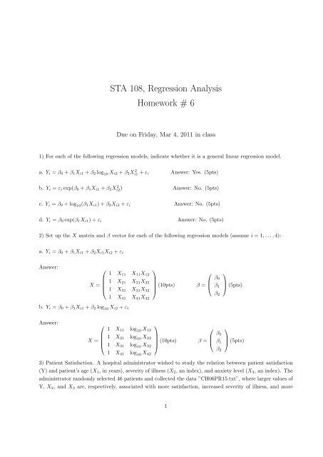
1) For each of the following regression models, indicate whether it is a general linear regression model.
a. Yi = β0 + β1Xi1 + β2 log 10 Xi2 + β3X 2 i1
+ εi
Answer:
Yes. (5pts)
b. Yi = εi exp(β0 + β1Xi1 + β2X 2 i2 ) Answer: No. (5pts)
c. Yi = β0 + log 10(β1Xi1) + β2Xi2 + εi
d. Yi = β0 exp(β1Xi1) + εi
Answer: No. (5pts)
Answer: No. (5pts)
2) Set up the X matrix and β vector for each of the following regression models (assume i = 1, . . . , 4):
a. Yi = β0 + β1Xi1 + β2Xi1Xi2 + εi
Answer:
⎛
⎜
X = ⎜
⎝
b. Yi = β0 + β1Xi1 + β2 log 10 Xi2 + εi
Answer:
⎛
⎜
X = ⎜
⎝
1 X11 X11X12
1 X21 X21X22
1 X31 X31X32
1 X41 X41X42
1 X11 log 10 X12
1 X21 log 10 X22
1 X31 log 10 X32
1 X41 log 10 X42
⎞
⎛
⎟
⎜
⎟ (10pts) β = ⎝
⎠
⎞
⎛
⎟
⎜
⎟ (10pts) β = ⎝
⎠
β0
β1
β2
β0
β1
β2
⎞
⎟
⎠ (5pts)
⎞
⎟
⎠ (5pts)
3) Patient Satisfaction. A hospital administrator wished to study the relation between patient satisfaction
(Y) and patient’s age (X1, in years), severity of illness (X2, an index), and anxiety level (X3, an index). The
administrator randomly selected 46 patients and collected the data ”CH06PR15.txt”, where larger values of
Y, X2, and X3 are, respectively, associated with more satisfaction, increased severity of illness, and more
1

anxiety.
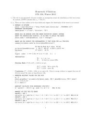
a. Fit regression model for three predictor variables to the data and state the estimated regression function.
How is b2 interpreted here?
Answer: The estimated regression function is ˆ Y = 158.4913 − 1.1416X1 − 0.4420X2 − 13.4702X3 (10pts)
b2 is an estimate of the change in the mean response per unit increase in X2 when X1 and X3 are held
constant. (10pts)
b. Plot the residuals against ˆ Y , and each of the predictor variables on separate graphs(20pts). Interpret
your plots and summarize your findings (10pts).
residuals
residuals
−15 −5 0 5 10
−15 −5 0 5 10
(a)Residual Plot against Fitted Value
40 50 60 70 80 90
fitted values
(c)Residual Plot against X2
45 50 55 60
severity of illness
residuals
residuals
−15 −5 0 5 10
−15 −5 0 5 10
Figure 1: residual plot
(b)Residual Plot against X1
25 30 35 40 45 50 55
patient’s age
(d)Residual Plot against X3
1.8 2.0 2.2 2.4 2.6 2.8
anxiety level
Plot(a) is the residual e against the fitted values ˆ Y , it does not suggest any systematic deviations from the
response plane, nor that the variance of the error terms varies with the level of ˆ Y . Plots of the residuals e
against X1 and X2 in (b), (c) and (d), are entirely consistent with the conclusions of good fit by the response
function and constant variance of the error terms.(10pts)
2