STA 106: Midterm – Solutions - Statistics

STA 106: Midterm – Solutions
February 17, 2012
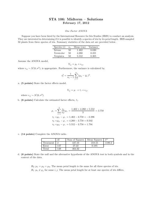
One Factor ANOVA
Suppose you have been hired by the International Resource for Iris Studies (IRIS) to conduct an analysis.
They are interested in determining if it is possible to identify a species of iris by its petal length. IRIS sampled
50 plants from three species of iris. Summary statistics of the data set are provided below.
Assume the ANOVA model,
Species (i) ni Mean (cm) Variance
Setosa 50 1.462 0.030
Versicolor 50 4.260 0.221
Verginica 50 5.552 0.305
Yij = µi + ɛij,
where ɛij ∼ N (0, σ 2 ), is appropriate. Furthermore, the variance is calculated by,
a. (5 points) State the factor effects model.
where ɛij ∼ N (0, σ 2 ).
s 2 i = 1
ni − 1
ni
(yij − ¯yi·) 2 .
j=1
Yij = µ·· + τi + ɛij,
b. (6 points) Calculate the estimated factor effects, ˆτi.
µ·· =
3
ni
nT
i=1
c. (14 points) Complete the ANOVA table.
µi· =
1.462 + 4.260 + 5.552
3
τ1 =µ1· − µ·· = 1.462 − 3.758 = −2.296
τ2 =µ2· − µ·· = 4.260 − 3.758 = 0.502
τ3 =µ3· − µ·· = 5.552 − 3.758 = 1.794
= 3.758
df Sum of Squares Mean Squares F ∗
Treatment 2 437.10 218.55 1180.2
Error 147 27.22 0.185
Total 149 464.32
d. (6 points) State the null and the alternative hypothesis of the ANOVA test in both symbols and in the
context of the data.
H0 :µ1 = µ2 = µ3. The mean petal length is the same for all three species of iris.
H1 :µi = µj for some i, j. The mean petal length for at least one species of iris differs.

e. (5 points) Assume the significance level of the test is α = 5%. Find the critical value for the test statistic.
Fcrit(.95; 2, 147) = 3.058
f. (5 points) Based on the ANOVA table and critical value, what conclusion can you draw about the petal
length of the three iris species?
I would reject the null hypothesis. The mean petal length for at least one species of iris differs.
g. (8 points) If you were to conduct pairwise comparisons for the three species of iris, which method, Tukey,
Scheffe, or Bonferroni, would be most appropriate? Explain and justify your answer numerically (You do
not need to calculate the intervals).
T = 1
√ 2 q(.95; 3, 150 − 3) = 3.348
√ 2 = 2.367
S = (3 − 1)F (.95; 3 − 1, 150 − 3) = 2(3.058) = 2.473
B =t(1 − .05
, 150 − 3) = 2.352
2(3)
Here, Bonferroni is best as it has the smallest statistic, so it will yield the most precise confidence intervals.
h. (10 points) Now suppose the researchers at IRIS, prior to seeing the data, suspected that the versicolor
and verginica species would be very similar, but wanted to know if these species differed from setosa.
Propose a contrast to test this and calculate the confidence interval for the contrast (α = .10). What can
you conclude from this interval?
To test if versicolor and verginica are different than setosa, we can use the contrast L = 2 × µsetosa −
µversicolor − µverginica. Any constant times this contrast would work as well.
ˆL = 2ˆµ1 − ˆµ2 − ˆµ3 = −6.888
sˆ
L = MSE c2
i 0.185
= (4 + 1 + 1) = 0.149
ni 50
t(1 − α/2, nT − r) = t(.95, 147) = 1.655
CI : −6.888 ± 1.655(0.149) = (−7.135, −6.641)
This interval does not include zero. Thus, there is significant evidence to suggest that the mean petal
length of versicolor and verginica differs from that of setosa.
i. (5 points) Judging by the summary statistics given from the data, does it appear that any assumptions
of the ANOVA model are violated? If so, which assumption?
It appears that the assumption of equal variance for all groups may be violoated. The setosa group has
a much smaller variance than the other two.
j. (10 points) If assumptions of the ANOVA model were violated suggest another method that could be
used to test the hypotheses given in part d. List and describe the steps and calculations required to
conduct the test you recommended (do not actually carry out the test).
If the distributional assumptions of the ANOVA model are violated we could use the nonparametric F
test. The test can be done in the following steps:
1. Replace each observation with its corresponding rank.

2. Compute,
3. Compute,
4. Calculate the test statistic,
ni(
MST R =
¯ Ri· − ¯ R··) 2
.
r − 1
(Rij −
MSE =
¯ Ri·) 2
nT − r
F ∗ = MST R/MSE
5. Compare the test statistic to its probability distribution under the null hypothesis and draw a conclusion.
If F ∗ ≤ F (1 − α; r − 1, nT − r), conclude H0
If F ∗ > F (1 − α; r − 1, nT − r), conclude H1
Two Factor ANOVA
Consider the two-factor model summarized by factor combination means, µij in the table below.
Factor 2
Factor 1 j = 1 j = 2 j = 3
i = 1 96 112 80
i = 2 116 100 132
a. (5 points) Below is an interaction plot of the data. Describe any interaction or main effects visible in
the plot.

As the lines are not close to parallel there is evidence of a strong interaction effect. It can be seen that
if you average over Factor 1 you will obtain similar values at both levels of Factor 2, but this is not true
for averaging over Factor 1. This indicates there may be a main effect for Factor 1 and no main effect for
Factor 2.
b. (6 points) Calculate the main effects for factor 1, αi, and the main effects for factor 2, βj.
96 + 112 + 80 + 116 + 100 + 132
µ·· =
96 + 112 + 80
α1 = − 106 = −10
3
116 + 100 + 132
α2 = = 10
3
96 + 116
β1 = − 106 = 0
2
112 + 100
β2 = − 106 = 0
β3 =
2
80 + 132
2
6
− 106 = 0
= 106
c. (10 points) Let the sample size for each factor combination be n = 5 and let σ = 3. Compute E{MSE}
and E{MSAB}.
E{MSE} =σ 2 = 3 2 = 9
E{MSAB} =σ 2
(µij − µi· − µ·j + µ··)
+ n
2
(a − 1)(b − 1)
=9 + 5
(µij − µi· + (106 − 106))
2
2
=9 + 5
2 (02 + 16 2 + (−16) 2 + 0 2 + (−16) 2 + 16 2 )
=9 + 5
2 4(162 ) = 2569
d. (5 points) Is E{MSAB} significantly larger than E{MSE}? What is the significance of this?
Yes, E{MSAB} is much larger than E{MSE}. This indicates that there is a very significant interaction
effect in the model given by the means above.