- Page 1: Deutsche Geophysikalische Gesellsch
- Page 5 and 6: Vorwort Das Kolloquium Elektromagne
- Page 7 and 8: Ι Ι Ι Teilnehmerverzeichnis Bara
- Page 9 and 10: Schwarz Gerhard Geological Survey o
- Page 11 and 12: 01. 1962 Kassel 02. 1963 Salzgitter
- Page 14 and 15: Meine „Inauguration“ fand auf d
- Page 16 and 17: „An Geräten gab‘s anfangs nur
- Page 18 and 19: Sicherungen Einstellen der Galvanom
- Page 20 and 21: „In unserem Kreis sind Mensch und
- Page 22 and 23: Herr Andersohn, der Schöpfer der A
- Page 24 and 25: Das Kolloquium sollte, wie es das l
- Page 26 and 27: Es entstand die Frage, ob wir nach
- Page 30 and 31: Es fällt leichter, sich mit dem Er
- Page 32 and 33: Urerfahrungen des Menschen Ich glau
- Page 34 and 35: Kapitel „Ungelöste Probleme“:
- Page 36 and 37: Es bleibt immer noch zu viel stehen
- Page 39 and 40: 1D interpretation of electromagneti
- Page 41 and 42: ( 0) ∂Fn ( 0) yn − Fn ( xm ; d'
- Page 43 and 44: exactly the same way. When only pha
- Page 45 and 46: data errors and the often extreme c
- Page 47: with few layers are considered. Ide
- Page 50 and 51: Proceeding as before, now with deri
- Page 52 and 53:
with = J or . z d z J z G z G ′ )
- Page 54 and 55:
A visual display of this balanced i
- Page 56 and 57:
as outlined in Subsection 4.6 and 4
- Page 58 and 59:
egularisation, leading to a more st
- Page 60 and 61:
of the trade-off parameter w has be
- Page 62 and 63:
shown in Fig. 7. The curve to the l
- Page 64 and 65:
References Berdichevsky, M.N. & V.I
- Page 66 and 67:
−1 + Ψ tanh { exp{ 2 ′ m U m
- Page 68 and 69:
the solution coefficients v kn rema
- Page 70:
1 ∑hk nbnn = − [ λ k + ( 1−
- Page 73 and 74:
In the case of a layered mantle it
- Page 75 and 76:
The present more elementary approac
- Page 77 and 78:
the time constants are reversely gi
- Page 79 and 80:
3.2. Diffusion pattern of radial an
- Page 81 and 82:
Figure 4: Degree ℓ = 1, impulse d
- Page 83 and 84:
The recursion starts with ψℓ0(r)
- Page 85 and 86:
3.4. Relationship between τℓ, σ
- Page 87 and 88:
Mercer’s theorem (Courant & Hilbe
- Page 89 and 90:
Moreover let Θ(x) with Θ(x)+Θ(
- Page 91 and 92:
METHOD OF HORIZONTAL MAGNETOVARIATI
- Page 93 and 94:
2. Estimation of the horizontal mag
- Page 95 and 96:
Figure 4. Pseudo sections of the ho
- Page 97 and 98:
Figure 5. Pseudo sections of rotati
- Page 99 and 100:
5. Two-dimensional inversion of the
- Page 101 and 102:
Figure 10a. M xx data inversion at
- Page 103 and 104:
Varentsov, Iv.M., 2005b. Arrays of
- Page 105 and 106:
Figure 1. The EMTESZ-Pomerania arra
- Page 107 and 108:
0 the variability criterion: M-tens
- Page 109 and 110:
sites ranging from 3 to 6 at distan
- Page 111 and 112:
sufficiently “clean” responses.
- Page 114:
ailways and other dominant industri
- Page 117 and 118:
Kanonische Kohärenzen - Indikator
- Page 119 and 120:
4 Beispiele Parkfield 2005 Im Früh
- Page 121 and 122:
∗ †
- Page 123 and 124:
o
- Page 125 and 126:
• •
- Page 127 and 128:
ties of their estimates is of essen
- Page 129 and 130:
where θ0 is used to adjust limits
- Page 131 and 132:
RMS squared Twist (deg) 10 1 0.1 0.
- Page 133 and 134:
Site True twist True shear MNJ twis
- Page 135 and 136:
References Bahr, K., 1988. Interpre
- Page 137 and 138:
ihre Elemente durch Hochkommata ind
- Page 139 and 140:
vernachlässigen ist. Dieser Grenzw
- Page 141 and 142:
M´ xx T´ 21 1500 1000 500 0 −50
- Page 143 and 144:
T´ 21 M´ xx 0.4 0.2 0 −0.2 −0
- Page 145 and 146:
inversion model parameters. The per
- Page 147:
There remains the open problem to s
- Page 150 and 151:
Figure 4: Fitting between observed
- Page 152 and 153:
simulation is done applying an adap
- Page 154 and 155:
Let y be the strike direction of a
- Page 156:
ρ a in Ω⋅ m φ in degrees 10 3
- Page 159 and 160:
7 Topography Fig. 7: Real (left) an
- Page 161:
Fig. 11: Real part of current densi
- Page 164 and 165:
2. An der Grenze zwischen zwei Gebi
- Page 166 and 167:
Abbildung 1: Ausschnitt eines Hexae
- Page 168 and 169:
Abbildung 4: Oktant einer Kugel. Ve
- Page 171 and 172:
3D-TEM-Simulation für axialsymmetr
- Page 173:
4 Transformation der Felder in den
- Page 176:
E φ in V/m E φ in V/m 10 −6 10
- Page 179 and 180:
• coincident-loop configuration,
- Page 181 and 182:
generally
- Page 183 and 184:
fictitious anomalies are also intro
- Page 185 and 186:
(2001). The studies of Goldman et a
- Page 187 and 188:
1 1 1
- Page 189 and 190:
X = x i | i = 1, 2, 3
- Page 191 and 192:
g R g ijk
- Page 193 and 194:
Ωm m m
- Page 195 and 196:
∂σ = ∂ m −1 = −m −2 ∂
- Page 197 and 198:
Der Reflexionsfaktor D beschreibt d
- Page 199 and 200:
Rotationsellipsoide Eine komplexere
- Page 201 and 202:
Dipolmomente der der ideal leitende
- Page 204 and 205:
Die Spulen im Gerät bestehen in Wi
- Page 206 and 207:
Abbildung 10: Ortsphasenkurven übe
- Page 208 and 209:
mit der kommerziellen Software FEML
- Page 210 and 211:
Gehäuse und eine Sprengstofffüllu
- Page 212 and 213:
Abb. 10: Profil über eine Kugel un
- Page 214 and 215:
für Elektrotechnik der Universitä
- Page 216 and 217:
sind die genaue Anzahl der Wicklung
- Page 219 and 220:
Inversion von Felddaten Im Rahmen d
- Page 221 and 222:
Abbildung 16: Anpassung der gewicht
- Page 223 and 224:
Resolution and depth of investigati
- Page 225 and 226:
R m i 0.06 0.05 0.04 0.03 0.02 0.01
- Page 227 and 228:
λ i 10 5 10 0 10 −5 10 −10 sin
- Page 229 and 230:
Zeitreihenauswertung von NMR Messun
- Page 231 and 232:
• Ein Störsignal am Ort der Basi
- Page 233 and 234:
B Y B X Reference Loops Receiver AD
- Page 235 and 236:
Amplitude /V Amplitude /V Amplitude
- Page 237 and 238:
Diskussion und Ausblick Einerseits
- Page 239 and 240:
Topography Parameter mesh Primary f
- Page 241 and 242:
sion result is shown in form of two
- Page 243 and 244:
Sophisticated constraints Underwate
- Page 245 and 246:
Ellis, R. G. and Oldenburg, D. W. (
- Page 247 and 248:
2. Frequenzabhängigkeiten B n z wi
- Page 249 and 250:
durch die magnetische Aktivität be
- Page 251 and 252:
Frequenzverhältnis abgeleiteten An
- Page 253 and 254:
273
- Page 255 and 256:
275
- Page 257 and 258:
mantle anisotropy same background c
- Page 259 and 260:
imately 160km. The first 10km thick
- Page 261 and 262:
Uniform Deflection of Induction Vec
- Page 263 and 264:
can plates. It may be speculated th
- Page 265 and 266:
Fig. 4a: 2-D anisotropic model yiel
- Page 267 and 268:
(e.g., Lanalhue Fault) would be nec
- Page 269 and 270:
deepening Moho from 32-35 km in the
- Page 271 and 272:
Fig. 4 2-D Model calculated with th
- Page 273 and 274:
36.2°N 36.0°N 35.8°N SAFOD Parkf
- Page 275 and 276:
¥§¦ App. Resistivity (ohm−m) P
- Page 277 and 278:
¢¡¤£¥¡§¦¨¡¤©¡¤ ¢ ¢
- Page 279 and 280:
0311 0310 0308 0309 0307 0306 0021
- Page 281 and 282:
Outlook After adopting the finite e
- Page 283 and 284:
0 5 10 15 20 25 A 30 10 N 20 30 40
- Page 285 and 286:
Figure 5: With a simple 2D model we
- Page 287 and 288:
An Amphibious Magnetotelluric Exper
- Page 289 and 290:
Fig. 2: Deployment of the HEFMAG se
- Page 291 and 292:
Transfer functions Analysis of the
- Page 293 and 294:
Fig. 7b: Induction vectors for 3277
- Page 295 and 296:
Untersuchungen der Bremerhaven-Cuxh
- Page 297 and 298:
Hubschrauber-Elektromagnetik (HEM)
- Page 299 and 300:
Messgebiet Wanhöden Die Bremerhave
- Page 301 and 302:
Depth [m] 0 20 40 60 80 100 120 140
- Page 303 and 304:
Um die Inversionsergebnisse richtig
- Page 305 and 306:
Geoelektrische Tiefensondierungen
- Page 307 and 308:
Faustformel kann hier eine Eindring
- Page 309 and 310:
Beim gezeigten Modell treten zwei d
- Page 311 and 312:
Einleitung Messung der TEM-Antwort
- Page 313 and 314:
Dipole nimmt mit der Größe des Ko
- Page 315 and 316:
Induzierte Spannung (normiert) V/A*
- Page 317 and 318:
Tiefe in m 0 2 4 6 8 10 12 14 16 St
- Page 319 and 320:
Investigation of the Groundwater Re
- Page 321 and 322:
The Eiseb Graben was exclusively se
- Page 323 and 324:
Figure 3: TEM sounding and 1d inver
- Page 325 and 326:
that performed by INTERCONSULT (199
- Page 327 and 328:
old age and was recharged under dif
- Page 329 and 330:
KLOCK, H. (2001): Hydrogeology of t
- Page 331 and 332:
Figure 1: Survey area on the Cascad
- Page 333 and 334:
Figure 4: Data along profile 4 as l
- Page 335 and 336:
Vent Field The vent field is charac
- Page 337 and 338:
Recent drilling results at IODP sit
- Page 339 and 340:
sounding: Hydrate without a BSR? Ge
- Page 341 and 342:
Abb. 1: Schematische Darstellung de
- Page 343 and 344:
Abb. 7: Vergleich der FDR- und Geor
- Page 345 and 346:
Applicability of RMT, VES and Dual
- Page 347 and 348:
Profile 5 Profile 6 Profile 3 Profi
- Page 349 and 350:
According to the latter, one has to
- Page 351 and 352:
Figure 6: HLEM raw data: Iphase and
- Page 353 and 354:
6WRQHOH\ ZDYH LQGXFHG HOHFWURNLQHWL
- Page 355 and 356:
1991). I n this case wave propagati
- Page 357 and 358:
to m easure the density, consists o
- Page 359 and 360:
7DEOH 3K\VLFDO SURSHUWLHV RI WZR VD
- Page 361 and 362:
Using a finite elem ent code (Pain
- Page 363 and 364:
experim entally that NEF is a funct
- Page 365 and 366:
Umbau von MAGSON-Magnetometern und
- Page 367 and 368:
Abb. 3 Elektronik in Operation Link
- Page 369 and 370:
Die magn. Flussdichte in Richtung d
- Page 371 and 372:
a) b) * Ursache EDL, Speichervorgan
- Page 373 and 374:
(a) (b) Abbildung 1: a) Prototyp ei
- Page 375 and 376:
γ und Gleichung (8) mit einer vekt
- Page 377 and 378:
Sonde Bewegungsrichtung der horizon
- Page 379 and 380:
] m [ z Sondenelektroden: TX RX k r
- Page 381 and 382:
Geophysikalische Erkundung des Kohl
- Page 383 and 384:
Die Vertikalsektion des spezifische
- Page 385 and 386:
Abb. 5: Vertikalsektion des spezifi
- Page 387 and 388:
Abb. 8: Anomalien des Magnetfeldes
- Page 389 and 390:
Gleichstromgeoelektrische Untersuch
- Page 391 and 392:
Abb. 1: Lage der Profile und Nummer
- Page 393 and 394:
Der spezifische Widerstand von Salz
- Page 395 and 396:
Maximum-Norm-Abweichung (L ∞ -Nor
- Page 397 and 398:
Abb. 4: Sondierungskurve (ρs -Kurv
- Page 399 and 400:
Vergleich von geoelektrischen und H
- Page 401 and 402:
Fig. 7: Comparison of HEM inversion
- Page 403 and 404:
von 21% und eine lsq-Abweichung von
- Page 405:
A. & STOLL, J. (Hrsg.): Protokoll