mechanical behaviour of unsaturated aggregated soils - EPFL

Mechanical Behaviour
of unsaturated aggregated soils
THÈSE N O 4011 (2008)
PRÉSENTÉE LE 25 jANVIER 2008
À LA FACULTÉ DE L'ENVIRONNEMENT NATUREL, ARCHITECTURAL ET CONSTRUIT
LABORATOIRE DE MÉCANIQUE DES SOLS
PROGRAMME DOCTORAL EN MÉCANIQUE
ÉCOLE POLYTECHNIQUE FÉDÉRALE DE LAUSANNE
POUR L'OBTENTION DU GRADE DE DOCTEUR ÈS SCIENCES
PAR
Azad KOLIjI
M.Sc. in civil engineering, Iran University of science and technology, Tehran, Iran
et de nationalité iranienne
acceptée sur proposition du jury:
Prof. L. Laloui, président du jury
Prof. L. Vulliet, directeur de thèse
Prof. R. Charlier, rapporteur
Prof. P. Delage, rapporteur
Prof. H. Flühler, rapporteur
Suisse
2008

To my grandmother Daya & my aunt Mina

Contents
Acknowledgments vii
Abstract ix
Résumé xi
List of Symbols xiii
1 Introduction 1
1.1 From saturated homogeneous to unsaturated structured soil . . 1
1.2 Objectives . . . . . . . . . . . . . . . . . . . . . . . . . . . . . . 2
1.3 Outline of the thesis . . . . . . . . . . . . . . . . . . . . . . . . 3
2 Background and problem addressing 5
2.1 Essential concepts . . . . . . . . . . . . . . . . . . . . . . . . . . 5
2.1.1 Soil structure . . . . . . . . . . . . . . . . . . . . . . . . 5
2.1.2 Pore fluid . . . . . . . . . . . . . . . . . . . . . . . . . . 7
2.1.2.1 Pore water potential . . . . . . . . . . . . . . . 7
2.1.2.2 Suction in unsaturated soils . . . . . . . . . . . 9
2.1.3 Multi-scale heterogeneity . . . . . . . . . . . . . . . . . . 9
2.1.4 Structured soil . . . . . . . . . . . . . . . . . . . . . . . 10
2.1.4.1 Natural bonded soils . . . . . . . . . . . . . . . 10
2.1.4.2 Aggregated soils . . . . . . . . . . . . . . . . . 11
2.1.5 Concept of double porosity . . . . . . . . . . . . . . . . . 13
2.2 Partial saturation effects . . . . . . . . . . . . . . . . . . . . . . 15
2.2.1 Water retention characteristics . . . . . . . . . . . . . . . 15
2.2.2 Capillary effects . . . . . . . . . . . . . . . . . . . . . . . 17
2.3 Fabric effects in unsaturated soils . . . . . . . . . . . . . . . . . 18
2.3.1 Influence on water retention characteristics . . . . . . . . 18
2.3.2 Collapsible behavior . . . . . . . . . . . . . . . . . . . . 20
2.4 Inter-particle bonding effects . . . . . . . . . . . . . . . . . . . . 22
2.4.1 Pre-yield behavior . . . . . . . . . . . . . . . . . . . . . 22
2.4.2 Yield limit . . . . . . . . . . . . . . . . . . . . . . . . . . 22
2.4.3 Yielding behavior . . . . . . . . . . . . . . . . . . . . . . 24
2.4.4 Combined effects of bonding and partial saturation . . . 27
2.5 Study of soil structure . . . . . . . . . . . . . . . . . . . . . . . 28
2.5.1 Experimental methods for soil fabric study . . . . . . . . 28
i

2.5.2 Fabric evolution . . . . . . . . . . . . . . . . . . . . . . . 29
2.6 Constitutive modeling . . . . . . . . . . . . . . . . . . . . . . . 31
2.6.1 Effective stress . . . . . . . . . . . . . . . . . . . . . . . 31
2.6.2 Constitutive modeling of unsaturated soils . . . . . . . . 35
2.6.2.1 Modeling approaches . . . . . . . . . . . . . . . 35
2.6.2.2 Double structure model for unsaturated soils . . 37
2.6.3 Constitutive modeling of natural bonded soils . . . . . . 39
2.6.3.1 Modelling approaches . . . . . . . . . . . . . . 39
2.6.3.2 Representative models for saturated bonded soil 40
2.6.3.3 Extension of models for unsaturated bonded soil 45
2.7 Summary and anticipated contribution . . . . . . . . . . . . . . 47
3 Hydro-mechanical formulation for double porous soil 49
3.1 Theoretical framework . . . . . . . . . . . . . . . . . . . . . . . 49
3.1.1 Thermodynamic approaches . . . . . . . . . . . . . . . . 49
3.1.2 General formulation . . . . . . . . . . . . . . . . . . . . 53
3.2 Mixture model of soil with double porosity . . . . . . . . . . . . 57
3.2.1 Double mixture approach . . . . . . . . . . . . . . . . . 57
3.2.2 Mass balance . . . . . . . . . . . . . . . . . . . . . . . . 61
3.2.2.1 Solid mass balance . . . . . . . . . . . . . . . . 61
3.2.2.2 Fluid mass balance . . . . . . . . . . . . . . . . 61
3.2.3 Linear momentum balance . . . . . . . . . . . . . . . . . 61
3.3 Constitutive equations . . . . . . . . . . . . . . . . . . . . . . . 64
3.3.1 Stress tensor . . . . . . . . . . . . . . . . . . . . . . . . . 64
3.3.1.1 Stress tensor in fluids . . . . . . . . . . . . . . 64
3.3.1.2 Stress tensor in solid . . . . . . . . . . . . . . . 64
3.3.1.3 Total stress tensors . . . . . . . . . . . . . . . . 66
3.3.1.4 Total fluid pressure and total suction . . . . . . 66
3.3.1.5 Effective stress . . . . . . . . . . . . . . . . . . 67
3.3.2 Mechanical constitutive equation . . . . . . . . . . . . . 68
3.3.3 Equation of state for fluid . . . . . . . . . . . . . . . . . 69
3.3.4 Fluid flow . . . . . . . . . . . . . . . . . . . . . . . . . . 69
3.3.5 Liquid retention . . . . . . . . . . . . . . . . . . . . . . . 71
3.3.6 Fluid mass transfer between mixtures . . . . . . . . . . . 71
3.4 General field equations . . . . . . . . . . . . . . . . . . . . . . . 72
3.5 Summary of field equations . . . . . . . . . . . . . . . . . . . . 74
4 Experimental characterization of macroscopic behavior 77
4.1 Objectives and methods . . . . . . . . . . . . . . . . . . . . . . 77
4.1.1 Objectives and experimental approaches . . . . . . . . . 77
4.1.2 Existing suction control methods . . . . . . . . . . . . . 78
4.1.2.1 Axis translation technique . . . . . . . . . . . . 78
4.1.2.2 Vapor equilibrium method . . . . . . . . . . . . 80
4.1.2.3 Osmotic method . . . . . . . . . . . . . . . . . 82
4.1.3 Choice of methods and equipments . . . . . . . . . . . . 85
4.2 Development of a new osmotic oedometer . . . . . . . . . . . . . 86
ii

4.2.1 Osmotic oedometer components . . . . . . . . . . . . . . 86
4.2.1.1 Oedometer cell and mechanical loading . . . . . 87
4.2.1.2 Semi-permeable membrane and PEG solution . 88
4.2.1.3 Tubing, pump and reservoir . . . . . . . . . . . 90
4.2.1.4 Electronic Balance . . . . . . . . . . . . . . . . 90
4.2.2 Control and callibration of the cell . . . . . . . . . . . . 90
4.2.3 Suction control and PEG concentration . . . . . . . . . . 92
4.2.4 Water exchange measurements and calibration . . . . . . 96
4.2.5 Hints on testing procedure . . . . . . . . . . . . . . . . . 98
4.3 Material and program . . . . . . . . . . . . . . . . . . . . . . . 99
4.3.1 Material characteristics . . . . . . . . . . . . . . . . . . . 99
4.3.2 Aggregate preparation . . . . . . . . . . . . . . . . . . . 99
4.3.3 Experimental program . . . . . . . . . . . . . . . . . . . 103
4.4 Dry and saturated behavior . . . . . . . . . . . . . . . . . . . . 104
4.4.1 Description of the tests . . . . . . . . . . . . . . . . . . . 104
4.4.2 Results of dry tests . . . . . . . . . . . . . . . . . . . . . 107
4.4.3 Results of saturated tests . . . . . . . . . . . . . . . . . . 111
4.4.4 Results of soaking tests . . . . . . . . . . . . . . . . . . . 112
4.4.4.1 Simple soaking of aggregated samples . . . . . . 112
4.4.4.2 Oedometric soaking of aggregated samples . . . 112
4.5 Unsaturated behavior . . . . . . . . . . . . . . . . . . . . . . . . 114
4.5.1 Description of the tests . . . . . . . . . . . . . . . . . . . 114
4.5.2 Osmotic oedometer tests on reconstituted soil . . . . . . 116
4.5.3 Osmotic oedometer tests on aggregated soil . . . . . . . 123
4.6 Comparison and discussion of results . . . . . . . . . . . . . . . 130
4.6.1 Aggregated versus reconstituted samples . . . . . . . . . 130
4.6.2 Suction effects . . . . . . . . . . . . . . . . . . . . . . . . 133
4.7 Summary of results . . . . . . . . . . . . . . . . . . . . . . . . . 139
5 Experimental study of soil structure 141
5.1 Objectives and methods . . . . . . . . . . . . . . . . . . . . . . 141
5.1.1 Objectives and experimental approaches . . . . . . . . . 141
5.1.2 Mercury intrusion porosimetry . . . . . . . . . . . . . . . 142
5.1.3 Environmental scanning electron microscopy . . . . . . . 144
5.1.4 Neutron radiography and tomography . . . . . . . . . . . 145
5.2 Fabric evaluation using MIP and ESEM . . . . . . . . . . . . . 146
5.2.1 Sample preparation . . . . . . . . . . . . . . . . . . . . . 146
5.2.2 Description of MIP tests . . . . . . . . . . . . . . . . . . 147
5.2.3 MIP Results . . . . . . . . . . . . . . . . . . . . . . . . . 148
5.2.3.1 Porosity of specimens . . . . . . . . . . . . . . 148
5.2.3.2 Unsaturated aggregated samples . . . . . . . . 149
5.2.3.3 Aggregated samples after soaking . . . . . . . . 152
5.2.3.4 Reconstituted samples . . . . . . . . . . . . . . 153
5.2.3.5 Comparison of results . . . . . . . . . . . . . . 154
5.2.4 Description of ESEM observations . . . . . . . . . . . . . 156
5.2.5 ESEM results . . . . . . . . . . . . . . . . . . . . . . . . 156
iii

5.3 Tomography evaluation of soil structure under mechanical loading 165
5.3.1 Material and method . . . . . . . . . . . . . . . . . . . . 165
5.3.2 Experimental set up and procedure . . . . . . . . . . . . 165
5.3.3 Processing of raw image data . . . . . . . . . . . . . . . 168
5.3.4 Macroscopic results . . . . . . . . . . . . . . . . . . . . . 171
5.3.5 Characterization of soil structure evolution . . . . . . . . 172
5.3.6 Evaluation of structure degradation mechanisms . . . . . 175
5.4 Tomography evaluation of soil structure under suction variation 179
5.4.1 Material and method . . . . . . . . . . . . . . . . . . . . 179
5.4.2 Experimental set up and procedure . . . . . . . . . . . . 179
5.4.3 Processing of raw image data . . . . . . . . . . . . . . . 180
5.4.3.1 Radiography data . . . . . . . . . . . . . . . . 180
5.4.3.2 Tomography data . . . . . . . . . . . . . . . . . 181
5.4.4 Suction-induced volume change of aggregates . . . . . . . 184
5.5 Summary of results . . . . . . . . . . . . . . . . . . . . . . . . . 185
6 Mechanical constitutive model 187
6.1 Constitutive framework . . . . . . . . . . . . . . . . . . . . . . . 187
6.1.1 Stress framework . . . . . . . . . . . . . . . . . . . . . . 187
6.1.2 Critical state line for unsaturated aggregated soils . . . . 188
6.1.3 Fundamental formulation . . . . . . . . . . . . . . . . . . 190
6.2 Requirements of the new model . . . . . . . . . . . . . . . . . . 193
6.2.1 Features to be addressed . . . . . . . . . . . . . . . . . . 193
6.2.2 Pre-yield and elastic behavior . . . . . . . . . . . . . . . 196
6.2.3 Yielding and apparent preconsolidation pressure . . . . . 197
6.2.4 Post-yield behavior and hardening . . . . . . . . . . . . . 198
6.2.5 Plastic multiplier and plastic potential . . . . . . . . . . 199
6.3 Soil structure parameters . . . . . . . . . . . . . . . . . . . . . . 200
6.3.1 Degree of soil structure . . . . . . . . . . . . . . . . . . . 200
6.3.2 Structure degradation . . . . . . . . . . . . . . . . . . . 203
6.3.3 Influence of suction on structure parameters . . . . . . . 204
6.3.4 Determination procedure . . . . . . . . . . . . . . . . . . 206
6.4 Model formulation ACMEG-2S . . . . . . . . . . . . . . . . . . 208
6.4.1 Introduction to the model developments . . . . . . . . . 208
6.4.2 Elastic components of the model . . . . . . . . . . . . . 209
6.4.3 Yield criteria . . . . . . . . . . . . . . . . . . . . . . . . 211
6.4.4 Apparent preconsolidation pressure and hardening . . . . 214
6.4.5 Plastic potential and plastic multipliers . . . . . . . . . . 219
6.4.6 General stress-strain relationship . . . . . . . . . . . . . 222
6.4.7 Variation of degree of saturation . . . . . . . . . . . . . . 225
6.5 Assessment of model parameters . . . . . . . . . . . . . . . . . . 229
6.5.1 Model parameters . . . . . . . . . . . . . . . . . . . . . . 229
6.5.2 Parameter determination for Bioley silt . . . . . . . . . . 231
6.6 Simulation and validation . . . . . . . . . . . . . . . . . . . . . 236
6.6.1 Numerical integration of the constitutive equations . . . 236
6.6.2 Typical numerical response . . . . . . . . . . . . . . . . . 236
iv

6.6.2.1 Isotropic consolidation . . . . . . . . . . . . . . 236
6.6.2.2 Conventional triaxial compression (CTC) . . . 239
6.6.3 Simulation of the oedometer tests . . . . . . . . . . . . . 240
6.6.3.1 Saturated and dry samples . . . . . . . . . . . . 240
6.6.3.2 Unsaturated reconstituted samples . . . . . . . 242
6.6.3.3 Unsaturated aggregated samples . . . . . . . . 245
6.6.4 Assessment of model for saturated bonded soils . . . . . 250
6.7 Conclusion . . . . . . . . . . . . . . . . . . . . . . . . . . . . . . 255
7 Conclusions and recommendations for future research 257
7.1 Conclusions . . . . . . . . . . . . . . . . . . . . . . . . . . . . . 257
7.1.1 Governing equations . . . . . . . . . . . . . . . . . . . . 258
7.1.2 Experimental approach . . . . . . . . . . . . . . . . . . . 259
7.1.2.1 Methods . . . . . . . . . . . . . . . . . . . . . . 259
7.1.2.2 Experimental results . . . . . . . . . . . . . . . 260
7.1.3 Constitutive modeling . . . . . . . . . . . . . . . . . . . 263
7.2 Outlook for future works . . . . . . . . . . . . . . . . . . . . . . 264
References 267
A Control tests for the new osmotic oedometer cell 287
B Supplementary experimental results 291
C Modeling suction effects on the fabric of an aggregated soil 295
v

Acknowledgments
This thesis is the result of four years of work whereby I have been accompanied
and supported by many people. I would like to thank the diverse group of
individuals who supported my work, influenced my thoughts and participated
in this study. Without each one of them, this project simply would not have
been possible.
Foremost, I would like to express my sincere gratitude to my thesis supervisor,
Prof. Laurent Vulliet, for his support and mentorship through this study,
and for his constant confidence in my abilities. I admire his affirmative professional
attitude, and his efficient mindful approach to simplify complexities.
I would like to acknowledge my debt to Prof. Lyesse Laloui for his highly
responsive supports over the duration of this work. His contribution is apparent
all over my dissertation. Beyond all his contribution to my work, I would like to
thank Prof. Laloui for his limitless facility to initiate exploration in the world
of scholarship and for opening my eyes to the elegance of “scholarly life”.
I would like to thank Peter Vontobel, Eberhard Lehmann and, René Hassanein
of the Neutron Imaging group of PSI, for providing me with the opportunity
of running long experiments at NEUTRA, and for their strong support
during and after all the measurements.
Special thanks to Andrea Carminati for his help during the experiments at
PSI - no beam, beam back - and during the further evaluation of the results. I
enjoyed our collaboration and the good time we had together.
I am deeply thankful to Prof. Hannes Flühler for his fruitful comments and
discussions during this work, and for his participation to the Jury. I also extend
my sincere thanks to the other members of my PhD committee, Prof. Pierre
Delage and Prof. Robert Charlier, for accepting to review and evaluate this
thesis, and again to Prof. Laloui for accepting to chair my PhD thesis jury on
behalf of the doctoral school.
Doing an experimental project is not possible without a strong technical
support; my thanks, therefore, go to Jean-Marc Terraz for the brilliant construction
of the experimental equipments, and to Gilbert Gruaz, Patrick Dubey
and, Lionel Pittet for their help in carrying out the laboratory experiments. I
appreciate the precious help of David Ubals Picanyol for installation and calibration
of the experimental equipments during his trainee stay at LMS.
I am grateful to Massoud Dadras for his real help in carrying out the microscopy
observations, and to Gwenn Le Saoût for the MIP tests. I would like
to express my deep appreciation to Peter Lehmann and Anders Kaestner for
helping me with image analysis of tomography data.
vii

My friends at LMS and LMR made these years at Lausanne very special. I
have to say a big ’thank-you’ to all of them, wherever they are: Hérvé Péron
with whom I shared the office and who helped me a lot to learn French language,
Mathieu Nuth (good-hearted man), Bertrand François (candid fellow),
Irene Manzella and Stefano Nepa (lovely couple), Laurent Gastaldo, Patrick
Dubey, Matteo Moreni, Cane Cekerevac, Véronique Triguero, Suzanne Chalindar
(thanks Suzanne also for the résumé), Federica Sandrone, Rafal Obrzud
(who helped me a lot with L ATEX), Emilie Rascol, Nina Mattsson, Claire Sauthier,
Tohid Kazerani, Alessio Ferrari, Laurent Jäggi and, Thierry Schepmans.
Also special thanks to Rosa Ana Menendez, Antonella Simone, Karine Barone,
Anh Le, Gilbert Steinmann and, Christophe Bonnard who helped me at several
occasions.
I cannot express how I am, deeply and forever, indebted to my beloved
parents, Sabah and Ebrahim, for the encouragement, affection, and the spirit
they continuously bring to my life. I wish to express my warmest thanks to my
brothers Hooman and Alan, as well as to Azin’s parents and sisters for having
made this effort easier.
A journey is easier when we travel together. At last, but not certainly least,
I would like to give my most heartfelt thanks to Azin, for her unconditional
support, her continual love and, for being my endless source of peace.
viii

Abstract
Particle aggregation is a commonly observed phenomenon in many types of
soils, such as natural clays and agricultural soils. These soils contain porous
aggregates, often separated by large, interaggregate pores. Two levels of intraand
interaggregate porosity are, therefore, present in these soils. Depending
on the size and strength of the aggregates, aggregation may alter the water
retention and mechanical behavior of the soil and make it different from that of
a reconstituted soil of the same mineralogy.
The present work is aimed at studying the mechanical behavior of unsaturated,
aggregated soils with respect to soil structure effects. It involves theoretical
developments, a multi-scale experimental study, and constitutive modeling.
As a first step, the theory of multiphase mixtures was used to evaluate
effective stress and to derive the coupled hydro-mechanical governing equations
for a double porous soil. In this way, from the outset, the field variables and
the required constitutive equations were identified.
In the first experimental part, a new suction-controlled oedometer was developed
for investigating the stress-strain response and water retention properties
of the soil. The tests were carried out on reconstituted and aggregated samples
of silty clays with an average aggregate size of about 2 mm. The results were
interpreted in terms of a Bishop’s type effective stress, suction, void ratio, and
degree of saturation.
From the tests carried out on the aggregated samples, an apparent preconsolidation
stress was seen which depends not only on stress state and stress
history, but also on the soil structure.
The results of unsaturated tests revealed that the apparent effective preconsolidation
stress increases with suction for both reconstituted and aggregated
soils; however, the rate of increase is higher for aggregated soils. The results
showed that the virgin compression curve of aggregated soils is on the right side
of the normal consolidation line of the corresponding reconstituted soil. The
two curves, however, tend to converge at higher values of stress when the aggregated
structure is progressively removed by straining. It was observed that
the degree of saturation in aggregated samples can increase during mechanical
loading under constant suction because of the empty inter-aggregate pores being
closed during the compression.
In the following experimental part, soil structure and its evolution were
tested using a combination of three methods: mercury intrusion porosimetry
(MIP), environmental scanning electron microscopy (ESEM), and neutron tomography.
ix

Results of the MIP and ESEM tests revealed a homogeneous fabric with a
uni-modal pore size distribution for the reconstituted soil, and a bi- or multimodal
pore size distribution for the aggregated soil. Comparison of different
observations revealed that the larger pores in the aggregated soil disappear as a
result of mechanical loading or wetting. The non-destructive method of neutron
tomography was used to assess the evolution of the aggregated soil structure
during oedometric loading. An important observation was that the change in
the volume fraction of macropores is mainly associated with irreversible deformations.
Tomography results also suggest similarity of the water retention
behavior for single aggregates and the reconstituted soil matrix.
Based on the experimental results, a new constitutive framework was proposed
for the extension of the elasto-plastic models of reconstituted soils to
aggregated soils. Using this framework, a new mechanical constitutive model,
called ACMEG-2S, was formulated within the critical state concept and the
theory of hardening elasto-plasticity.
A parameter called ”degree of soil structure” was introduced to quantify the
soil structure physically in terms of macroporosity. Evolution of this parameter,
as a state parameter, was then linked to the plastic strains. The apparent
effective preconsoliodatoin pressure in aggregated soils was introduced as an
extension of the effective preconsolidation pressure of the reconstituted soil. The
extension is controlled by two multiplicative functions in terms of suction and
the degree of soil structure. These functions describe the gain in the apparent
preconsolidation pressure due to the current fabric of the soil at the current
suction.
The model adopts the effective stress and suction as stress variables. It uses
non-linear elasticity and two mechanisms of plasticity.
In addition to the mechanical model, an improved water retention model was
proposed which incorporates the combined effects of suction, volume change,
and the evolving double porous fabric.
The proposed mechanical model, coupled with the water retention model,
unifies the combined effects of partial saturation, inter-particle bonding, and
soil fabric.
The model was then used to simulate the experiments carried out during
the course of this study. Simulations showed that the model could successfully
address the main features of the behavior of aggregated soils. Typically, it can
reproduce the non-linearity of stress-stress response under virgin compression
and the increase of degree of saturation during compression at constant suction.
Finally, the model was examined for its capability in reproducing the behavior
of structured bonded soils. With for the appropriate set of parameters, the
model can reasonably reproduce the mechanical behavior of saturated bonded
soils reported in the literature.
Keywords: Aggregated soil, soil structure, structured soil, partial saturation,
suction, water retention, oedometer, multiphase mixture theory, neutron tomography,
constitutive modeling
x

Résumé
L’agrégation de particules est un phénomène couramment observé dans une
grande variété de sols tels que les argiles naturelles et les sols agricoles. Ces sols
contiennent des agrégats poreux, souvent séparés par d’importants pores interagrégat.
Deux niveaux d’intra- et inter-porosité d’agrégats sont donc présents
dans ces sols. L’agrégation peut altérer le comportement de rétention d’eau ainsi
que le comportement mécanique du sol. Elle peut modifier ces comportements
selon la taille et la résistance des agrégats, par rapport à un sol reconstitué de
même minéralogie. Le présent travail a ainsi pour but d’étudier le comportement
mécanique des sols agrégés non saturés face aux effets de structure. Ceci se fera
au travers de développements théoriques, d’études expérimentales multi-échelles
et de modélisation constitutive.
La première étape a été d’utiliser la théorie des mélanges multiphasiques
dans le but d’évaluer la contrainte effective et de dériver les équations hydromécaniques
couplées pour un sol à double porosité. De cette façon, les variables
de champ et les équations requises ont pu être identifiées.
Dans la première partie de l’approche expérimentale, un nouvel oedomètre
à succion contrôlée a été développé pour étudier les propriétés de réponse en
contrainte-déformation et de rétention d’eau du sol. Les tests ont été effectués
sur des échantillons d’argile limoneuse reconstitués et agrégés, avec une taille
d’agrégats moyenne de 2 mm. Les résultats ont été interprétés en termes de
contrainte effective de Bishop, succion, indice des vides et degré de saturation.
D’après les tests effectués sur les échantillons agrégés, une pression de preconsolidation
apparente, ne dépendant pas seulement de l’état de contrainte et
de l’histoire des contraintes, mais aussi de la structure du sol, a été identifiée.
Les résultats d’essais non saturés ont révélés que la pression de preconsolidation
effective apparente augmente avec la succion pour les sols reconstitués et
agrégés. Cependant, elle augmente plus rapidement pour les sols agrégés. Les
résultats ont également montrés que la courbe de compression vierge d’un sol
agrégé se situe à la droite de la courbe de consolidation normale du sol reconstitué
correspondant. En revanche, pour des valeurs de contrainte plus élevées,
les deux courbes ont tendance à converger du fait que la structure agrégée est
progressivement effacée par la déformation du sol. Il a également été observé
que le degré de saturation dans les échantillons agrégés peut augmenter durant
le chargement mécanique à succion constante à cause de la fermeture du vide
inter-agrégat durant la compression.
Dans la partie expérimentale suivante, la structure du sol et son évolution ont
été testées en utilisant trois méthodes combinées: porosimétrie par intrusion de
xi

mercure (MIP), microscopie à balayage de type environnemental (ESEM) et tomographie
par neutrons. Les résultats des essais MIP et ESEM ont montré une
organisation porale homogène avec un mode de distribution de taille de pores
unique pour le sol reconstitué et double ou multiple pour le sol agrégé. Par
comparaison entre diverses observations, il a été observé que les pores les plus
importants dans le sol agrégé disparaissent suite au chargement mécanique ou à
l’humidification. La méthode non-destructive de tomographie par neutrons a été
utilisée pour évaluer l’évolution de la structure de sols agrégés durant le chargement
oedométrique. Une découverte importante fut celle de voir que le changement
de fraction volumique de macropores est principalement associé à des
déformations irréversibles. Par ailleurs, les résultats tomographiques suggèrent
une similarité entre le comportement de rétention d’eau d’un agrégat seul et
celui d’une matrice de sol reconstitué. Sur la base des résultats expérimentaux,
un nouveau cadre constitutif a été proposé pour l’extension de modèles elastoplastiques
de sols reconstitués aux sols agrégés. Un nouveau modèle constitutif
mécanique nommé ACMEG-2S a ainsi été formulé dans la cadre du concept de
l’état critique et de la théorie d’elasto-plasticité avec écrouissage. Un paramètre
appelé degré de structure de sol a été introduit pour quantifier physiquement
la structure du sol en termes de macroporosité. L’évolution de ce paramètre,
qui est un paramètre d’état, a été liée aux déformations plastiques. La pression
de preconsolidation effective apparente des sols agrégés a été introduite par extension
de la pression de preconsolidation effective des sols reconstitués. Cette
extension est contrôlée par deux fonctions multiplicatives en termes de succion
et de degré de structure du sol. Ces fonctions décrivent le gain de pression de
preconsolidation effective apparente du à l’organisation porale actuelle du sol
et à la succion actuelle. Le modèle adopte la contrainte effective et la succion
comme variables de contrainte. Il utilise l’élasticité non-linéaire ainsi que deux
mécanismes de plasticité. En plus du modèle mécanique, un modèle de rétention
d’eau amélioré incorporant les effets combinés de succion, changement de volume
et d’organisation porale évolutive, a été proposé. Le modèle mécanique
proposé couplé avec le modèle de rétention d’eau, unifie les effets combinés de
saturation partielle, de liens inter-particules et d’organisation porale de sols.
Le modèle a ensuite été utilisé pour simuler les essais réalisés au courant
de cette étude. Les simulations ont montré que le modèle saisit les principales
caractéristiques du comportement de sols structurés avec succès. Typiquement,
il est capable de reproduire la non-linéarité de la réponse en contraintedéformation
durant la compression vierge, ainsi que l’augmentation du degré de
saturation durant la compression à succion constante.
Pour terminer, le modèle a été évalué quant à sa capacité à reproduire
le comportement de sols structurés cimentés. En choisissant un ensemble de
paramètres approprié, le modèle peut raisonnablement reproduire le comportement
mécanique de sols saturés cimentés répertoriés dans la littérature.
Mots clés: Sol agrégé, structure de sols, sols structurés, saturation partielle,
succion, rétention d’eau, oedometer, théorie des mélanges multiphasiques, tomographie
par neutrons, modélisation constitutive.
xii

List of Symbols
Roman Symbols
A relative proportion of deviatoric and volumetric de-structuring
a growth rate parameter for deviatoric elastic radius
b shape parameter for deviatoric yield surface
Bx Brix degree
b body force density for the mixture
bα
body force density for constituent α
C mass concentration of PEG solution
c growth rate parameter for isotropic elastic radius
C2, C3 variables of PSD evolution model for Zone 2 and 3
cα
Cc
Cs
Cts
C e
mass interaction supply of constituent α
compressibility index
swelling index
tangential compressibility index for structured soil
elastic compliance tensor of rank four (9 × 9 matrix)
d spacing ratio
D e
D ep
D e
D ep
elastic constitutive tensor of rank four (9 × 9 matrix)
elasto-plastic constitutive tensor of rank four (9 × 9 matrix)
elastic constitutive matrix (6 × 6)
elasto-plastic constitutive matrix (6 × 6)
e total void ratio
xiii

f yield function
f(log ri) Pore size density function, in Eq. (5.2)
fiso, fdev isotropic and deviatoric yield function
F vector of yield functions
G shear elastic modulus
g gravity acceleration
g plastic potential
giso, gdev isotropic and deviatoric plastic potential
G vector of plastic potential functions
g gravity density
H hardening modulus
H st hardening modulus linked to structure degradation (or formation)
H matrix of hardening moduli
i the van’t Hoff factor, in Eq. (4.3)
I1,I2,I3 first, second and third invariants of stress tensor
I second order identity tensor
J second invariant of deviatoric stress tensor
K bulk elastic modulus
k m αr
K0
K m α
K m α
k m
relative permeability of mixture m for fluid constituent α
coefficient of earth pressure at rest
bulk modulus of fluid constituent α in mixture m
permeability tensor of mixture m for fluid constituent α
intrinsic permeability tensor of mixture m
M Molecular mass of water, in Eq. (4.1)
M molarity, in Eq. (4.3)
M slope of the critical state line in the effective stress plane q − p ′
e
mα
◦
mα
extra part of linear momentum supply of constituent α
equilibrium part of linear momentum supply of constituent α
xiv

◦
m m α(i)
αβ
mD
mα
equilibrium part of linear momentum supply for fluid constituent α
in mixture m arising from constituents of the complement mixture
drag coefficient between the two constituents α and β
linear momentum interaction supply of constituent α
n total porosity
N van Genuchten parameter
N V agg
N V total
ne
nα
nst
nF
nG
number of aggregate voxels in a section of tomography volume
total number of voxels in a section of tomography volume
exponent of non-linear elasticity
volume fraction of constituent α within the mixture
parameter of suction-induced hardening for soil structure
derivative matrix of yield functions with respect to effective stress
matrix of flow rule directions
p ′ mean effective stress
p ′ c0
pα
pat
saturated preconsolidation pressure
pressure of fluid constituent α
atmospheric pressure
q deviatoric stress
R constant of perfect gases, in Eq. (4.1)
R degree of soil structure
r e iso, r e dev initial radius of elastic domain for isotropic and deviatoric mechanism
rc
rp
the radius of curvature of liquid meniscus
entrance pore radius
riso, rdev isotropic and deviatoric elastic radius
RH relative humidity
s matric suction
s m matric suction in mixture m
se
air entry value suction
xv

s m L
st
sπ
Sr
Sres
local degree of liquid saturation in mixture m
total suction
osmotic suction
degree of liquid saturation
residual degree of liquid saturation
S deviatoric stress tensor
T absolute temperature
uα
displacement of particles in constituent α
v specific volume
V volume of the whole mixture
Vα
volume of constituent α within the mixture
v velocity of the mixture
vα
w m α
velocity of α constituent
seepage velocity of constituent α in mixture m
x spatial position at current configuration
Xα
Greek Symbols
spatial position of constituent α particles at reference configuration
α parameter of non-associative flow rule
αα
αs
αw
αst
̟α
effective stress parameter for fluid phase α
modified van Genuchten parameter
original van Genuchten parameter
parameter of suction effects on soil fabric , in Eq. (6.36)
intrinsic thermodynamic equilibrium pressure of constituent α
β vi/(λ ∗ − κ)
βα
configuration pressure of constituent α
Γ specific volume on the critical state line for p ′ = 1 unit
Γα
leakage term for fluid constituent α
xvi

γw
γs
∆m0
unit weight of water
parameters of the intrinsic suction-induced hardening
initial mass drop in the osmotic oedometer system
ǫ vector of the strain tensor components (1 × 6)
ε strain tensor (3 × 3 matrix)
ε1
ε3
εd
ε p,dev
d
ε p,iso
d
εv
ε p,dev
v
ε p,iso
v
vertical (principal) strain in triaxial condition
lateral (principal) strain in triaxial condition
deviatoric strain
deviatoric plastic strain induced by deviatoric mechanism
deviatoric plastic strain induced by isotropic mechanism
volumetric strain
volumetric plastic strain induced by deviatoric mechanism
volumetric plastic strain induced by isotropic mechanism
ε D de-structuring plastic strain
ζ vector of internal variables
θ the contact angle of fluid interface to solid
Θ2
Θ3
Θ2e
Θs
Θse
cumulative difference between the volume fraction of pores of Zone 2
at saturated and driest state in the PSD evolution model
cumulative difference between the volume fraction of pores of Zone 3
at saturated and driest state in the PSD evolution model
total moving volume fraction of PSD from macropores to micropores
total volume fraction of pores influenced by suction s
effective volume fraction of pores influenced by suction s
ϑ volume fraction of pores per unit weight of soil
κ slope of isotropic unloading-reloading curve in the space v − ln p ′
λ p vector of plastic multipliers
λ p plastic multiplier
µ m α
dynamic viscosity of constituent α in mixture m
ν Poisson’s ratio
xvii

ξ α
mass fraction of constituent α within the mixture
Π osmotic pressure
̟ static pressure acting on the physically saturated mixture mixture
ρ α
partial (bulk) mass density of constituent α within the mixture
ρ mass density of the mixture
ρα
intrinsic (real) mass density of constituent α
σ vector of the stress tensor components (1 × 6)
σ ′ effective stress tensor (3 × 3 matrix)
σ total stress tensor (3 × 3 matrix)
σα
e
σα
σ1, σ ′ 1
σ3, σ ′ 3
σv, σ ′ v
σvnet
Cauchy stress tensor of constituent α
non-equilibrium (extra) part of stress of constituent α
total and effective vertical (principal) stress in triaxial condition
total and effective lateral (principal) stress in triaxial condition
total and effective vertical stress
vertical net stress
φ m relative contribution of mixture m to the total fluid pressure; relative
volume fraction of pores of mixture m within the whole system of
double mixture
φ m α
relative volume fraction of fluid constituent α within the whole system
of double mixture which belongs to mixture m
ϕ ′ Mohr-Coloumb friction angle
χ Bishop’s parameter
χ m relative contribution of liquid to the fluid pressure in mixture m
χα
function of motion for constituent α
ψ st function of yield limit extension due to the soil structure effects
ψ t function of yield limit extension due to intrinsic suction-hardening
ψ water retention parameter for void ratio effects
Ψ m α
thermodynamic deriving variables involved in mass exchange of fluid
constituent α between two mixtures
xviii

Ωst
Ωs
rate of variation of ω with suction
rate of variation of λ ∗ with suction
ω rate of structural degradation with plastic strains
Ωst
Superscripts
parameter of suction effects on soil fabric , in Eq. (6.36)
′ the generalized effective stress quantity
∗ intrinsic property of the corresponding reconstituted soil
1 property of mixture 1 (micropores)
2 property of mixture 2 (macropores)
e elastic component
p plastic component
Subscripts
0 value at saturated state
c preconsolidation value
cr value at critical state
dev values related to deviatoric mechanism
g property of gas phase constituent
iso values related to isotropic mechanism
l property of liquid phase constituent
s property of solid phase constituent
ref reference value of a parameter
Operators
· inner product of tensors with single contraction
: inner product of tensors with double contraction
⊗ dyadic (tensorial) product of two tensors
xix

∇(.) gradient
∇ · (.) divergence
d(.) increment
∂(.)/∂x partial derivative with respect to a variable x
D(.)/Dt material time derivative
δab
Kronecker delta type function, δab = 1 if a = b, but 0 if a = b
〈.〉 McCauley brackets, 〈a〉 = 1 if a > b, but 0 if a ≤ 0
a
a=b
summation over all possible values of a
summation over all possible values of a except b
Nota Bene: Throughout this dissertation, except for Chapter 3, the sign
convention is the usual convention of soil mechanics which is that compression
is positive. In Chapter 3, however, the consistent sign convention of tension
positive is adopted from continuum mechanics.
xx

Chapter 1
Introduction
1.1 From saturated homogeneous to
unsaturated structured soil
Since the foundation of the engineering discipline of soil mechanics by Terzaghi,
exploration of the various aspects of soil behavior has continued ceaselessly.
In classical saturated soil mechanics, soil has often been treated as a homogeneous
continuum, the pore-scale heterogeneities being smoothed out within a
representative volume.
In reality, however, many soils are structured, i.e., they are characterized
by a particular structure which makes them different from the same soil from
which the structure has been removed by remolding. Natural soils, for instance,
often contain bonded particles, and possibly have large voids or fissures within
their structure which are usually filled with more than one fluid.
Over the last two decades, major efforts have been made to incorporate
the additional effects linked to soil structure and the presence of different pore
fluids into the description of soil behavior. Despite major achievements, the
effect of soil structure on the mechanical behavior, especially under unsaturated
conditions, is still far from being well understood.
An issue of great complexity for researchers in various fields, such as agronomy,
soil physics and soil mechanics, is the mechanical and hydraulic behavior of
unsaturated soils subjected to aggregation. Particle aggregation is a commonly
observed phenomenon in many types of soils, such as natural clays and agricultural
soils. These soils contain porous aggregates, often separated by large
inter-aggregate pores. Hence, in the general sense, aggregated soils are structured
soils with double porosity due to the intra- and inter-aggregate pores.
Aggregation may alter different aspects of the soil behavior and make it
different from that of a reconstituted soil of the same mineralogy. The permeability
and water retention properties of the soil, under unsaturated conditions,
are influenced by the geometry of the pores and aggregates, their arrangement
and the physical state of the fluids occupying the pores. The mechanical behavior
and the stress-strain response of the soil can be also affected by the strength
and stiffness of the aggregates.
1

Chapter 1
The main motivation to launch the present research project was to achieve
an improved understanding of the behavior of unsaturated aggregated soil in
relation to its structure. The present work has been inspired by the idea that
there’s plenty of room at the bottom 1 ; i.e., the causes for the macroscopic complexities
in soil behavior might be found at the smaller scales deep in the soil
structure.
Acquiring a better understanding of soil behavior requires proper tools,
among them appropriate theoretical approaches and new testing methods with
the capability of inspecting new aspects of soil behavior. ‘If we only perform
routine tests and explore the response of our constitutive and theoretical models
only within the context of these tests, not only is there the danger that we fail to
discover irregularities in our theoretical models, but also we are neglecting potentially
wide and fascinating tracks of geotechnical knowledge which are waiting
exploration.’ 2 This project has been envisaged to combine new experimental
studies with modeling aspects in aggregated soils.
1.2 Objectives
The present work is a part of a comprehensive joint research project whose
ultimate goal is to understand and model the mechanical and hydraulic behavior
of unsaturated aggregated soils.
The joint project combines different specialties and brings together three
research teams,
– Institute of Terrestrial Ecology (ITÖ) at ETHZ (for soil physics),
– Soil mechanics Laboratory (LMS) at EPFL, (for soil mechanics),
– The Paul Scherrer Institute, PSI-NEUTRA, (for neutron radiography and
tomography experiments).
The research project has been conducted in two companion PhD theses: the
PhD dissertation of Carminati (2006) at ITÖ-ETHZ, and the present dissertation
at LMS-EPFL. In both of these works, the advanced method of neutron
tomography has been used for the experimental evaluation of soil structure features.
The work carried out at ITÖ-ETHZ focused on hydraulic aspects, including
experimental evaluation of water storage, exchange, and transport among and
within the aggregates. It proposed improved hydraulic models for soils, taking
into account additional features linked to the double porosity effects and the
contact area among the aggregates.
The present study focuses on the mechanical aspects in the behavior of unsaturated
aggregated soils. It is aimed at studying the stress-strain response
of the soil and to propose an improved formulation of constitutive models coupled
with water retention effects. The work involves theoretical developments,
a multi-scale experimental study, and constitutive modeling. The main explicit
scopes of the present study are:
2
1 Richard Feynman’s classic 1959 talk: There’s plenty of room at the bottom.
2 David Muir Wood, 2004, in the envoi of the textbook Geotechnical modeling.

Introduction
(i) to identify the field variables and the required constitutive relations involved
in the coupled hydro-mechanical processes in double porous soils,
(ii) to evaluate the macroscopic stress-strain and water retention behavior of
unsaturated aggregated soils,
(iii) to evaluate the soil structure and its evolution at the pore-scale and to
assess the relationship between the macro- and the pore-scale behavior of
the soil,
(vi) and finally, to propose an improved mechanical constitutive model, coupled
with the water retention properties, for unsaturated aggregated soils.
The research project finds its applications in civil engineering and environmental
geomechanics. For instance, the proposed constitutive model can be
potentially used in landslide hazard assessments and the prediction of seasonal
wetting-drying induced deformation of natural slopes where the soil possesses
complex in-situ structure. The research is beneficial to agricultural engineering
as well. It addresses a key issue related to the marked impact of machinery
loading and suction variations induced by soil tillage on soil structural properties.
1.3 Outline of the thesis
The present study has been conducted in different steps comprising theoretical
developments for a double porous soil, an experimental study at both macro and
pore scales, and constitutive modeling. The material in this thesis is presented
as follows.
Chapter 2 reviews the current state of knowledge concerning the experimental
study and constitutive modeling of soil behavior with respect to soil
structure and partial saturation effects. This chapter presents the required principal
concepts and provides the background to the study. Also in this chapter,
the existing gaps in knowledge and the anticipated contribution of the present
study to fill these gaps are outlined.
Chapter 3 is devoted to the development of coupled hydro-mechanical governing
equations for structured soils with double porosity within the multi-phase
mixture theory. The formulations are developed in a general thermodynamically
consistent framework into which different mechanical constitutive models can
be incorporated. This sketches the theoretical framework and highlights, from
the outset, the field variables under study.
Chapter 4 aims at the macroscopic characterization of the mechanical behavior
of the structured soil with respect to the combined effects of suction and
structure by means of oedometric testing methods. The suction control method
and the development and calibration of the new suction-controlled oedometer
are described first. Then, the experimental program and results are presented in
detail. The results provide a list of special features which should be addressed
by the new constitutive model.
Chapter 5 presents the experimental study of soil structure at small scales
carried out using a combination of three testing methods: mercury intrusion
3

Chapter 1
porosimetry (MIP), environmental scanning electron microscopy (ESEM), and
neutron tomography. The experimental results of this part, together with the
results presented in the preceding chapter, provide a multi-scale experimental
base for the description of the mechanical behavior of the material.
Chapter 6 presents the explicit formulation of a constitutive model for
unsaturated structured soils with double porosity incorporating the structural
degradation. The model parameters and the typical numerical response of the
model is then evaluated. Finally, the validity of the model is assessed by simulating
the experimental results of this study. At the end, the model is tested
for its capability in reproducing the behavior of saturated bonded soils.
Chapter 7, finally, summarizes the concluding remarks and proposes outlooks
for further studies.
4

Chapter 2
Background and problem
addressing
This chapter is aimed to analyze the current state of knowledge about the behavior
and constitutive modeling of soils with respect to the soil structure and
partial saturation effects. First, the main required concepts are presented. In
the three subsequent sections, the influence of partial saturation, soil fabric and
inter-particle bonding on the mechanical response and water retention behavior
of soils are evaluated based on the experimental evidences. Next, a review of
the soil structure studies and in particular, evolution of soil structure during
mechanical loading and wetting-drying process is presented. The literature review
is then closed by analyzing the constitutive modeling of soils incorporating
the partial saturation and soil structure effects. On the basis of the extensive
literature review, the gaps in the current knowledge as well as the anticipated
contribution of the present study to fill them are outlined at the end.
2.1 Essential concepts
2.1.1 Soil structure
Soil is a mixture of various natural substances including solid constituents, e.g.
mineral particles, and fluid constituents like water and air. Combination of
solid particles forms the soil skeleton. Depending on the nature of constituents,
the soil might exhibit different textures referring to the degree of fineness and
uniformity of a soil (Terzaghi et al., 1996).
In general, a soil with a given mineralogy might be found with different
internal structures arising from different physico-chemical causes (Yong and
Warkentin, 1975). These differences are usually addressed by the concept of soil
structure. Following Mitchell (1993), the term soil structure here corresponds
to the combination of soil fabric which is the arrangement of particles and
inter-particle bonding.
Soil structure, regardless of its formation causes, should be described based
on the geometrical and physical properties of structural units. For the purpose
of description, Collins and McGown (1974) divided the structural features
5

Chapter 2
(a) (c) (e)
(b) (d) (f)
Sand or Silt
Regular
aggregation
Connector
Irregular
aggregation
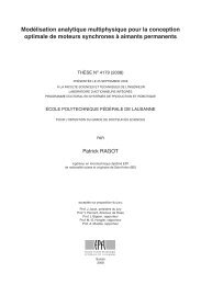
Figure 2.1: Elementary particle arrangements and particle assemblages (after Collins
and McGown, 1974): (a) individual clay platelet interaction , dispersed
structure, (b) individual clay platelet interaction, flocculated structure,
(c) clay platelet group interaction, turbostatic structure, (d) clay platelet
group interaction, bookhouse structure, (e) individual silt or sand interaction,
(f) clothed silt or sand particle interaction (g) particle assemblage
observed in variety of soils in three different types: (i) elementary particle arrangements
(ii) particle assemblages, and (iii) pore spaces.
Elementary particle arrangement consists of single forms of particle at the
level of individual clay, silt or sand particles or small groups of clay platelets or
clothed silt and sand particles. Occurrence of a single individual particle is rare
and usually platelets of clays tend to form a group of particles. Combination
of these arrangements forms different patterns of structure at the elementary
particle arrangement such as bookhouse and honeycomb as shown in Figure 2.1.
Elementary particles tend to group together rather than existence as individual
particles. These groups of elementary particles may regroup in larger order
and form what is termed here as particle assemblages. Depending on the type,
environmental conditions and origin of the structuring phenomenon (formation
of structures), different types of assemblages may exist. Connectors, for example,
are bridge-like assemblages that connect two (or more) other assemblages
which are usually of larger size.
Aggregates are other types of particle assemblages acting as individual units
in the structure. The cause for aggregation of particles and also size and shape
of aggregates may vary. According to Collins and McGown (1974), aggregation
might be found to be regular or irregular. In regular aggregation, unlike irregular
aggregation, aggregates have a definite physical boundary and therefore
particular hydro-mechanical properties can be attributed to aggregates themselves.
Particle matrices are also another type of particle assemblages which
form the background of the structure and depending on the extensiveness, in
some cases, act as a binder in overall soil structure. It is plausible to assume
that when special particle assemblages such as connectors, aggregates or interweaving
punches are destroyed and removed by any environmental cause, the
remaining structure of the soil contains mainly particle matrice assemblages.
Pore space is defined to be the space within and between the elementary
6
(g)

Background and problem addressing
particles and assemblages of particles. Volume of voids in soil is usually represented
by one of the following parameters: porosity, n, defined as the ratio of
void volume over the total volume of the soil, void ratio, e, defined as the ratio
of void volume over the volume of solid particles, or specific volume, v, which
is the total volume of soil which contains unit volume of solid particles. From
these definitions, it yields:
e = n
1 − n
(2.1a)
v = 1 + e (2.1b)
With respect to the classification of soil fabric, Collins and McGown (1974)
defined different pore classes as follow: (i) intra-elemental pores: pores within
the elementary particle arrangements, (ii) intra-assemblage pore: pores within
particle assemblages which may occur between sets of elementary particle arrangements
or between smaller particle assemblages within a larger assemblage,
(iii) inter-assemblage pore, pores between the particle assemblages, and (iv)
trans-assemblage pores, defined as being pores traversing the soil fabric without
any relationship to the individual micro fabric features.
This classification does not account for size; however, the nature of the
classifications adopted implies the absolute size to increase from intra-elemental
to trans-assemblage pore space. In certain types of soil fabric this classification
becomes simplified in single, double or multi-modal distributions for the pore
size.
2.1.2 Pore fluid
The pore space can be filled with a combination of fluids. The pore fluid in soils
is often comprised of water as the liquid and air as the gas phase. Dry and fully
saturated soils correspond to the two extreme cases when the pores are only
filled with air or water respectively. In soil mechanics, the intermediate states
of the soil in which the pores are filled with two (or more) fluids are termed as
unsaturated or partially saturated. In partially saturated soils, both the relative
proportion of liquid and gas occupying the pore space and the energy state of
the liquid phase has important influences on the mechanical response of the
material. The relative proportion of liquid and gas is represented by the well
known parameter of degree of saturation Sr defined as the ratio of pore liquid
volume over the total volume of the pores. The energy state, however, should
be evaluated in terms of water or liquid potential.
2.1.2.1 Pore water potential
Water potential is the potential energy of water relative to pure water in a
reference state. It quantifies the tendency of water to move from one area
to another due to osmosis, gravity, mechanical pressure, or capillary action.
An element of unsaturated soil, when in contact with a reference hypotethical
reservoir of free water, is capable of drawing water through the liquid and gas
7

Chapter 2
phase. In simple words, the term suction could be used to describe this property
(Tarantino and Jommi, 2005). More rigorously, the total suction in the soil refers
to the potential of soil water and it can be measured in terms of the partial
vapor pressure of the soil water (Richards, 1965; Fredlund and Rahardjo, 1993).
This is equivalent with the definition of total suction as the stress required
to extract a water molecule from liquid phase of soil matrix into the vapor
phase (Ridley, 1993, in Monroy (2005)). Many different potentials affect the
total water potential, and these effects are additive. In a simple system, two
components are the pressure potential and the solute potential.
(i) Pressure potential: The pressure potential corresponds to the intrinsic
pressure of the water which could be evaluated with respect to the atmospheric
reference pressure. In saturated soils, e.g. a soil element lying below the water
table, the water pressure is positive and the liquid is in compression. While,
in unsaturated soil, e.g. a soil element above the water table, the hydrostatic
water pressure is negative and therefore the liquid is in tension. This tension,
generated through the interaction of soil water and the soil matrix, is called
matric suction and it represents the pressure difference between the soil water
and the surrounding gas:
s = pa − pw
(2.2)
In the above relation, s denotes the matric suction, and pw and pa are water
and air pressure respectively. In most cases, the air pressure is the atmospheric
pressure and hence, the suction is equal to the negative water pressure.
The matric suction is a result of adsorption effects between soil and water
molecules and capillary action within the soil matrix. In the vicinity of soil
particles in unsaturated soil, the soil water is divided into capillary water and
adsorbed water. In soils with an aggregated structure, this could occur in the
vicinity of the aggregates or in the vicinity of primary particles within the
aggregates. The adsorbed water is tightly bonded to the soil particles and
could be considered as a part of solid skeleton (see e.g., Ma and Hueckel, 1993).
Contrary to capillary and adsorbed water, free or bulk water could move through
the pore space. At the condition of equilibrium, it is plausible to assume that
the water has the same pressure everywhere within the soil matrix.
Capillary action is a result of the liquid surface tension. Surface tension is
defined as the force along a line of unit length where the force is parallel to the
surface but perpendicular to the line.
The capillary effect can be demonstrated using the familiar example of capillary
tube. When the lower end of a vertical glass tube is placed in a liquid such
as water, a concave meniscus forms. Surface tension pulls the liquid column up
until there is a sufficient weight of liquid for gravitational forces to overcome the
intermolecular forces. The pressure difference at two sides of the water interface
with air are retained by the surface tension:
pa − pw = 2Ts
where rc is the radius of meniscus curvature and Ts is the surface tension.
8
rc
(2.3)

Background and problem addressing
(ii) Solute potential: Solute or osmotic potential of water is linked to the
dissolved solutes in soil water. Pure water is usually defined as having a solute
potential of zero, and in this case, solute potential of soil water containing dissolved
solutes can never be positive. The suction corresponding to this negative
water potential is called osmotic suction, sπ. The osmotic suction represents
the difference between the measured values of total water potential with respect
to two similar reference systems with free pure water and water identical
in composition with the soil water.
2.1.2.2 Suction in unsaturated soils
Following the description given above, the total suction, st, could be written as
st = s + sπ
(2.4)
in which s and sπ represent matric and osmotic suction in soil respectively. The
osmotic suction could be observed only if the soil water is in contact with pure
water through a perfect semi-permeable membrane which allows only the water
molecules to pass and not the solutes. Providing such a membrane is rather
complex and the osmotic suction is not usually measured in soils. However,
the concept of osmotic pressure, per se, has been used to design new testing
equipments for unsaturated clayey soils (Kassif and BenShalom, 1971; Delage
et al., 1998, among others).
The matric suction is widely accepted to be the governing component of
suction in description of the mechanical behavior of unsaturated soils, and it has
been used to formulate the mechanical constitutive models for these materials
(Alonso et al., 1990; Cui and Delage, 1996; Geiser, 1999). Accordingly, from now
later on in this study, the term suction refers to matric suction unless otherwise
stated.
2.1.3 Multi-scale heterogeneity
If the soil is idealized to be bundle of capillary tubes, the matric suction and the
meniscus formed at the particle contact point at the pore entrance is controlled
by Equation (2.3). However in reality, attention should be given to the soil
fabric and the heterogeneity of the soil matrix.
Most soils show different kinds of heterogeneity depending on the considered
scale. In classical soil mechanics problems, the level of heterogeneity is usually
limited to the differences among the characteristics of the soil layers. Inside
a specific soil layer at the scale of geotechnical testing samples, termed here
macro-scale, the soil is usually assumed to be homogeneous as soon as enough
grains or aggregates are considered. While at smaller scales corresponding to
that of the pores, here termed pore scale, heterogeneity can be defined by means
of smaller structural units, such as different pores, fissures or aggregates.
Postulation of a homogeneous soil at the macro-scale implies the consideration
of a representative elementary volume (REV) of a given material. A
REV is required to include a significant amount of small-scale heterogeneity to
9

Chapter 2
Figure 2.2: Effect of sample size on the porosity: (a) sample sizes (gray: solid, white:
void) (b) porosity vs. sample scale.
respect a meaningful statistical average (Vogel and Roth, 1998). As an example,
the dependence of the sample porosity on its scale is schematically shown
in Figure 2.2. It can be seen that the REV may be representative of a homogeneous
medium, while smaller samples are completely heterogeneous. For
volumes below the REV, as may be seen in Figure 2.2(a), the whole sample
can be located completely within the pores or within the particles, leading to
quite different values of porosity. However, when the sample sizes increase, the
difference between the two values of porosity decreases and they tend to a single
one obtained at the REV level. It is noteworthy that depending on the heterogeneity
of the medium at larger scales, the different measured values of a
parameter like porosity might again diverge at larger scales.
2.1.4 Structured soil
There is a strong relationship between the soil structure and soil heterogeneity.
In the classical soil mechanics, soil is considered to be a homogeneous continuum
in which heterogeneity at the pore and particle scale is usually smoothed out
(Laloui et al., 2003). It means that the effects of soil structure on its macroscopic
behavior is assumed to be insignificant. However in some soils, the response to
environmental loading is strongly influenced by the soil structure. These soils,
in general sense, are here referred to as structured soils. The behavior of these
materials are usually associated with special complexities in different aspects
that cannot be explained by classical soil mechanics theories without taking the
soil structure into account.
In the literature, soil structure effects on the material behavior have been
evaluated for two groups of soils: natural bonded soils where the inter-particle
bonding governs the material behavior, and aggregated soils including compacted
and expansive clays and, natural and agricultural aggregated soils in
which the soil fabric receives the main focus.
2.1.4.1 Natural bonded soils
Natural soils show various structures, characterized by structural units, such as
aggregates, porous block, fissures, earth worm holes and root channels. They
10

Background and problem addressing
differ from reconstituted soils, namely the soil with the same mineralogy from
which the structures are removed by remolding, in a number of important aspects.
The differences arise from their particular in-situ structure (Burland,
1990). The mechanical behavior of these materials is predominantly influenced
by inter-particle bonding. These materials are often referred to as natural structured
soils (Wood, 1995; Baudet and Stallebrass, 2004; Liu and Carter, 2000b;
Cuccovillo and Coop, 1999) or bonded soils (Gens and Nova, 1993; Nova et al.,
2003).
In these materials, different causes for development of bondings could be
considered; among them are solution and deposition of silica at particles contacts
in sands, cold welding at inter-particle contacts at high pressure, deposition of
carbonates, hydroxides and organic matter from solution, and the modification
of the adsorbed water layer and inter-particle attractive forces in clayey soils
(Leroueil and Vaughan, 1990). Although the cause of special structures in these
materials might be different and rather complex, according to Leroueil and
Vaughan (1990) the structural effects on the behavior could be described in the
same way.
In these materials, the bonds could be subjected to degradation and the
initial soil structure might change during different environmental loadings (see
e.g Callisto and Rampello, 2004). This phenomenon is referred to as structure
degradation or de-structuring. Reconstituted soil of the same mineralogy is
considered as the fully de-structured material and it is considered as reference
state to interpret the characteristics of structured soil (Burland, 1990).
2.1.4.2 Aggregated soils
Structured soils exhibit, in contrast to reconstituted soils, a wide and often bi- or
multi-modal pore size distribution. There are two extremes in conceptualizing
the fabric of these materials: aggregation of particles and macro void formation,
e.g., fissures, cracks or cavities.
Aggregation of particles results in an open structure for soil. The size of
aggregates ranges from tenths of microns to centimeters or even larger units
(clumps, clods). Soil aggregates in general may differ in properties such a
texture, resistance, porosity or relative density (Terzaghi et al., 1996). The
morphological characteristics of the pore space between the aggregates depends
on the size, distribution and shape of the aggregates and on their history of
formation and compaction.
The other extreme corresponds to the voids that form a continuous pore
space within a matrix. The openings (apertures) of such macropores are in the
order of some ten microns and larger. Fissures in swelling/shrinking soils, root
channels in forestry and arable soils and even bio-pores dug by the soil fauna
(e.g. earth worms) are main examples of macro void formation.
Aggregation of particles is a commonly observed phenomenon in natural
and agricultural soils (Horn, 2003) as well as in compacted clays at dry side
of optimum water (Barden and Sides, 1970; Sridharan et al., 1971; Collins and
McGown, 1974) and compacted expansive clays (Lloret et al., 2003). However,
11

Chapter 2
These soils tend to swell
(a)
Figure 2.3: Scanning electron microscopy of compacted clay at dry side of optimum
(Delage et al., 1996): (a) 300×, (b) 3000×
Incremental pore volume (ml/g)
0.2
0.16
0.12
0.08
0.04
0
Intra-aggregate
Dry density (Mg/m
1.8 1.5
3 )
Inter-aggregate
1 10 100 1000 10000 100000
Pore diameter (nm)
Figure 2.4: Distribution of incremental pore volume for two compacted bentonite
samples at different dry densities. Mercury Intrusion Porosimeter test
(Lloret et al., 2003)
size of aggregates in expansive and compacted clays are some orders of magnitude
smaller than aggregates in natural or agricultural soils. Figure 2.3 shows
the Scanning Electron Microscopy of clays compacted at dry side of optimum
in which aggregation of particles could be observed (Delage et al., 1996).
It has been observed that soils with an aggregated structure including compacted
clays (Al-Mukhtar, 1995; Delage et al., 1996; Griffiths and Joshi, 1990),
expansive clays (Gens et al., 1995) and natural aggregated soils (Cuisinier and
Laloui, 2004), are all characterized by a fabric with two dominant pore sizes corresponding
to micro- (intra-aggregate) and macropores (inter-aggregate). Figure
2.4 shows the bi-modal pore size distribution of an expansive clay obtained
by Mercury Intrusion Porosimetry. Hence, in the general sense, aggregated soils
are structured soils with double porosity.
12
(b)

Background and problem addressing
The hydro-mechanical properties of aggregates, as particle assemblages with
a definite physical boundary, could be to some extend treated separately from
the whole assembly of soil. These soils are termed double structure soil (Alonso
et al., 1999), as two levels of structure could be identified for these materials:
macro- and microstructure. The soil microstructure is defined as the elementary
particle associations within the soil aggregates, whereas the arrangement of
these soil aggregates and the relation among the structural units at the aggregate
level is referred to as the macrostructure (Al-Mukhtar et al., 1996). The
micropores or intra-aggregate pores are considered to be the smaller capillaries
and pores within the aggregates and their vicinity; whereas, macropores or
inter-aggregate pores are the much larger intercluster voids between the aggregates.
However, the boundary between micropores and macropores is arbitrarily
chosen in the literature with vague criteria (Kodikara et al., 1999).
2.1.5 Concept of double porosity
Such a division of pores into macro and micro levels leads to the concept of
double porosity for soils. This concept has been extensively used in different
fields and it can address the both features depicted in Figure 2.5.
The concept of double porosity was first introduced by Barrenblatt et al.
(1960) as a flow model for non-deformable fissured porous media. This model
was simplified by Barrenblatt (1963) and Warren and Root (1963). Then Aifantis
(1977) extended this concept by sketching the basis of a multi-porosity model
to include mass exchange of solutes through diffusion between the mobile and
stagnant water phases. The general theory of Aifantis unified the earlier proposed
models of Barenblatt for fluid flow through non-deformable porous media
with double porosity and Biot’s theory for consolidation of deformable porous
media with single porosity (Biot, 1941). This theory was widely applied to
model the consolidation phenomena in fissured clays and deformable fractured
media (Wilson and Aifantis, 1982; Musso et al., 1990; Khalili and Valliappan,
1991; Ghafouri and Lewis, 1996; Khalili et al., 1999; Callari and Federico, 2000).
A new coupling link between the elastic volumetric deformations of the two pore
systems was added by Khalili and Valliappan (1996).
Figure 2.5: Concept of double porosity: (a) Aggregated soil; (b) Fissured porous
medium
13

Chapter 2
The concept of double porosity has been also used in analysis of multiphase
flow related to petroleum reservoirs in fractured media (Lewis and Ghafouri,
1997). It has been also widely used in description of the behavior of swelling
materials (Alonso et al., 1991; Gens and Alonso, 1992; Alonso, 1998; Sanchez
et al., 2005).
Parallel to the problems of deformation, double porosity models are also
widely used in solving problems of water and solute transport in soil. In such
media, water flows preferentially through the macropores (Gwo et al., 1995;
Simunek et al., 2003) and this results in more complex water flow in the media.
In the existing models for flow in double porosity media, the porous medium
is assumed to be a system of two overlapping interacting regions associated
with macro- and micropores (Simunek et al., 2001; Huang et al., 2003). Although
most of the fluid mass is stored in the micropores, the permeability of
the macropores is much higher than that of the micropores (Tuncay and Corapcioglu,
1995). This concept leads to models in which two distinct pore pressures
are present in two system of pores (Wang and Berryman, 1996).
Two different approaches exist for water flow in a double porosity medium:
dual permeability and dual-porosity approach (e.g. Gerke and Van Genuchten,
1993). The first one allows for the water to flow in both macropores and the
matrix. Darcy’s law is postulated for both systems of pores with different values
of permeability providing additional terms for water transfer between macroand
micropores. This approach has been used for the study of consolidation in
double porosity media (Wilson and Aifantis, 1982; Musso et al., 1990; Lewallen
and Wang, 1998; Khalili et al., 1999; Callari and Federico, 2000) and water flow
in deformable double porosity soils (Khalili and Valliappan, 1996; Lewis and
Ghafouri, 1997; Lewandowska et al., 2004). The second approach assumes that
water flow happens only through the macropores. Micropores are assumed to
be only involved in the local water exchange between two system of pores and to
act as feeding sources for macropores that can exchange, retain and store water
but do not permit convective flow (Huyakorn et al., 1983; Simunek et al., 2003).
As a result, water in aggregated soil is either mobile water, namely free bulk
water in macropores, or immobile water in micropores within the aggregates
(Gwo et al., 1995; Pini and Putti, 1997; Simunek et al., 2001; Huang et al.,
2003; Simunek et al., 2003). The immobile water in intra-aggregate pores is
considered by some authors as the water adsorbed by solid particles that should
be treated as a part of solid phase (Loret et al., 2002; Ma and Hueckel, 1993;
Murad and Cushman, 2000). Each approach requires its own set of appropriate
hydraulic constitutive equations that should be introduced to derive the field
equations.
Recently, Sanchez et al. (2005) developed the formulation of double porosity
media applied to an aggregated expansive soil consists of clay pellets. They used
the conceptual model of Ghafouri and Lewis (1996) in which the medium with
double porosity is divided into two overlapping but distinct continuum corresponding
to two different structures of pores. The first one is related to the solid
particles and the voids inside the pellets, and the second medium is associated
with the pellets and the pores between them. Although, this concept offers
14

Background and problem addressing
different possibilities to better describe problems of double porosity media, it
suffers from the fact that degradation of structures and structure modifications
are not integrated in it.
2.2 Partial saturation effects
2.2.1 Water retention characteristics
The relation between the the liquid potential and the relative proportion of
liquid and gas occupying the pore space in unsaturated soils is evaluated by the
soil water retention characteristics. For a soil with given void ratio and fabric,
the degree of saturation, Sr, in the isothermal condition depends on suction
s. In general, the relation between degree of saturation (Sr), suction (s), and
void ratio (e) identifies the water retention characteristics of a soil and the plots
representing this relations are called water retention curves.
Water retention curve of unsaturated soils has been studied both in soil
physics (Van Genuchten, 1980; Green et al., 1996) and soil mechanics (Sivakumar,
1993; Geiser, 1999; Cunningham et al., 2003; Tarantino and Tombolato,
2005, among others). Figure 2.6 presents the experimentally determined relation
between degree of saturation, suction, and void ratio for London Clay
during drying and wetting under constant external stress (Cunningham et al.,
2003).
In general, and as it can be seen in this figure, the degree of saturation
decreases with suction. However, experimental observations have shown that
the degree of saturation for a given suction is not identical in drying and wetting
path. This phenomenon corresponds to the hydraulic hysteresis (Croney, 1952).
The hydraulic hysteresis should be ascribed to the fabric of soil and the different
effects of pore entrapments in drying and wetting paths.
When a sample of saturated soil is subjected to suction increase at constant
Degree of saturation S r
1 . 2
0
0 . 8
0 . 6
0 . 4
0 . 2
1
0
10 100 1000 10000 100000
. 44
1 . (a) (b)
42
10 100 1000 10000 100000
Suction, s: kPa
Virgin drying
Wetting
Specific volume, v(1 e)
1 . 54
1 . 52
1 . 5
1 . 48
1 . 46
Suction, s: kPa
Figure 2.6: Water retention curve for a clay-silt mixed soil (Cunningham et al.,
2003): (a) degree of saturation-suction, (b) specific volume-suction
15

Chapter 2
Specific volume, v
2 . 4
2 . 3
2 . 2
2 . 1
2 . 0
a
c
e
1
10 100 1000
. 9
Mean net stress, p u a : kPa
(a)
b
d
Degree of saturation, S r
c
a
e
0
10 100 1000
. 5
Mean net stress, p u a : kPa
Figure 2.7: Behavior of bentonite-kaolin during isotropic loading at constant suction
(Sharma, 1998, in Wheeler et al. (2003)): (a) specific volume, (b) degree
of saturation
external loading, the pores remain saturated until a given suction (Blight, 1967;
Geiser, 1999, among others). This suction is called air entry value suction and
it is usually denoted by se. When this limit is surpassed, the soil enters a
quasi-saturated state in which occluded air bubbles exist in the soil with the
water menisci being formed at the boundary of bubble with the bulk water
(Tarantino and Jommi, 2005). After this state, the degree of saturation of the
sample continues to decrease in a partially saturated state until a residual value
Sres termed as residual degree of saturation. At the residual state, only small
water menisci with high values of negative water potential exist within the soil.
The explicit dependence of degree of saturation on void ratio has been usually
ignored. When dealing with the assumption of incompressible material, the
consequences are limited. However, experimental results on real deformable soil
show that an increase in void ratio (even at constant suction) could increase the
degree of saturation in soil (Sivakumar, 1993; Sharma, 1998; Monroy, 2005).
An example of such behavior is presented in Figure 2.7 for unsaturated
bentonite-¨kaolin during isotropic compression under constant suction. The
mean net pressure in these figures is the total pressure from which the air
pressure has been subtracting and it represents the mechanical loading applied
to the soil.
Equivalent increase of degree of saturation was observed by Cuisinier and
Laloui (2004) during the oedometric compression of aggregated silt at constant
suction. In natural aggregated soils, macropores are usually drained even at low
values of suction. When these empty pores are closed as a result of mechanical
loading, the total volume of voids are modified while the mass and volume of water
in the aggregates remains almost constant. Hence even at constant suction,
the degree of saturation could be subjected to significant increase depending on
the state of compression.
A direct consequence of suction increase, in general, is shrinkage of the soil.
Different interpretations have been given for the volume change of soils with
16
1 . 0
0 . 9
0 . 8
0 . 7
0 . 6
(b)
b
d

s
Suction,
A
B
C
Mean net pressure
(a)
e
Void ratio,
A
C
κ s
κ s
λs
sy
Suction (log scale)
(b)
Background and problem addressing
B
e
Void ratio,
A
λs
κ s
s s e y
Suction (log scale)
Figure 2.8: Typical interpretations for suction-induced volume change: (a) drying
path, (b) interpretation of Alonso et al. (1990), (c) interpretation of
Geiser (1999)
suction increase (Fig. 2.8). Alonso et al. (1990) suggested for a soil in a drying
path, an elastic deformation until reaching a yield suction beyond which plastic
volume change occurs in the same way as in an isotropic mechanical loading path
(Fig. 2.8(b)). If the soil is then subjected to wetting, it again follows an elastic
path like mechanical unloading. In line with definition of preconsolidation stress,
the yield suction (sy) in this interpretation is considered to be the maximum
previously experienced suction.
Another interpretation, given by Geiser (1999) who evaluated the experimental
results of Zehrouni (1991) and Taibi (1994), appears to be more realistic. In
this interpretation, depicted in Figure 2.8(c), the suction-induced deformations
are mainly irreversible in the domain of saturated pores and reversible in the
domain of unsaturated pores. The yield limit suction, sy, is allowed to be equal
to or slightly different from the air entry value suction, se. In this latter case,
the yield suction has been linked to the shrinkage limit of the soil.
The slopes of reversible and irreversible parts, in both interpretations, are
considered to be material properties.
2.2.2 Capillary effects
The capillary effects could be evaluated through the concept of water meniscus.
According to Gens and Alonso (1992), the water menisci could be present at
the particle contact between individual sand and silt grains or between the soil
aggregates. The effects of the water meniscus on the mechanical behavior of the
soil at the macro-scale have been discussed by several authors (Tarantino and
Tombolato, 2005; Jennings and Burland, 1962, among others). It is commonly
accepted that the water meniscus could act as bonding between soil particles,
retains the soil particles together, and therefore, enhances the overall stability
of the soil skeleton.
One of the major consequences of the presence of inter-particle menisci in
partially saturated soils is dependency of yield limit, during loading at constant
suction, on the suction level (Wheeler and Sivakumar, 1995; Alonso et al., 1987,
C
(c)
B
17

Chapter 2
among others). In general, the higher the tensile pressure of water meniscus,
the higher the yield limit in unsaturated soil. This implies the yield limit to be
a function of not only stress state and stress history, but also of suction.
Another important effect of water menisci is collapse upon wetting of unsaturated
soils (see e.g. Wheeler and Sivakumar, 1995). This phenomenon is
linked to the removal of water menisci and capillary effects at saturated state.
Logically, it is plausible for the soil rigidity to be affected by the presence of
water menisci in the unsaturated soils. The influence of suction on soil rigidity
will be reflected in the elastic modulus and the mechanical compressibility.
It has been repeatedly suggested for the elastic properties to be independent
of or insignificantly dependent on suction (Geiser, 1999; Rifa’i, 2002). Accordingly,
a constant slope of unloading-reloading is usually considered in the
compression space of v − ln pnet (pnet is the mean net pressure). However, some
authors argued that this slope increases with suction (Al-Mukhtar et al., 1993).
The mechanical compressibility in unsaturated soils has been often evaluated
by studying the influence of suction on the slope of normal consolidation line in
v − ln pnet space. Most authors agree in the fact that this slope decreases due
to the suction increase (Matyas and Radhakrishna, 1968; Alonso et al., 1987;
Charlier et al., 1997; Sivakumar, 1993; Geiser, 1999). However, some authors
argued that the evolution of this slope with suction depends on the suction
level and stress state of the soil (Wheeler and Sivakumar, 1995). Hence, the
understanding of the evolution of soil compressibility with suction still demands
more rigorous investigations.
2.3 Fabric effects in unsaturated soils
2.3.1 Influence on water retention characteristics
The influence of fabric on the water retention characteristics has been evaluated
for natural aggregated soils (Coppola, 2000; Burger and Shackelford, 2001) as
well as for compacted clays at dry side of optimum and compacted expansive
soils (Romero et al., 1999, among others). As previously mentioned, these
materials exhibit double porosity fabric; therefore, some understanding of fabric
effects in these materials is helpful in the current study.
Figure 2.9 shows the evolution of volumetric water content with suction
for a specimen containing pellets of about 1 mm diameter from processed diatomaceous
earth reported by Burger and Shackelford (2001). The results are
presented in terms of volumetric water content (the fraction of the total volume
of soil that is occupied by the water contained in the soil). The measured soilwater
characteristic curve data are bimodal, reflecting both the microporosity
region within the individual pellets, or intra-pellet porosity, and the macroporosity
region between the pellets, or inter-pellet porosity. These authors introduced
the inflection point in the bimodal water retention curve (Fig. 2.9(b)) as the
point where the macroporosity appears to have completely desaturated and the
microporosity begins to desaturate. They suggested that the water retention
data for soil suctions greater than, and less than the suction corresponding to
18

(a) (b)
Background and problem addressing
Figure 2.9: Bimodal soil-water characteristic curve (Burger and Shackelford, 2001):
(a) measurements and fits for specimens containing pellet processed diatomaceous
earth, (b) schematic of a conceptual representation
Figure 2.10: Main wetting and drying retention curves for the different packings of
compacted Boom clay (Romero et al., 1999)
this point could be evaluated separately according to the physical properties of
macro- and micropores. In the joint study of the present research work, Carminati
(2006) studied the water retention properties of aggregates and micropores
within them. Results of that work showed that the water retention behavior of
aggregates are influenced by different factors such as the geometry of pores and
aggregate contacts.
Figure 2.10 illustrates the relation between degree of saturation and suction
for different packings of a compacted Boom clay, a material with initial double
porosity fabric (Romero et al., 1999).
19

Chapter 2
The water retention curve of the aggregated clay in Figure 2.10 shows two
regions with different responses to change in void ratio. At lower values of
suction, dependence of retained water on soil void ratio (dry density) is observed;
however, at higher suctions, the retained water is independent of soil void ratio.
Romero et al. (1999) associated these two regions with intra- and inter-aggregate
governing suction zones. They discussed that in the inter-aggregate governing
suction zone, the water content is high enough to partly fill the inter-aggregate
voids. This zone is sensitive to mechanical actions, since the mechanical loading
reduces the macroporosity and affects the bulk water contained in the interaggregate
pores. While, the intra-aggregate porosity is not significantly affected
by this effect.
Equivalent observations of two regions were made by Lloret et al. (2003) for
the water retention curve of compacted bentonite. They reported that the region
of high suctions in the water retention curve corresponds to the intra-aggregate
pores, where total porosity plays no relevant role and the water uptake is mainly
governed by electro-chemical forces. Bernier et al. (1997) and Cuisinier and
Masrouri (2004) expressed similar explanations for their experimental evidence
in which retained water at high suctions appeared to be independent of dry
density for compacted clay.
Theoretically, the macropores require lower suction, in comparison with micropores,
to be drained (Eq. 2.3). Accordingly, there is a possible suction state
at which the macropores are drained while the micropores are still saturated.
With respect to this point, Gens and Alonso (1992) postulated the assumption
that clay aggregates in compacted expansive soils remain saturated, whatever
the state of the soil would be, and therefore their behavior could be described
using saturated soil concepts.
2.3.2 Collapsible behavior
A possible scenario during the wetting of aggregated soils is the removal of
inter-particle bondings and disintegration of soil aggregates.
It is noteworthy that in the case of compacted material, the bonding could
be either strong inter-particle water menisci or electro-chemical forces. Removal
of these bonds yields the collapse of the aggregated structure and consequently
results in dramatic deformations of the whole soil.
Observations made by Alonso et al. (1995) during the soaking of expansive
clay pellet samples under constant vertical stress showed that the applied confining
stress plays an important role on the response of aggregated structure
upon wetting. In these tests, carried out in conventional oedometer cells, specimens
were soaked under vertical loads in the range of 10 kPa to 2.4 MPa and
the real time deformations were recorded, as presented in Figure 2.11.
For the samples wetted at low confining stress, clay pellets were found to
expand because of their expansive nature. In these samples, an increase in void
ratio could be observed up to a certain point where aggregates and subsequently
the soil at the macro-scale collapse. However, the final deformation was reported
to be a swelling strain.
20

Background and problem addressing
Figure 2.11: Soaking of compacted Boom clay samples under different vertical loads
for dry unit weight of 13 kN/m 3 (Alonso et al., 1995)
When confining stress increases, swelling tendency of aggregates is masked
by their distortion and collapse of aggregates; therefore, void ratio of soil starts
to decrease from the beginning of wetting. It was observed that reduction in
void ratio happens in two main steps. This behavior was attributed to the
wetted aggregates occupying the empty macropores at the first step and then
to the overall collapse of the soil structure at the second step. It is also observed
that the time or average suction for the outset of collapse decreases as confining
stress increases.
Hoffmann et al. (2006) showed that the required time for collapse of a compacted
clay specimen during wetting is controlled by the rate of application of
moisture at the specimen boundaries. They reported an immediate collapse of
specimens wetted by liquid water, while the collapse of specimens wetted by
vapor happened later.
Interpreting their experimental observations, Hoffmann et al. (2006) stated
that in the case of slow application of suction variations, water potential at
micro- and macropores have the opportunity to remain equal through the wetting
process and this prevents a sudden collapse before the condition close to
saturation.
These observations could be compared with those made by Or (1996) who
stated that major deformation of agricultural aggregated soil during wetting, in
presence or absence of external load, is due to wetting-induced disintegration of
aggregates at the top layer of the soil.
21

Chapter 2
2.4 Inter-particle bonding effects
Experimental evidence of the bonded soil structure effects on the mechanical
response have been reported for a wide variety of natural soils, including soft
rocks (Tavenas and Leroueil, 1990; Smith et al., 1992), stiff clays and clay shales
(Calabresi and Scarpelli, 1985; Anagnostopoulos et al., 1991; Burland et al.,
1996), granular soils (Mitchell and Solymar, 1984; Coop and Atkinson, 1993)
and residual soils (Vaughan and Kwan, 1984; Vaughan et al., 1988; Wesley,
1990). In almost all of these works, the influence of soil structure has been
evaluated with respect to inter-particle bonding effects and explicit investigation
of soil fabric has been rarely done (Cuccovillo and Coop, 1999). Furthermore,
study of this works has been mainly limited to the saturated states. To identify
the extra features in the mechanical behavior of natural soils arising from soil
structure, it is widely accepted to compare it with reconstituted soil of the same
mineralogy as a reference state. Burland (1990) should be cited as the first one
who suggested the term intrinsic for properties of the reconstituted soils, a
terminology which has been widely used by others in further works in this field.
2.4.1 Pre-yield behavior
The pre-yield behavior of soils is commonly characterized by the elastic (recoverable)
deformations. Influence of soil structure on the elastic properties has
been evaluated by Callisto and Calabresi (1998) who compared the behavior
of structured Pisa clay with the corresponding reconstituted samples. They
reported a fair agreement between the elastic stiffness of the reconstituted and
structured clay for small stress increments. This implies for elastic properties to
be independent of the soil structure. The assumption of independence of elastic
behavior from the soil structure has been a common postulation in development
of constitutive models for structured soils (Gens and Nova, 1993; Rouainia and
Wood, 2000).
However, Leroueil and Vaughan (1990) argued that although behavior before
the primary yield is stiff, it is not necessarily elastic. These authors, based on
the experimental observation of Bressani and Vaughan (1989), reported that
structure may be destroyed and yield stress reduced while a sample is following
a stress path within the primary yield limit.
2.4.2 Yield limit
In an intact state, the inter-particle bonding could enhance the overall stability
of the soil skeleton, hence, it is logical for the strength and the yield limit of the
soil to increase due to presence of these bondings.
The yield limit in isotropic compression condition is represented by the normal
consolidation line. For a reconstituted saturated soil, all possible states lie
to the left side of this curve in a v −p ′ space where p ′ is the mean effective pressure.
However, experimental observations proved that the virgin compression
curve for most of sedimentary natural soils lie well above the normal consolida-
22

Background and problem addressing
(a) (b)
Figure 2.12: One-dimensional compression of natural structured and reconstituted
clays: (a) Bothkennar Clay, natural clay taken with two different different
samplers (Smith et al., 1992), (b) Pisa clay (Callisto and Calabresi,
1998)
tion line of reconstituted soil (Burland, 1990).
Effects of bonded structure with respect to this fact have been examined
by Leroueil and Vaughan (1990) for different natural soils. They reported that
many of the naturally occurring sedimentary and residual soils have components
of strength which cannot be accounted for by porosity and stress history alone.
Leroueil and Vaughan (1990) showed that the void ratio for both residual and
sedimentary structured soils is greater than can be sustained by the same soil
from which structure has been removed by remolding. Similar observations were
made by Smith et al. (1992) who studied the yielding behavior of Bothkenar
natural clay. They compared the oedometric compression curve of undisturbed
Bothkenar clay with the compression curve of reconstituted soil termed as intrinsic
compression curve (ICC), as presented in Figure 2.12(a). These authors
reported a higher oedometric yield stress for the structured clay. For a given
stress, this allows the structured clay to sustain higher void ratio in comparison
with reconstituted soil. Equivalent observations were made by Callisto and Calabresi
(1998) for the oedometric compression of both natural and reconstituted
Pisa clays, as presented in Figure 2.12(b).
The observed behavior of structured natural clays can be often reasonably
approximated by straight pre-yield and post-yield segments (Graham et al.,
1988). Leroueil and Vaughan (1990) stated that while bonded structure in
these materials might arise from different causes, its consequences on the material
behavior is similar and corresponds to a stiff behavior followed by yield.
Accordingly, they described this yield in a similar way to that occurring due to
overconsolidation, although it is a different phenomenon.
23

Chapter 2
Void ratio
A
C
decreasing rate of
deformation
B
creep
Vertical effective stress (log scale)
Figure 2.13: Effect of creep on one-dimensional compression of clay (after Wood,
1990)
The apparent overconsolidation behavior of bonded soils could be compared
to the effects of creep and aging in soils (Bjerrum, 1972). The term creep is
usually used to describe deformation continuing with time at constant effective
stress. The description given by Wood (1990) is adapted here for the relation
between creep and the apparent overconsolidation behavior. If an oedometer
test (AB in Fig. 2.13) is stopped in the middle of the test, creep occurs (BC). As
the rate of creep deformation gradually falls with time, the state of the soil moves
to lower compression curve appropriate to the falling rate of deformation.When
the loading is restarted, state of the soil returns back to the compression curve
following which it had been loading from the beginning of the test (CDE).
Therefore, sample appears to have become apparently overconsolidated and an
apparent preconsolidation pressure would be assigned to D (in Fig. 2.13) even
though the soil had never previously experienced effective stresses higher than
those at B (in Fig. 2.13) and C. This description could explain the behavior of
marine deposits and aged soil in which creep have been occurring in large scales
of time.
The relation between creep and the soil structure has been studied by some
authors (Leroueil, 2006; Sorensen et al., 2007). However, further evaluation of
this relation is beyond the scopes of this study and will not be treated here.
2.4.3 Yielding behavior
The inter-particle bonding has been found to have a major effect not only on
the yield limit but also on the post-yield and the material response during the
occurrence of yielding.
Burland (1990) showed that natural sedimentary clays are more sensitive
and they exhibit a more brittle behavior than reconstituted material and the
post-yield compression index is usually much greater in natural soils. It has been
reported that the compressibility index for structured soft clay correlates with
initial void ratio and the sensitivity of the clay rather than with plasticity in
24
D
E

Background and problem addressing
conventional manner (Leroueil et al., 1983). Brittle behavior was also observed
in the compression behavior of natural Bothkennar clay by Smith et al. (1992).
They identified a sharp yielding corresponding to the transition from recoverable
to irrecoverable domain of material behavior in various stress-path triaxial tests.
In the case of natural Pisa clay, however, triaxial and oedometer results of
Callisto and Calabresi (1998) showed that the yielding in this material is a gradual
phenomenon. While, the post-yield compression curve of natural clay was
still characterized by greater compressibility value in comparison with reconstituted
soil. They ascribed the increase in the compressibility to a progressive
change in the microstructure of the clay. They showed that when the stress
path involves greater changes in the deviatoric stress than mean pressure, the
behavior of reconstituted and natural material is qualitatively similar. While,
the behavior of the two soils are different for stress paths where the reverse
change of stress applies.
It has been commonly reported that the compression curve of structured clay
tends to converge to that of reconstituted clay, as the applied stress increases
(Burland, 1990; Callisto and Calabresi, 1998). As expressed by Graham et al.
(1988), after Bjerrum (1967), in the region between the pre-yielding and postyielding
the microstructure of natural clays experiences major disturbance or destructuring.
Consequently, the influence of soil structure becomes less important
and the response of the materials becomes closer to that of the reconstituted
soil without inter-particle bonding.
Leroueil and Vaughan (1990) argued that the complete removal of structure
does not necessarily imply coincidence of the compression curves of structured
and reconstituted soil and further strains might be required to achieve similar
fabric and particle packing. Rouainia and Wood (2000) also discussed that the
occurrence of localization in these materials will prevent any further homogeneous
de-structuring and only within the zone of concentrated shearing, loss of
structure will be completed. Therefore, it will not be possible to deduce the
asymptotic behavior of reconstituted materials.
Microstructural study of natural clays has shown that some elements of
structure remain in the clay even at very large strains or after reconstituting
(Cotecchia and Chandler, 1998). This can be better described using the concept
of metastable fabric for sedimentary soils (Mitchell and Soga, 2005). In
these materials, the initial fabric after deposition is quite open with large pores.
During consolidation this fabric can carry effective stress at a void ratio higher
than would be possible if the particles and particle groups were arranged in
an efficient parallel arrangement (Mitchell and Soga, 2005). When the soil is
remolded, the fabric is progressively disrupted and the strength is decreased.
Compression of the initial metastable state corresponds to the virgin compression
of the soil, as depicted in Figure 2.14(a). States to the right side of this
curve would be possible only in the presence of bondings which enables the soil
to resist additional compressive stress (ab) or to exhibit additional void ratio
(bc). While, the difference between the virgin compression of metastable state
and the compression of fully de-structured soil, namely cd, is ascribed to the
soil fabric.
25

Chapter 2
(a)
lnv n
ICL
Line representing in-situ
states of natural soil
Bonding
Fabric
Stable structure
Metastable
structure
Figure 2.14: Effects of bonding and metastable fabric on the compression of clays
(a) possible states in void ratio-effective stress plane (Mitchell and Soga,
2005), (b) the difference in behavior of clays with stable and metastable
structure in compression (Baudet and Stallebrass, 2004)
Figure 2.15: Compression behavior of structured and reconstituted soil (Leroueil and
Vaughan, 1990)
Using this concept, Baudet and Stallebrass (2004) divided the soil structure
into stable structures that do not degrade; and metastable structures which undergo
de-structuring (Fig. 2.14(b)). They reported that the convergence toward
intrinsic states is characteristic of natural clays with metastable structure. For
clays with stable elements of structure, it is hypothesized that no strain path
could ever achieve a level of de-structuration that would bring it to the intrinsic
state. In such case, they considered that the soil could reach a stable state that
is not the intrinsic state due to existence of stable elements in the soil fabric.
In general, as proposed by Leroueil and Vaughan (1990), compression curve
of structured soil and reconstituted soil from loosest possible state could be
simplified as depicted in Figure 2.15. They introduced a structure permitted
space for structured soils, in which soil can exist only due to structure.
26
(b)
ln p′

Background and problem addressing
2.4.4 Combined effects of bonding and partial saturation
Although many natural structured soils are unsaturated, only few studies have
considered the combined effect of unsaturation and bonded soil structure on
soil behavior. These effects were discussed by Alonso and Gens (1994) for the
purpose of constitutive modeling. To our knowledge, the only representative
experimental research in this field is the work done by Leroueil and Barbosa
(2000). These authors examined the combined effects of bonding and partial
saturation on yielding of artificially cemented soils and non-cemented soil by
means of triaxial and oedometer tests. Despite the difference between the nature
of tested material and the structured soil concerned in this study, the results
of that work provide a background about the suction effects in bonded material.
They examined the oedometric yield stress of cemented and non-cemented soil
at different suctions. The yield stresses deduced from their tests are plotted in
Figure 2.16 in the space of suction versus the vertical net stress. The increase
due to suction of yield stress in reconstituted soil (∆σy,suc) is determined by
curve LCa, named Loading-Collapse curve after Alonso et al. (1990). At saturated
condition, cementation induces an additional increase in the yield stress
(∆σy,st). If this value is added to the curve LCa, the dashed line is obtained.
However, yield stress given by the obtained curve appeared to be less than the
real yield stress for unsaturated cemented soils. The difference (∆σy,suc) has
been attributed to the hardening effect of suction on bondings. Therefore, they
showed that the yield stress resulting from the combined effect of partial saturation
and bonding is larger than the sum of the contribution of the two factors.
As observed in these results and proposed by Alonso and Gens (1994), suction
in bonded soils has two effects corresponding to capillary effects on soil matrix
and strengthening of inter-particle bonds which should be taken into account
when dealing with these materials at unsaturated states.
Figure 2.16: Loading-Collapse curves for cemented and non-cemented Viçosa residual
soil Leroueil and Barbosa (2000)
27

Chapter 2
2.5 Study of soil structure
2.5.1 Experimental methods for soil fabric study
Over the few recent years, experimental study of soil structure has received an
increasing interest with the purpose of relating the soil structure at the pore
scale to the macroscopic behavior.
There are several ways to study the structure of geomaterials, among them
being scanning electron microscopy, nitrogen adsorption, mercury intrusion
porosimetry (MIP) and new methods based on computed tomography.
In general, these techniques are aimed at evaluating and characterizing the
soil fabric and they provide information about the geometry of pores and particles
in soil. These techniques can be classified according to several criteria.
These criteria include the direct or indirect and the destructive or nondestructive
nature of the method and also the type of obtained information
and the measured porosity. They might provide information on total porosity
or on connected porosity with only the mere knowledge of the global porosity
or with additional three-dimensional information about the connected porosity
pathways (Pleinert and Degueldre, 1995).
Technically, experimental methods involved in the study of soil fabric can be
divided into two main categories: direct and indirect methods. In the first group,
as the name indicates, the evaluation of soil fabric is based on direct observation
of the geometry of the pores using images. This includes for example optic or
electron microscopy. For the indirect methods, usually a second material is
injected into the pores and the geometrical information of pores is related to a
physical measurable variable of the material in contact with soil. The methods
usually give quantitative information about the soil fabric. The most popular
technique of the latter type is the mercury intrusion porosimetry (Sridharan
et al., 1971). Using mercury intrusion porosimetry combined with scanning
electron microscopy as a supplement has been the most popular approach to
study the soil fabric (Monroy, 2005; Delage and Lefebvre, 1984; Romero, 1999).
Recently, new advanced experimental methods based on radiography and
computed tomography (CT) have been used to evaluate the structure and the
physical and mechanical properties of geomaterials in different fields. Radiography
allows evaluating the soil texture and disturbance; while, CT allows
reconstruction of a three-dimensional volume of the sample by assembling twodimensional
radiographic images taken at different angles.
The most commonly used method of this kind is X-ray CT and radiography
(see e.g. Otani, 2006). X-ray radiography has been used to evaluate the physical
properties of geomaterials in different fields. Peyton et al. (1992) and Zeng et al.
(1996) used the X-ray radiography to evaluate the macro pore size and bulk
density in undisturbed samples of soil. The method has been also used to assess
the distribution of pores in samples of sand and cemented clays (Anderson and
Hopmans, 1994). X-ray tomography has been used to evaluate the evolution of
density and pore structure in soils and the crack propagation in rocks (Desrues
et al., 1996; Alshibli et al., 2000; Wong, 2000; Otani et al., 2000). A discussion
28

Background and problem addressing
of using X-ray CT for geotechnical engineering is given in Otani (2006).
Neutron radiography and tomography is another method of this type which
has been recently used for geomaterials. The main advantage of neutron radiography
to X-ray is its high sensitivity to hydrogen-containing materials and its
ability to track the water in soil. Neutron radiography has been used to image
both fluid infiltration into dry sand and steady state flow fields with the purpose
of measuring wetting front velocity and hydraulic conductivity of the medium
(Deinert et al., 2002). Combination of neutron radiography and tomography
has been also used for some experiments in order to evaluate the influence of
initial moisture content and type of infiltrating fluid on the formation of preferential
flow paths (Tullis et al., 1992). Neutron tomography has been also used
to study the variation of fluid saturation in sandstone samples and relate it to
the pore geometry (Solymar et al., 2003). In the joint study of the present
work, Carminati (2006) used neutron radiography and tomography in order to
study the water retention behavior and water flow in series of aggregates. As
it will be presented later, this technique is as well used in the present work for
non-destructive study of soil structure. Detailed description of the employed
method and the testing procedure are given in Chapter 5.
Each method of soil structure study has its own requirements and testing
condition. For example, MIP or SEM are destructive methods and their application
is limited to small samples. CT methods could provide morphological
information of larger samples with the price of higher costs and usually lower
resolution. As proposed by Mitchell and Soga (2005), the use of several methods
of fabric analysis may be appropriate in some cases in order to obtain information
of more than one type or level of detail.
2.5.2 Fabric evolution
In the case of structured double porosity soils, a few studies have been undertaken
to characterize the fabric evolution during the mechanical loading or
suction variations. One point of interest has been the fabric modifications provoked
by mechanical loading under saturated condition. Delage and Lefebvre
(1984) studied non-compacted Champlain clay fabric with mercury intrusion
porosimetry (MIP) and scanning electron microscopy. This material shows an
initial double porosity fabric. The results showed that during consolidation
only the largest pores collapse at a given stress increment. Small pores are
compressed only when all of the macropores have been completely closed by
loading. These results were confirmed by similar evidences in other experimental
studies (Lapierre et al., 1990; Griffiths and Joshi, 1990).
Soil fabric is sensitive to suction increase, as evidenced by Simms and Yanful
(2001, 2002) who investigated the fabric of a compacted glacial till under different
suctions, from saturation up to a matric suction of 2500 kPa. They showed
that increase of suction brought about a progressive rise in the microporosity
associated with macroporosity reduction. They modified the measured pore
size distribution for pore trapping effects and proposed a model for shrinkage
of pores and evolution of pore size distribution due to drying.
29

Chapter 2
(a)
(b)
Figure 2.17: Fabric modification due to mechanical loading and suction variations:
(a) suction increase at constant net vertical stress 10 kPa, (b) mechanical
loading under saturated condition (Cuisinier and Laloui, 2004)
Cuisinier and Laloui (2004) studied the combined effects of suction and
mechanical loading on the fabric of unsaturated aggregated silt. Figure 2.17
shows the pore size distribution of the tested samples at different levels of applied
net stress and suction. The results confirmed that mechanical loading affects
mainly the macropores. They also showed that suction increase is associated
with decrease in the volume of macropores and a slight increase in the volume
of micropores.
However, only a few other authors (Al-Mukhtar et al., 1996; Qi et al., 1996),
have studied fabric modification during the mechanical loading of an unsaturated
soil. These authors evaluated the influence of suction on deformation
process for remoulded Boom clay, which is a swelling material, and a synthetic
model clay named Na-Laponite. Their interest was essentially focused at the
clay particle level and the initial fabric of these materials was very different from
the double porosity encountered in natural or compacted soils, as the materials
they used were initially remoulded. Hence, it is difficult to extrapolate their
conclusions to natural or compacted soils with a double porosity fabric.
30

Background and problem addressing
An interesting issue in the mechanical behavior of soils with double porosity,
is the relation between the deformation at the pore scale and macroscopic
response of the soil. In soils with double porosity, the deformation should be
considered as a combined phenomenon at macro- and pore scale. Deformation
of aggregates could induce total deformation of the soil. Experimental evidence
on the pore scale deformation of soils is scares in the literature; therefore,
description of deformations at pore scale has remained mainly based on the
assumptions rather than experimental evidences. In the development of constitutive
models for unsaturated expansive soil, the microstructural deformation
has been assumed to be totally reversible (see e.g. Gens and Alonso, 1992; Lloret
et al., 2003; Alonso et al., 1994; Sanchez et al., 2005). However this assumption
would appear to be far from reality for soils in which soil structure could be subjected
to degradation during a hydro-mechanical process. Understanding of the
relationship between fabric evolution and the macroscopic response of the soil
is, however, limited and requires further studies combining fabric investigations
and a hydro-mechanical evaluation of the soil behavior.
2.6 Constitutive modeling
The mechanical constitutive equations provide the relation between the stresses
and strains of the material. They are of great importance in completing the general
formulation for solution of mechanical problems. The mechanical behavior
of reconstituted saturated soils could be successfully described with constitutive
models within the framework of elasto-plasticity. Following the pioneer developments
of Original Cam-Clay, OCC (Roscoe and Schofield, 1963) and Modified
Cam-Clay, MCC (Roscoe and Burland, 1968), elasto-plastic constitutive models
of saturated reconstituted soils has been widely evaluated.
However, these models are classically developed for two extreme cases of fully
saturated or dry condition. Therefore, they cannot be applied, without modification,
to the wide intermediate range of partially unsaturated soils. Moreover,
in the classical constitutive models, soil is considered as a homogeneous media,
and usually no specific consideration is made for the influence of soil structure
on its behavior.
An appropriate constitutive model for unsaturated structured soil therefore
requires new developments or improvements of the existing models, through
which, the combined effects of partially saturation and soil structure on the
mechanical behavior are included.
2.6.1 Effective stress
The mechanical constitutive study of multi-phase porous media requires, in the
first step, the determination of the effective stress in solid skeleton. Expressed as
a function of the externally applied stresses and the internal fluid pressures, the
effective stress converts a multi-phase, multi-porous media into a mechanically
equivalent, single-phase, single-stress state continuum. It enters the elastic as
well as elasto-plastic constitutive equations of the solid phase, linking a change
31

Chapter 2
in stress to straining or any other relevant quantity of the soil skeleton (e.g. see
Biot, 1941; Rice and Cleary, 1976; Loret and Khalili, 2000; Laloui et al., 2003;
Khalili et al., 2004).
Over the years, significant contributions have been made to the understanding
and evaluation of the effective stress in porous media. Notable examples
include the work of Terzaghi (1936), Biot (1941), Skempton (1961), and Nur
and Byerlee (1971) for saturated single porosity media, and the contributions
of Bishop (1959), Hutter et al. (1999), Loret and Khalili (2000), Laloui et al.
(2003), and Khalili et al. (2004) for single porosity media with two immiscible
fluids.
Significant differences of opinion exist in the literature for the definition
of the effective stress in porous media with two or more saturating fluids.
Houlsby (1997) defines effective stress as that capturing the energy dissipation/accumulation
within the system. Wheeler and Sivakumar (1995) required
effective stress to solely control the elastic as well as the elasto-plastic responses
of the system. Fredlund and Morgenstern (1977) define effective stress as that
controlling the state of the sample.
As a general definition and as proposed by Khalili et al. (2005), the effective
stress could be simply defined as that emanating from the elastic (mechanical)
straining of the solid skeleton:
ε e = C e : σ ′
(2.5)
in which εe is the elastic strain tensor of the solid skeleton, C e is the drained
compliance matrix, σ ′ is the effective stress tensor and the symbol ‘:’ denotes
the inner product of tensors with double contraction. Within this concept, no
further restriction is placed on the definition of the effective stress. In terms
of externally applied stresses and the pressure of the fluid constituents, the
effective stress (in the total sense) is expressed as:
σ ′ = σ −
ααpαI (2.6)
where σ is the total stress tensor, αα is the effective stress parameter, pα is
the phase pressure, subscript α = 1,...n represents the number of fluid phases
within the system, and I is the second order identity tensor.
The effective stress parameters can be evaluated based on an elastic strain
equivalency analysis satisfying Equation (2.5) (e.g., see Nur and Byerlee, 1971;
Khalili and Valliappan, 1996), or from a thermodynamic analysis (e.g., see Hutter
et al., 1999; Hassanizadeh and Gray, 1990; Gray and Schrefler, 2007).
The well know principle of Terzaghi’s effective stress for saturated soils
(Terzaghi, 1936) reads:
σ ′ = σ − pwI (2.7)
As an extension of the principle of Terzaghi’s effective stress for saturated
soils, a general expression of effective stress for unsaturated soils was proposed
by Bishop (1959):
σ ′ = (σ − paI) + χ(pa − pw)I (2.8)
32
α

Background and problem addressing
with pw and pa being the water and air pressure respectively. Parameter χ in this
relation is called Bishop’s parameter and it is linked to the degree of saturation
which varies between 0 and 1. Jennings and Burland (1962) experimentally
evaluated the relation between χ and degree of saturation, Sr, and reported
that this relation might significantly change in different materials.
The physical interpretation of the Bishop’s parameter has been discussed
by several authors. Khalili and Khabbaz (1998) and Loret and Khalili (2002)
argued that this parameter is a physical variable that should be described using
the current suction and the air entry value of the material. However, on the basis
of thermodynamic analysis, this parameter is found to represent the volumetric
ratio of liquid to fluid phase and therefore it is equal to degree of saturation
(Hutter et al., 1999; Gray and Schrefler, 2001). Adapting this approach, the
generalized effective stress for unsaturated soils reads:
σ ′ = (σ − paI) + Sr(pa − pw)I (2.9)
where Sr is the degree of (liquid) saturation.
The proposed expressions of effective stress in Equations (2.8) and (2.9) are
appropriate for soils with single porosity, namely having a single pressure field
for each fluid. As presented in this study, many natural geomaterials exhibit
two scales of porosity, with micropores surrounded by macropores. In addition
to showing two scales of porosity, the void space in these materials is frequently
filled with more than one fluid and requires multi-phase constitutive modelling.
A substantial amount of work has been undertaken in the area of double
porous media since the pioneering work of Barrenblatt et al. (1960) and Barrenblatt
(1963). Effective stress parameters have been proposed for saturated
double porous media by Khalili and Valliappan (1996) and Callari and Federico
(2000). However, the use of the effective stress in unsaturated double porous
media has rarely been investigated (Pao and Lewis, 2002; Khalili et al., 2005).
Due to its relevance with the current study, the work of Khalili et al. (2005)
is briefly described here. To derive the effective stress parameters for an unsaturated
double porous medium, like fissured clay, an elementary volume of the
medium is considered to be subjected to an isotropic external mean stress, σ,
and four internal fluid pressures, p1, p2, p3, and p4 representing the pore-water,
pore-air, fissure-water and fissure-air pressures, respectively. To obtain the volumetric
strain of the element, the stresses acting on the element are decomposed
into five loading cases, as shown in Figure 2.18.
Case I corresponds to an external isotropic stress of πI = σ−p4 with internal
fluid pressures maintained at a reference value of zero. Case II corresponds to
an equal pore-water, pore-air, fissure-water, fissure-air and external isotropic
pressure of pressures of πII = p1. Case III corresponds to an equal fissure-water,
fissure-air and external isotropic pressure of πIII = p4 − p2 and zero pore-water
and pore-air pressures. Case IV corresponds to an equal fissure-water, fissureair,
pore air and external isotropic pressure of πIV = p2 + p3 − p1 − p4 and
zero pore-water pressure. Finally, case V corresponds to an equal fissure-air,
pore-air and external isotropic pressure of πV = p4 − p3 and zero pore water
and fissure-water pressures.
33

Chapter 2
III
p 3
p1
III
p2
III
0 0
III
p4
III
III
I
Fissure
IV
Pore
0
0
I
0
I
0
Case I Case II
0 IV
Case III Case IV Case V
IV
IV
IV
IV
I
IV
II
V
0
II
II
II II
II
V
V
II
0 IV
Figure 2.18: Stress decomposition of unsaturated double porous media (Khalili et al.,
2005)
Following and extending Nur and Byerlee (1971) and Khalili and Valliappan
(1996) analysis to unsaturated double porous media, Khalili et al. (2005) wrote
the volumetric elastic strain of the elementary volume ε e v as:
in which
ε e v = ε e v(I) + ε e v(II) + ε e v(III) + ε e v(IV ) + ε e v(V )
IV
II
V
(2.10)
ε e v(I) = c(σ − p4) (2.11a)
ε e v(II) = cs(p1) (2.11b)
ε e v(III) = cp(p4 − p2) (2.11c)
ε e v(IV ) = cmp(p2 + p3 − p1 − p4) (2.11d)
ε e v(V ) = cmfp(p4 − p3) (2.11e)
where c is the underlying drained compressibility of the double porous medium,
cs is the compressibility of the solid, cp is the underlying drained compressibility
of the porous blocks, cmp is the secant compressibility coefficient of the porous
blocks with respect to a change in the pore-matric suction, sp = p2 − p1, and
cmfp is the secant compressibility coefficient of the double porous medium with
respect to a simultaneous change in matric suction in pores and fissures, sf = sp,
with sf = p4 − p3.
On the other hand, according to the effective stress principle, the volumetric
strain, ε e v, can be calculated as (Eqs. 2.5 and 2.6):
34
ε e v = c(σ − α1p1 − α2p2 − α3p3 − α4p4) (2.12)

Background and problem addressing
Comparing Equations (2.10) and (2.12) and imposing the incompressibility
of solid grains (cs = 0), the effective stress equation is written as,
σ ′ = σ − (αpp2 + αfp4)I + αpχpspI + αfχfsfI (2.13)
in which, αp and αf are the conventional effective stress parameters for saturated
double porous media (Khalili and Valliappan, 1996); and, χp and χf are the
unsaturated effective stress parameters of the pores and fissures, respectively:
αp = cp
c , αf = 1 − cp
c
χp = cmp
, χf = 1 − cmf
cp
cf
(2.14a)
(2.14b)
cf = c − cp represents the contribution of fissures to the overall compressibility
of the double porous medium, and cmf = cmfp − cmp is the compressibility
coefficient representing volume change in the fissures due to a change in fissure
matric suction, sf = p4 − p3.
The physical interpretation of parameters of Equation (2.13) is that χp and
χf scale/average air and water pressures in the pores and fissures to equivalent
pore-fluid and fissure fluid pressures; and, αp and αf quantify the contribution
of these equivalent pressures to the effective stress of the double porous medium.
2.6.2 Constitutive modeling of unsaturated soils
2.6.2.1 Modeling approaches
The validity of the Bishop’s effective stress and single effective stress framework
for constitutive modeling of unsaturated soils was soon questioned by Jennings
and Burland (1962). They reported that the phenomenon of wetting collapse
observed in unsaturated soils cannot be explained in this framework. During
the wetting, suction and subsequently the effective stress in unsaturated soil
decreases. In the single effective stress description, this reduction should be
followed by swelling of the material. However, experimental observations shows
the inverse phenomenon which is the plastic compression (Jennings and Burland,
1962; Matyas and Radhakrishna, 1968).
Following the considered limitations of the single effective stress framework,
other approaches involving multiple stress variables were proposed as a new constitutive
framework (Cleman, 1962). Matyas and Radhakrishna (1968) adopted
two independent stress variables and state surfaces to describe the volume
change in unsaturated soil. Fredlund and Morgenstern (1977) proposed that any
two of the three possible state variables, namely total stress (σ), air pressure
(pa), and water pressure (pw) can be used to define the stress state. Therefore
the following combinations would be possible:
[σnet,s] [(σ − pwI),s] [(σ − pwI),σnet]
where s is suction given by Equation (2.2) and σnet is net stress defined as
σnet = σ − paI (2.15)
35

Chapter 2
(a)
s*, dS p
r
Figure 2.19: Loading-Collapse curve (a) BBM (Alonso et al., 1990) in suction vs.
net mean pressure plane (in Vaunat et al., 2000), (b) model of Wheeler
et al. (2003) in modified suction vs. generalized effective stress plane
This proposition is based on the null tests in which each variable of the
combined stress pair is increased by the same amount. Results of these experiments
show that, under such a condition, there is neither tendency for volume
change of the sample nor change in degree of saturation (see e.g. Tarantino and
Mongiovi, 2000).
Increasing interest in understanding and modeling the mechanical behavior
of unsaturated soils led to development of a new generation of constitutive
models within the framework of elasto-plasticity. One of the first models of this
kind was proposed by Alonso et al. (1990), known as Barcelona Basic Model
(BBM). The model was formulated using net stress and suction. The yield
surface corresponds to the MCC model which increases in size when extended
to the unsaturated domains. An explicit relation was proposed to incorporate
this rate of increase. In the space of suction versus mean net pressure, the
proposed relation corresponds to a curve, called Loading-Collapse (LC) curve
as depicted in Figure 2.19(a), which represents the increase of apparent net
mean preconsolidation pressure with suction. The elastic domain is also limited
by yield limit related to suction increase (SI). This limit is determined by the
maximum previously experienced suction.
The BBM model appeared to be capable of addressing the main features in
the mechanical behavior of unsaturated soils such as wetting-induced swelling
or collapse depending on the magnitude of applied stresses or the increase of
shear strength with suction.
During the recent years, several constitutive models have been developed for
unsaturated soils. In general, these models could be evaluated with respect to
the adopted stress framework. As proposed by Gens et al. (2006), three main
classes of models could be identified depending on the choice of stress used in
the constitutive equations. These are the models that have adopted, as stress
36
s* I
s* D
SI
SD
dS p r
dS p
r
(b)
p* o
LC
dε p
v
p*,dε p
v

Background and problem addressing
variable, a general function of suction and a constitutive stress which is: (i) net
stress, (ii) net stress plus a function of suction and not of degree of saturation,
and (iii) net stress plus a combined function of suction and degree of saturation.
In the first class, e.g. the BBM and the model proposed by Wu et al. (2004),
the stress path could be easily represented. This is convenient in evaluating the
model with respect to experimental results. These models require an explicit
variation of apparent cohesion and critical state line with suction. More important,
the use of these models is associated with difficulties in the transition
between saturated and unsaturated states.
In the second class, the expression of constitutive model includes suction but
not degree of saturation. Examples of such constitutive models are the models
developed by Geiser (1999), Loret and Khalili (2002), Modaressi and Abou-
Bekr (1994) and Russell and Khalili (2006). Although this approach provide a
more flexible transition between saturated and unsaturated states, this transition
again involves some difficulties associated with the physical justification of
constitutive equations.
The constitutive stresses in the third class of models include both suction and
degree of saturation (Bolzon et al., 1996; Wheeler et al., 2003). Representation
of stress path in these models is rather complex and it requires data of water
content. However, transition from saturated to unsaturated state is smooth
and straightforward. The strength increase is often a natural consequence of
the adopted constitutive stress with no need for further explicit considerations.
When dealing with unsaturated soils in a hydro-mechanical process, the
degree of saturation could vary due to a combination of effects such as suction
variation or mechanically-induced volume change. However, this variation is
usually ignored in early constitutive models, e.g. the BBM, and this appears to
be a limitation of the model in reproducing the coupling between the mechanical
and water retention behavior of unsaturated soils. This coupling is of significant
importance if the constitutive stress depends on the degree of saturation.
Recent developments have been done to include in the constitutive models of
unsaturated soil, the coupling effects of mechanical and water retention behavior
(Vaunat et al., 2000; Wheeler et al., 2003).
The model proposed by Wheeler et al. (2003) adopts, as stress variables, the
generalized effective stress and modified suction defined as suction multiplied by
porosity (ns). The LC curve is simplified to a vertical straight line in the space
of modified suction versus the generalized effective mean pressure, as shown in
Figure 2.19(b). In addition to LC, two yield limits are introduced to incorporate
the hydraulic hysteresis and plastic deformations occurring during drying (SI for
suction increase) and during wetting (SD for suction decrease). The model was
found to be capable of addressing the main features in the mechanical behavior
of unsaturated soils.
2.6.2.2 Double structure model for unsaturated soils
As previously mentioned, double porosity fabric is a common feature in expansive
clays. It has been shown that these materials show significant swelling
37

Chapter 2
Figure 2.20: Double strutcure model for expansive soils (a) Schematic representation
of the double structure model in the isotropic plane. (b) Interaction
function linking microstructural and macrostructural strains (Sanchez
et al., 2005)
strains that are strongly stress-path dependent and cannot be easily accommodated
by conventional elasto-plastic unsaturated soil models. Gens and Alonso
(1992) related this behavior to the double porosity fabric, a feature to be considered
to achieve an appropriate constitutive model for these materials.
Alonso et al. (1999) proposed a conceptual model for double structure expansive
clays in which two levels of formulation had been presented: microstructure
model where the interactions at particle level occur, and macrostructure model
that accounts for the overall fabric arrangement of the material including aggregates
and macropores.
In the model proposed by Alonso et al. (1999), clay aggregates are assumed
to be saturated and, therefore, their behaviour is governed by saturated soil mechanics
concepts. Moreover, deformations at microstructural level are assumed
to be reversible.
The macrostructure is governed by the BBM model in which the yield limit
increases with suction following LC curve. It is assumed that the macrostructure
does not influence the behavior of the microstructure; while, microstructural
deformation may cause irrecoverable strains in the macrostructure. Accordingly,
in addition to LC curve, two yield surfaces, namely SI and SD, are introduced
which represent the loci of the points from which irreversible strains on the
macrostructure due to microstructure start to occur (Fig. 2.20(a)).
The relation between the magnitude of increments of micro- and macrostructural
irrecoverable strains are determined by interaction function given for suction
increase and suction decrease as depicted in Figure 2.20(b). These functions
depend on the normalized distance to the macrostructural yield locus (LC)
which is considered to represent a measure of the density of the macrostructure.
Closer a soil state lies to the LC, denser and less collapsible the macrostructure.
Recently, Sanchez et al. (2005) formulated the model in the framework of
generalized plasticity (Zienkiewicz and Mroz, 1984; Lubliner, 1991) using the
concept of multi-dissipative materials.
38

Background and problem addressing
2.6.3 Constitutive modeling of natural bonded soils
2.6.3.1 Modelling approaches
In line with the experimental observations revealing the importance of soil structure
effects on the mechanical behavior of natural bonded soils, improvements
of constitutive models for these materials have been proposed by making explicit
consideration of soil structure and its degradation. The common idea in
the development of constitutive models for structured soils is to include soil
structure effects in a model which is already capable of describing the behavior
of reconstituted soil as a reference state.
Inclusion of structural effects in constitutive models of structured soils is
done by introducing a yield limit depending on soil structure. However, the way
it is implemented in the models seems to be different. The existing constitutive
models for saturated natural structured soils can be classified based on three
main approaches that will be birefley described below.
(i) Kinematic hardening and boundary surface plasticity: In this approach,
the model is formulated within the framework of kinematic hardening
(Mroz, 1967) with elements of boundary surface plasticity concept (Dafalias,
1986). The material behavior is described at least with two yield surfaces: a
bounding surface and a bubble-type surface that moves with the current state
inside the bounding surface according to a kinematic hardening rule. This surface
separates regions of elastic and plastic response.
Recently some constitutive models for structured soils have been developed
in this framework (Rouainia and Wood, 2000; Kavvadas and Amorosi, 2000;
Baudet and Stallebrass, 2004). In structured soils, a third surface is usually
defined inside the bounding surface that corresponds to the behavior of reconstituted
soil. The effects of structure in this models are usually simulated in
part by an increase in the size of the bounding surface defined in the model
which then decreases to that of the reconstituted soil at very large strains.
These models, in general, are advantageous in the way that they allow the retention
of some information concerning the recent stress history of the material
by introducing an extra yield surface or bubble. However, the main drawback
of these models is the complexity of the formulations and the geometrical assumptions
which are usually needed to derive the kinematic hardening rule.
(ii) Single yield surface with isotropic hardening. This approach is based
on the explicit introduction of soil structure effects within a single yield locus.
This is usually done by allowing the current size and location of the yield surface
to depend on the soil structure. Structure degradation are accounted for
by damage-type function which appear explicitly in the model formulation. Accordingly,
the hardening modulus in these models has two components: one
stemming from the original model of reconstituted soil and the other from the
added terms of structure. Examples of constitutive models for bonded soils
developed following this approach are provided by Gens and Nova (1993); Oka
et al. (1989).
39

Chapter 2
The main advantage of this approach is the simple transition of the original
model to the structured model. This transition, in general, is not associated with
important added complexity in model formulation; therefore, it allows focusing
more on the rigorous consideration of structural effects with less concern about
the model complexity.
(iii) Damage-type approach. This approach is associated mainly with the
work of Liu and Carter (1999, 2000a) which has been further formulated using
the disturbed state concept (Desai, 1974, 1995, 2001). In this approach
the structured soil is compared with reconstituted soil of the same mineralogy.
Structural effects are directly introduced through a mathematical relation between
additional void ratio of structured soil over the reconstituted soil and
the current state of stress with respect to a reference value in oedometric or
isotropic compression curve. This relation is then used to describe the virgin
compression of the structured soil.
2.6.3.2 Representative models for saturated bonded soil
In this section, a review of the most representative models for bonded soils
will be presented. The following models have all been developed for natural
structured soil at the saturated state. These models and the equations through
which they incorporate the degradation of structures are summarized at the end
of this section in Table 2.1. Parameters of the equations given in this table are
defined in line with description of the models in the text.
Bubble model by Rouainia and Wood (2000). This model is based on
an existing extension of the Modified Cam-Clay (MCC) model (Roscoe and
Burland, 1968) for reconstituted soils to the framework of kinematic hardening
and bounding surface plasticity.
The model introduces three surfaces with the same shape and function as
the MCC yield surface (Fig. 2.21(a)). The structure surface acts as a bounding
surface and contains information about the current magnitude and anisotropy
of the structure. As plastic straining occurs, the structure surface tends to
collapse toward a third reference surface which passes through the stress origin
and represents the behavior of the reconstituted or completely remolded soil.
The elastic properties are assumed to be constant. The size and location of
the structure surface with respect to the reference surface are controlled by the
process of de-structuring. A scalar variable, r, which is the ratio of the sizes of
the structure surface and reference surface, represents strength components of
soil structure. The evolution rule for this variable is proposed to be a monotonically
decreasing function of both volumetric and deviatoric plastic strain
rates which are combined through a non-dimensionless scaling parameter (A in
Table 2.1).
The original model requires eight parameters and the de-structuration model
then introduces two further parameters: k, rate of loss of structure with damage
strain; and A, relative proportion of distortional and volumetric de-structuration.
40

q
0 p c
Reference surface
Critical state line
(p ^
α , q ^
α )
(a)
Structure surface
Rp c
Bubble
rp c
p
Background and problem addressing
q′
History surface
Yield surface
Tsp 0 ′
sp 0 ′ p b ′ p a ′
TSsp 0 ′
Sensitivity surface
Elastic region
Figure 2.21: Kinematric hardening models for saturated structured soils: (a) Bubble
model for de-structuration of clays (Rouainia and Wood, 2000), (b)S3-
SKH model (Baudet and Stallebrass, 2004)
As an additional initial conditions, the center of the structure surface, describing
the initial degree of structure and anisotropy of structure of the soil
should be specified in the new model.
S3-SKH model by Baudet and Stallebrass (2004). The S3-SKH model
(Sensitivity Three-Surface Kinematic Hardening) was developed based an existing
constitutive model for reconstituted soils. The model uses the sensitivity,
defined as the ratio of the undrained shear strength of the natural clay to that
of the corresponding reconstituted soil (Terzaghi, 1944), in order to quantify
the structure.
The model introduces three surfaces: the history and yield surfaces lying
within a sensitivity (natural state) boundary surface (Fig. 2.21(b)). Following
Cotecchia and Chandler (2000), the sensitivity boundary surface is considered
to be larger than, but the same shape as the intrinsic surface assumed to be the
same as in the MCC model. The ratio between the size of sensitivity and equivalent
intrinsic bounding surfaces is measured by current sensitivity, indicated
by s (not to be confused with suction in the present study).
For the sake of simplicity, the model ignores material anisotropy as well as
any additional effects of soil structure on elastic stiffness. Plastic deformations
are assumed to follow the normality rule. De-structuring is described by change
in sensitivity through a decreasing exponential function of plastic strain where
volumetric and shear strains are of equal importance (see Table 2.1). The
proposed equation can be adjusted so that sensitivity reaches asymptotically
the value of unity or a stable value greater than unity for natural clays with
stable elements of structures.
The new parameters in the model are (see Fig. 2.21(b)): sf , the ultimate
sensitivity, which accounts for the stable elements of structure and k, a parameter
that controls the rate of de-structuration with plastic strain. The other
(b)
p′
41

Chapter 2
eight parameters remain the same as in the 3-SKH model, and are derived from
test data of reconstituted clay. The additional initial condition to be specified
is s0 the initial sensitivity which represents the initial degree of structure.
MSS model by Kavvadas and Amorosi (2000). The MSS model is a
kinematic hardening model with two characteristic surfaces of similar shapes:
an internal plastic yield envelope (PYE) and an external bond strength envelope
(BSE) corresponding to material states associated with appreciable rates
of structure degradation. The preconsolidation pressure is considered as a parameters
unifying the stress history and the bond strength effects which controls
the size of the BSE
The model can account for anisotropic bond development. Structure degradation
is assumed to occur with plastic strains. Both volumetric and deviatoric
structure degradations are directly and separately introduced in the hardening
rule through an exponential damage-type form equation with a different set of
rate controlling parameters for each component (see Table 2.1). The model
follows an associated flow rule.
The MSS model requires eleven parameters, four of which control the volumetric
and deviatoric structure degradation and 3 are parameters control
anisotropic characteristics of the proposed model. The remaining parameters
correspond to the reconstituted properties. There is also an optional structure
parameter that controls the steady-state deviatoric structure degradation/hardening.
The determination of the initial state of the material involves
two additional variables compared to MCC: position of the center of the BSE
controlling the primary structure anisotropy and position of the center of the
PYE controlling the secondary anisotropy.
Conceptual model for bonded soils by Gens and Nova (1993). Gens and
Nova (1993) presented a conceptual base for constitutive modeling of saturated
bonded soils and weak rocks. They discussed that the existence of a certain
degree of bonding can manifest itself by the fact that the point representing the
state of the material in the compression plane (e − ln p ′ ) in Figure (2.22(a)) is
located to the right of virgin isotropic consolidation line AA ′ , at a point such
as B. At a given value of p ′ , this materials exhibits a higher void ratio in
comparison with unbonded soil (∆e). The model uses, as the starting point,
a constitutive law for unbonded material which will be modified according to
the magnitude of bonding. The modification is made by allowing the current
size of the yield surface to depend on the amount of de-structuring. The ratio
of the sizes of the current yield surface (surface C in Fig. 2.22(b)) and the
yield surface corresponding to unbonded material (surface A) is defined to be
a general function of structural variable b (pco/pc = 1 + b, see Fig. 2.22(b)).
The soil structure variable, b, changes through the volumetric and deviatoric
effects following a general evolution rule. Similar expressions could be proposed
to link pt to pc in Figure 2.22(b). The structure degradation is assumed to
be associated with both plastic and volumetric strains (see Table 2.1 for the
equations).
42

(a) (b)
Background and problem addressing
Figure 2.22: Conceptual model proposed by Gens and Nova (1993): (a) virgin
isotropic consolidation lines for materials with different degrees of bonding,
(b) successive yield surfaces for increasing degrees of bonding
Once the modification of yield surface is done, the model could be considered
as an elasto-plastic hardening model with a new yield surface for which the
model elements such as hardening law or plastic multipliers can be obtained
in the usual manner. However, these elements are in general controlled by two
effects corresponding to unbonded material on one hand and the soil structure
on the other hand. For instance, the hardening modulus is a combination of
two terms: one of them being related to the original model and representing
the unbonded material hardening (or softening) and the other arising from the
softening of material due to structure degradation.
Model for bonded geomaterials by Nova et al. (2003). Nova et al.
(2003) presented a general constitutive framework for describing the mechanical
behavior of a bonded geomaterial subjected to mechanical and/or chemical
degradation. The basis of the model is similar to the conceptual model of Gens
and Nova (1993). For the sake of simplicity, they assumed that degradation,
whatever its cause may be, affects internal variables only and not other material
properties, e.g. elastic moduli or friction angle. They assumed that the material
behavior can be considered as isotropic and they formulated the model in the
framework of isotropic hardening plasticity.
The yield surface in this models is obtained by simple modification of the
yield surface of reconstituted soil. The modification is introduced by allowing
the yield surface to increase in size and to acquire some tensile strength due
to bonded structure. The size of the yield surface is controlled by the internal
(hardening) variables describing the effects of loading the previous (mechanical
and non-mechanical) loading history which includes the structure effects.
The degradation of inter-particle bonds is considered to occur for both mechanical
and non-mechanical effects, like grain rearrangements or chemical dis-
43

Chapter 2
Voids ratio, e
e
e*
∆e
Reconstituted
soil
p 0
p y,i
Mean effective stress, ln p
e e* ∆e
∆e A/p
Structured
soil
Figure 2.23: Idealization of the compression behavior of reconstituted and structured
soils (Liu and Carter, 1999)
solution. The bonding degradation in this model is linked to the occurrence of
plastic strains. Hence for the internal parameter, pm, defined as pm = pco − pc
in Figure 2.22(b), an evolution equation as a function of both volumetric and
deviatoric plastic strains is proposed for mechanical degradation (see the equation
in Table 2.1. In this equation, two material parameters ρm and ξm control
the rate of mechanical degradation of bonding.
Model of structured soils by Liu and Carter (1999). This approach,
associated mainly with the work of Liu and Carter (1999, 2000a), uses a direct
introduction of structural effects into the model formulation by means of an
explicit mathematical relation. In this approach, the development of the model
begins in the oedometric (or isotropic) compression plane (Fig. 2.23). The initial
yield limit of structured soil and the excess void ratio of structured soil
over reconstituted soil at this yield limit are considered as parameters of structured
soil. As a starting point, an equation for the virgin compression curve
of structured soil dependent on these parameters is proposed. This equation
is a mathematical relation expressing the value of decreasing excess void ratio
of structured soil non-linearly proportional to the ratio of current pressure over
the initial yield limit. The parameter of non-linearity, so-called de-structuring
index, represents the rate of structure degradation.
Liu et al. (2000) used an equation of this kind to model the compression of
structured soils in a mathematical framework using the disturbed state concept
(Desai, 1974, 1995, 2001) with Dεv in Table 2.1 being the disturbance function.
In a later work, Liu and Carter (2002) used the proposed equation to develop
formulation of an elasto-plastic model for structured soil. They used the incremental
form of this mathematical relation to define the volumetric strains. The
obtained relations for volumetric strains are then subjected to a direct modification
in order to include the effects of structure degradation due to deviatoric
effects. Deviatoric strains are then deduced according to the flow rule. The
model uses a strain hardening rule as in modified Cam-Clay model.
The model provides a simple mathematical way of reproducing the behavior
of structured soils. The main limitation of this method, when used in an
elasto-plastic model, is the fact that it uses an interpolation function between
44

Background and problem addressing
structured and reconstituted soil which directly links the void ratio to the mean
effective stress without considerations of elasto-plastic mechanisms.
2.6.3.3 Extension of models for unsaturated bonded soil
The constitutive modeling of the unsaturated natural (cemented) soils has been
discussed by Alonso and Gens (1994). They reported that in cemented soils,
suction influences both the soil matrix and the strength of the bonds. They
adapted the conceptual model of Gens and Nova (1993) incorporating the suction
effects in unsaturated soils. They used the BBM model (Alonso et al., 1990)
as the reference model for unsaturated reconstituted soil. The suction-induced
hardening due to capillary effects in reconstituted soil (∆p s ) is represented by
LCu (loading-collapse) curve in Figure 2.24 where p is net mean pressure.
The yield limit given by LCu is then extended due to bonding effects according
to the model of Gens and Nova (1993). This yields the curve LCbs where
∆p s co corresponds to capillary effects as in reconstituted soil and bonding effects.
They proposed to model the additional effects of suction on the strengthening
of the bonds by introducing the soil structure parameter, b in the model of Gens
and Nova (1993), to be dependent on suction as presented in Table 2.1. The
proposed modification corresponds to the LC curve LCb, the difference of which
with LCbs (∆p s co, i.e. hatched area in Fig. 2.24), represents the additional effects
of suction of bondings.
Leroueil and Barbosa (2000) investigated the combined effects of fabric,
bonding and partial saturation on yielding of soils and proposed a general model
of yielding (GFY for Given Fabric Yielding) which would apply to saturated or
unsaturated, and structured or non-structured soils. The yield curve corresponds
to a given soil fabric and bonding. Consequently, any change in the soil
fabric or the bonding effects could alter the properties of the yield curve such
as size, anisotropy effects and the induced-cohesion.
Figure 2.24: Yield limits under isotropic condition for unsaturated cemented soils
(Alonso and Gens, 1994)
45

Chapter 2
Table 2.1: Constitutive models for bonded soils
Model Type* De-structuring rule Damage parameter
Saturated bonded soils
Bubble Model
Rouainia and Wood (2000)
S3-SKH
Baudet and Stallebrass (2004)
MSS
Kavvadas and Amorosi (2000)
Model for Bonded soils
Gens and Nova (1993)
Model for Bonded soils
Nova et al. (2003)
DSC Compression model
Liu et al. (2000)
Structured Cam Clay
Liu and Carter (2002)
Unsaturated bonded soils
Model of Bonded soils extended
for unsaturation effects
Alonso and Gens (1994)
d
−kε (i) r = 1 + (r0 − 1)exp λ∗−κ∗
dεd
=
(1 − A)dε p v 2 + Adε p2
d
(i) ds = − k
λ−κ (s − sf)dεd dεd
= dε p v 2 + dε p2
d
(i) Volumetric ζv exp(ηvε p v)dε p v
Deviatoric (θd − ζd exp(ηdε p
d
)) dεp
d
(ii) b = b0e −(h−h0) h = h1
ε p v and ε p
d
p
p |dεd | + h2 |dεv| (ii) dpm = −ρmpm (|dε p v| + ξm|dε p v|) ε p v and ε p
d
′
p
(iii) Dεv = 1 + b
(iii) ∆ei
p ′
yi
p ′
b
(ii) b = bue −(h−h0)
yi
p ′
bu = b0 + ∆b(1 − e −as )
h = h1
p ′
p ′
p
p |dεd | + h2 |dεv| 46

Background and problem addressing
2.7 Summary and anticipated contribution
From the above-presented synthesis, it is understood that the influence of soil
structure on the soil behavior has been studied in four parallel fields dealing
with: (i) fissured clays and fractured rocks, (ii) agricultural and arable soils,
(iii) natural structured soils, and (vi) expansive or compacted clays. These are
summarized in Table 2.2.
In the first group, i.e. fissured clays and fractured rocks, the focus has been
placed on deriving the governing equations of flow and deformation in double
porous media mainly to solve the problems of consolidation with respect to the
fabric.
In the second group, i.e. agricultural and arable soils, the concept of double
porosity has been used to evaluate the influence of soil fabric on the water
transport and water retention properties of the soil. The joint research study
of the present work, realized by Carminati (2006), mainly addresses this field
of study.
In the last two groups, namely natural soils and expansive and compacted
soils, the influence of soil structure on the mechanical behavior has been evaluated.
Therefore, they are in closer relation with the present work.
Previous works done on the natural structured soils are mainly focusing on
the added strength of the soil due to inter-particle bonding effects. The stressstrain
response of these soils has been experimentally evaluated mainly under
the saturated condition. Change in the soil response during the loading has been
described with respect to the evolution of the soil structure and degradation of
the inter-particle bondings. However, the soil fabric and its evolution has been
rarely taken into account. Mechanical constitutive models proposed for natural
bonded soils are similar in most aspects. In general, these models quantify the
soil structure effects with respect to the added strength due to bonding. In
these models, structure evolution is usually linked to the occurrence of plastic
strains. However, to introduce the evolution rule, these models use ad hoc and
usually hypothetical equations. Apart from the mathematical developments,
the main difference between these models lies in the way they introduce soil
structure parameter and the corresponding evolution rules.
Table 2.2: Different fields involving the study of soil structure and/or its evolution
Material Field of study /
Focus / Structure evolution
(i) Fissured clays & fractured rocks Flow & consolidation /
Soil fabric / No consideration
(ii) Agricultural & arable soil Flow & water retention /
Soil fabric / No consideration
(iii) Saturated bonded soils Mechanical response /
Bonding / Explicit consideration
(iv) Unsaturated expansive or compacted clays Mechanical response / & water retention
Soil fabric / No consideration
47

Chapter 2
In the case of expansive or compacted clays, mechanical behavior has been
evaluated with respect to aggregated microstructure for both saturated and unsaturated
states. Study of stress-strain response under unsaturated states has
been often accompanied by the study of water retention properties. In these
works, no evidence of inter-bonding effects has been reported, and instead, the
emphasis has been placed on the influence of double porous fabric on soil response.
The constitutive models proposed for unsaturated expansive soils use
the concept of double porous fabric to address the extra features of behavior
linked to the soil structure. These models, however, do not explicitly consider
the evolution of soil fabric during a loading process. Moreover, the mechanical
response and the water retention properties are teated separately and the
coupling link is usually missing.
From this summary, it is realized that concurrent study of inter-particle
bonding and soil fabric effects on the mechanical response, specially under unsaturated
conditions, is still far from being well understood. Hence, there is
room for further investigation of the combined effects in material where both
effects are present. Examples of such materials are aggregated soils. In the aggregated
soils, the aggregates are often separated by large inter-aggregate pores.
The existence of large pores and open fabric depends on the size and strength
of aggregated particle assemblages; and, the aggregates themselves are formed
as a result of inter-particle bonding.
The present study deals with unsaturated aggregated soil as a structured soil
with a double porosity. For sake of simplicity, from now later on, structured soils
refers to aggregated soils unless otherwise stated. The present study looks to the
stress-strain response and water retention properties of unsaturated aggregated
soils with respect to the soil structure effects.
The main contribution of this work is to address the inter-particle bonding,
fabric and partial saturation effects in a single framework. It uses a multi-scale
experimental approach to characterize the material behavior with respect to soil
structure and its evolution during mechanical loading or drying-wetting process.
The experimental results are then used to propose a mechanical constitutive
model coupled with water retention properties for unsaturated structured soils
with explicit consideration of soil structure evolution.
48

Chapter 3
Hydro-mechanical formulation
for double porous soil
The hydro-mechanical study of porous media requires, in the first step, the
development of field equations governing flow and deformation in the material.
Hydro-mechanical models of unsaturated soils and the related governing
equations are well established by different authors (see e.g. Laloui et al., 2003;
Collin et al., 2002). However, when soils with double porosity are concerned, the
model formulation should be adapted to the double porous media. This chapter
presents the formulation of a model for double porous media in a general thermodynamically
consistent framework to which different mechanical constitutive
models can be incorporated. The presented formulation is aimed to sketch the
theoretical framework and to highlight, from onset, the field variables concerned
in the experimental part of the study as well as the needed constitutive equations.
First, the theoretical framework is defined and then the physical properties
and phase relations in double porous media are presented. Subsequently,
the balance equations are introduced and the required constitutive equations are
presented in their general form. Finally, the general field equations are derived
from the combination of balance equations and constitutive equations.
3.1 Theoretical framework
3.1.1 Thermodynamic approaches
In the study of the mechanics of continuum multiphase porous media, three
general approaches can be distinguished. The first one, named here as Biot’s
approach, is a phenomenological approach associated with the early work of
Biot where the phases are not treated separately (definition of phases and constituents
will come at the end of this section). While, the two other approaches,
namely averaging and theory of multiphase mixtures, both use the concept of
volume fraction in order to consider each single phase of the multiphase system.
The choice of an approach to obtain the appropriate formulation requires the
knowledge of the characteristics of each approach. Therefore, these approaches
are briefly discussed next.
49

Chapter 3
Biot’s approach: The so called Biot’s approach is mainly based on the theoretical
description of porous materials by Biot who studied different problems
of porous elastic bodies (Biot, 1941, 1956, 1972).
In this family of approaches, the description starts at the macro scale and
from the beginning it is assumed that the stress and other related concepts are
all macro scale concepts. They are formulated in a Lagrangian description with
respect to the kinematics of the solid skeleton. This means that in these theories,
special attention is paid to solid skeleton constituent. However, the balance laws
as well as constitutive equations are introduced without any distinction between
the constituents. The mass balance and momentum balance equations are given
for the whole porous medium. Recently, the Biot’s theory has been extended
by Coussy (1995) to a modern thermodynamic consistent framework.
Averaging approach: The averaging approaches are named also as hybrid
mixture theories or more often continuum theory of materials with micro structures
(Bedford and Drumheller, 1983; De Boer and Ehlers, 1988).
In these approaches, two geometrical scales are defined: microscopic scale
corresponding to the pore level and macroscopic scale corresponding to the
whole domain of porous media. At the macroscopic scale, it is assumed that
each phase is a continuum that fills up the entire domain and to which the
averaged variables are assigned. A representative elementary volume (REV)
which always, regardless of its position in the domain, contains both solid and
pores is considered to obtain the average values of variables. The size of REV
should be such that the parameters representing the distribution of solids and
pores within it are statistically meaningful (Bachmat and Bear, 1986).
The development of macroscopic field equations starts from a microscopic
description and it is done by use of averaging procedures. Conservation laws are
introduced at microscopic scale. In most of these approaches, assumptions are
made about the microscopic behavior and constitutive equations are introduced
at this scale (see e.g. Whitaker, 1986). The resulting field equations describe the
considered phenomenon at the microscopic scale. Using different averaging rules
(Bachmat and Bear, 1986), these equations are then averaged over suitable time
and space segments to derive an averaged or macroscopic set of field equations.
For this purpose different averaging methods are used that a discussion of which
is given in Kalaydjian (1987) and Nigmatulin (1979).
The main advantage of this method is that the information available at
microscopic scale are taken into account. However, these approaches suffer
from the fact that usually many assumptions are made before, during and after
averaging that can impose restrictions to the method. Most often, ad hoc
assumptions are made to obtain the desired final form of equations. The latter
fact sometimes results in loss of generality that does not allow having a systematic
development of formulations. Moreover in this approach, a REV must be
defined for each physical property, therefore a common REV for all properties
of the porous medium is unsure (Kalaydjian, 1987).
Improvements of these approaches have been proposed with the purpose of
minimizing the assumptions at microscopic scale and obtaining more systematic
50

Hydro-mechanical formulation for double porous soil
development procedures (Hassanizadeh and Gray, 1979b,a; Nigmatulin, 1979;
Marle, 1982; Kalaydjian, 1987). The improvements are mainly targeting the
averaging methods and the shift from microscopic to macroscopic scale. In the
improved approaches, fundamental principles, such as conservation laws are introduced
at microscopic scale, while constitutive equations are introduced at
macroscopic scale in the form of phenomenological equations. This procedure
allows the introduction of physical assumptions at the macroscopic level; meanwhile,
maintains the connection between the two scales.
Theory of multiphase mixtures: In these approaches, named also as the
continuum theory of mixtures (Bedford and Drumheller, 1983; De Boer and
Ehlers, 1988), the multiphase porous media is considered as a mixture of overlapping
phases all being able to occupy the same region of space simultaneously.
The developments of balance equations in theory of multiphase mixture
starts by writing the local form of equations in their usual form for a single
continuum, except that some supply terms are also added to take into account
the interaction between the constituents. In this approach, the field equations
are obtained using the thermodynamics of immiscible mixtures. The development
starts at the macroscopic scale. The concept of volume fraction is used
to obtain the balance laws for single phase bodies at macroscopic scale. The
interaction between phases is taken into account by means of additional terms
for property exchange between the phases. Assumptions are made about the
macroscopic behavior of phases; and accordingly, constitutive laws are introduced
at macroscopic scale. In these approaches volume fractions are treated as
internal state variables and they appear in the constitutive equations (Bowen,
1980, 1982).
The advantage of this method is that the assumptions are kept minimum and
limited to the macroscopic scale. However, in the macroscopic description there
is no more direct connection with microscopic scale which can be considered as
a drawback of this method. The scalar definition of volume fraction restricts
the approaches to the case of isotropic pore structure (De Boer and Ehlers,
1988); while, the pore structures might be taken into account by introducing
some additional definitions in the tensorial forms (Kubik, 1986).
The choice of an appropriate approach to derive the governing equations
depends on the requirements of the problem in relation with features provided
by the approach. The main difference between the above mentioned approaches
is in the assumptions made during the developments. Opting for any of these
approaches, however, one might obtain more or less the same final formulation.
Coussy et al. (1998) showed that the macroscopic field equations derived by
averaging approaches can be reformulated in terms of measurable quantities involved
in the Biot’s approach. From a comparative study of Biot’s approach and
continuum theory of mixtures, Schanz and Diebels (2003) concluded that the
two approaches have the same structure and they differ mainly in the coefficients
of differential equations and their physical interpretation. A comprehensive review
of these approaches are given in Bedford and Drumheller (1983).
51

Chapter 3
In the present study, the approach of theory of multiphase mixtures is used
to develop the model formulation. This choice is made due to the fact that
this approach offers, in a relatively simple framework, possibilities to better
understand the interaction between the phases.
The soil is considered here as a multiphase porous material consisting of solid
particles and pores which vary in shape and size. Phase here denotes a portion
of matter with smoothly varying physical properties and chemical composition
which are separated from one another by well-defined boundaries. This refers
to solid, liquid, and gas phases in porous media. In general, each phase might
be a mixture of different identifiable constituents (or species); e.g., solid phase
in soil might consist of different minerals and the gas phase might include dry
air as well as water vapor.
In soil mechanics, the soil mixture is called saturated, implying that the liquid
fills the entire pore space, or unsaturated, provided the pore space is partly
filled by liquid and partly by gas. However, in earth science and multiphase
literature, a mixture is called saturated only if the entire pore space is filled by
fluid (gas or liquid). According to this latter definition, an unsaturated mixture
possesses a fraction of volume whose space is massless (Ehlers, 1993; Wilmanski,
1995; De Boer, 1996; Wilmanski, 1996). Throughout this work, saturation and
the related terms refer, in general, to its first definition by soil mechanicians
unless explicitly stated otherwise. The terms physically saturated and physically
unsaturated, however, are used to make the distinction when addressing the
definition of saturation as it is given in the literature of multiphase mixtures.
Using the multiphase mixture theory, Hutter et al. (1999) developed the
thermodynamically-based mathematical formulation for saturated/unsaturated,
compressible/incompressible soils. Based on the results of the latter work,
Laloui et al. (2003) presented the coupled hydro-mechanical formulation of
three-phase porous media and the corresponding numerical validations. The
formulation was presented for porous media with single continuous porosity.
However, in the case of unsaturated soils with double porosity, where the assumption
of single continues pores is no more valid, the appropriate form of
formulation should be adopted. In the next section, the general thermodynamic
formulations of the theory of multiphase mixtures are first presented. In
the rest of this chapter, the emphasis is placed on the case of porous media with
double porosity and the governing equations are derived for unsaturated soils
with double porosity.
Notations and conventions: throughout this dissertation, tensor quantities
are identified by boldface letters. Symbols ‘·’ and ‘:’ between tensors of various
orders denote their inner product with single and double contraction respectively.
The dyadic (tensorial) product of two tensors is indicated by ⊗. I
denotes the second-order identity tensor. d(.) indicates the increment and
∂(.)/∂x is partial derivative with respect to a variable x. ∇(.) denotes spatial
gradient and ∇ · (.) the divergence operator. The summation sign
a denotes
the summation over all possible values of a; while when summation is considered
only over certain values of a, these values are specified in the subscript of
summation sign, for instance,
α=1,2 denotes summation over α = 1 and 2 only.
52

Hydro-mechanical formulation for double porous soil
Throughout the entire dissertation, except for this chapter, the sign convention
is the usual convention of soil mechanics which is that compressions is positive.
In this chapter, however, the consistent sign convention of tension positive is
adopted from continuum mechanics.
3.1.2 General formulation
Consider a mixture of N ≥ 2 constituents, each constituent of the mixture being
denoted with the subscript α. This mixture is considered as a sequence of bodies
Bα, all being able to occupy the same region of space simultaneously. Any material
particle of Bα is identified by its position in some reference configuration,
Xα. The motion of Bα is a mapping,
x = χα (Xα,t) (3.1)
that gives the spatial position, x, of a particle Xα in the current configuration,
at any time, t. Each constituent has its own kinematics and to each is assigned
its own function of motion χα. The velocity of constituent α is then defined as:
vα = ∂χα (Xα,t)
∂t
The displacement of particles in each constituent is also defined as:
uα = χα (Xα,t) − Xα
(3.2)
(3.3)
Any time-dependent field may be regarded either as a function of particle
and time or as a function of the position and time. If one regards time, t,
and Xα as the independent variables, the material or Lagrangean description
is adopted; while one adopts the spatial or Eulerian description if time, t, and
position, x, are regarded as independent variables. Accordingly, material time
derivative is defined and related to the spatial time derivative as follows:
(.) ` = D(.)
Dt
= ∂(.)
∂t + vα∇(.) (3.4)
where vα is the spatial velocity of constituent. It will be seen later that material
time derivative is of great importance in obtaining simplified forms of balance
and field equations.
In the context of multiphase mixtures, where each constituent occupies a
volume, two different density functions can be defined, namely the intrinsic or
real density, ρα, relating the mass of constituent to its own volume and partial
or bulk density, ρα, relating the same mass to the volume of whole mixture.
Constituent α is called incompressible or density preserving when ρα is constant.
Partial and intrinsic densities are related using the constituent volume fraction,
nα:
ρα = nαρα
(3.5)
where
nα = Vα
V
(3.6)
53

Chapter 3
with Vα and V being the volume of constituent in the mixture and total volume
of the mixture respectively. It follows from its definition that volume fraction
reflects a certain local structure of the mixture. In a miscible mixture, no distinction
is made between mixture volumes; therefore, the local structure has
no effect on the response of the mixture. While in an immiscible mixture, constituent
volumes can be locally distinguished. This would necessarily allow the
volume fractions to affect the response of the mixture (Bowen, 1980). According
to definition of saturation in the literature of multiphase mixtures, the volume
fractions of the various constituents add up to unity if the mixture is physically
saturated, but sum up to less than unity if it is physically unsaturated:
nα = 1 ; physically saturated mixture (3.7)
α
nα ≤ 1 ; physically unsaturated mixture (3.8)
α
The general form of balance equations for each constituent is similar to the
balance equations for a single phase continuum with the exception that there
are some additional interaction terms. In a spatial description, the local balance
relations for the mass and linear momentum of a single constituent are:
Rα := ∂
∂t (ρ α) + ∇ · (ρ αvα) − cα = 0 (3.9)
Mα := ∂
∂t (ρ αvα) − ∇ · (ρ αvα ⊗ vα + σα) − ρ αbα − mα = 0 (3.10)
where ρ α is the partial mass density of the constituent, vα the spatial velocity of
constituent, cα the constituent mass interaction supply, bα the constituent body
force density, mα the constituent linear momentum interaction supply, and σα
the constituent Cauchy stress tensor.
An alternative form of balance equations can be obtained by adopting the
material description in which particle and time are regarded as independent
variables. Using constituent material derivative, blanace equations (3.9) and
(3.10) read:
Rα := D
ρα + ρα∇ · vα − cα = 0 (3.11)
Dt
D
Mα := ρα vα − ∇ · σα − ραbα + cαvα − mα = 0 (3.12)
Dt
From the axioms of balance for the mixture, it is required that the interaction
supply terms represent only the exchange among constituents (Passman et al.,
1984). Therefore they are constrained by the relations:
cα = 0 (3.13)
54
α
mα = 0 (3.14)
α

Hydro-mechanical formulation for double porous soil
Balance equations for the mixture are obtained from the local balance equations
of the constituents. In the above balance equations, it is postulated that
each constituent is subjected to two kinds of actions: the prescribed actions at
a distance, represented by density of body force, bα, and the contact actions,
represented by stress tensor, σα. The inner parts of the resultant actions on the
whole mixture are simply the sum of partial actions on constituents. However,
the mixture itself is considered as a moving body; therefore, total contact actions
on the mixture should account for the motion of constituents with respect
to the mixture (see chap. 5 of Truesdell, 1984). The partial constituent and
total mixture balance equations are related through the following relations:
ρ =
ρα α
ρv =
ραvα α
(3.15)
(3.16)
σ − ρv ⊗ v =
(σα − ραvα ⊗ vα) (3.17)
α
ρb =
ραbα α
(3.18)
where ρ, σ, v, and b are respectively density, stress tensor, velocity, and body
force density for the mixture.
It can be shown, from exploitation of entropy inequality, that the constituent
stress tensor is divided into two parts (see Bowen, 1989; Truesdell and Noll, 1992,
among others):
σα = −nα̟αI + e
σα
(3.19)
where the first term in r.h.s represents the partial constituent thermodynamic
equilibrium stress and e
σα is the non-equilibrium part of stress or extra stress
(normal stresses positive in tension). The first term is governed by constituent
pressure and the second one results from the constituent motion. In a physically
saturated mixture, ̟α is the constituent thermodynamic pressure. Svendsen
and Hutter (1995) presented the general form of ̟α for both physically saturated
and unsaturated mixtures as follows:
̟α =
βα
; physically unsaturated mixture
βα + ̟ ; physically saturated mixture
(3.20)
where βα is the constituent configuration pressure and ̟ is a static pressure
acting on the mixture and common to all constituents.
Passman et al. (1984) interpreted the configuration pressure, in a saturated
mixture of particles suspended in viscous fluid, as a pressure representing the
forces acting at the interfaces between the particles and between the particles
and fluid. Therefore, Equation (3.20) means that in such a mixture the particles
experience both a hydrostatic pressure (that can be the fluid pressure) and the
forces acting at their interfaces. The specific interpretation of βα will be different
for different mixtures and depends on the system of forces acting on the mixture.
55

Chapter 3
The difference between physically saturated and unsaturated cases in Equation
(3.20) arises from the constraint of volume fractions. In a physically unsaturated
mixtures, constituent volume fractions are all independent variables
satisfying Equation (3.8). While when the mixture is physically saturated, variable
̟ replaces one of the volume fractions which is lost as an independent
variable through the constraint of Equation (3.7).
The extra stress, e
σα, referred sometimes also to as dissipative part of stress
(Bowen, 1989), is the dynamic contribution of stress and arises from the motion
of constituent. In the mixture of solid and fluids, the solid extra stress is also
referred as effective solid stress (De Boer and Didwania, 2002; Ehlers et al.,
2003). Hutter et al. (1999) showed that for a saturated binary mixture of solid
and perfect fluid (water in that case) under condition of pressure equilibrium
(configuration pressures equal zero), the solid extra stress becomes the well
known Terzaghi’s effective stress. This point will be discussed later in this
chapter.
Similar to stress, the constituent linear momentum interaction supply, mα,
consists of an equilibrium part, ◦ mα, corresponding to the thermodynamic equi-
e
librium condition and another part, named extra term, mα, corresponds to
departure from equilibrium condition:
mα = ◦ mα + e mα
(3.21)
The equilibrium part of linear momentum supply represents the body forces
acting on constituent α due to all other constituents and arises from internal
constraints (see Passman et al., 1984). It follows from Equation (3.14) that:
◦
mα = 0 (3.22a)
α
e
mα = 0 (3.22b)
α
Svendsen and Hutter (1995) showed that in an isothermal mixture of M compressible
and N − M incompressible constituents, where only evolution of constituent
density and volume fraction is concerned, this term reads:
where
and
56
◦
mα =
M
β
αβ
mρ∇ρβ +
N
αβ
mρ = pβ
δαβ − ξα ρβ
αβ
mn =
δαβ − ξα ̟β
ξ α = ρ α
ρ
β
αβ
mn∇nβ
(3.23)
(3.24a)
(3.24b)
(3.25)

Hydro-mechanical formulation for double porous soil
whre ξα is the mass fraction of the constituent. In these equations, pβ is the constituent
thermodynamic pressure, ̟β is given by Equation (3.20) for physically
saturated and unsaturated mixtures, and δαβ denotes a Kronecker delta-type
function:
1 ; if α = β
δαβ =
(3.26)
0 ; if α = β
It is noteworthy that the equilibrium supply terms given by Equation (3.23)
satisfies relation Equation (3.22a) because of Equation (3.15).
The extra part of linear momentum supply, e mα, represents the non-equilibrium
condition. In an isothermal mixture, the extra term accounts for the motion
of constituents with respect to each other and it takes the form (Hutter et al.,
1999):
e
mα = αβ
mD (vβ − vα) (3.27)
where
β=α
αβ
mD = βα
mD
(3.28)
is the drag coefficient between the two constituents α and β.
The formulation presented in this section provides the balance equations and
thermodynamic requirements for a general multiphase mixture. These equations
together with an appropriate set of constitutive relations allow deriving the
general field equations for the phenomena under study.
3.2 Mixture model of soil with double porosity
3.2.1 Double mixture approach
Unsaturated soil is a multiphase porous medium. It is a ternary mixture of solid
and fluids in which the pores are filled partly by gas and partly by liquid. In this
study, as well as most of geomechanical problems, the solid phase consists of soil
particles; and, the liquid and gas phases correspond to water and air constituents
respectively. The mineralogical variations in soil are not considered. Moreover,
mixture of different miscible species in the gas phase is represented by single
air constituent. Likewise, any compositional variation in liquid phase such as
dissolved air in water is ignored. It follows a one-to-one correspondence between
the phases and the constituents in the mixture. Therefore, the terms phase
and constituent are interchanged in the present study, e.g., solid constituent
represents the equivalent constituent within the solid phase. In the notation,
α = s,l, and g are used to refer to solid, liquid and gas constituent respectively.
In unsaturated soils with double porosity, the pores are divided into two
main classes of macropores and micropores. Associated with these two classes,
the fluid phases (gas and liquid) are each one divided into two levels. Particular
distinctions should be made between the fluids in macropores and micropores.
In aggregated soils where the liquid phase is water, aggregate boundaries enclose
the micropore water and separate it from free water in macropores. Although
there are some differences in the physical properties of fluids at two levels, the
57

Chapter 3
Vg
Vl
Vs
Figure 3.1: Schematic representation of the mixture of soil with double porosity
chemical composition remains more or less the same. Therefore, it is not entirely
consistent with theory of multiphase mixture to consider them as different
phases in a single mixture. It is therefore concluded that a model of single multiphase
mixture fails to precisely describe such a material.
In order to avoid this conflict and to keep the consistency with thermodynamics
of multiphase mixtures, an alternative approach is adopted here. The
soil mixture of double porosity is divided into two distinct but overlapping
mixtures with interactions between them (Fig. 3.1). Mixture 1 (Fig. 3.1(b)),
represents the aggregates and pores within them and therefore it is a mixture of
solid and fluids corresponding to the solid matrix and fluid in the micropores;
while mixture 2, is a mixture of only fluid constituents representing the fluids
in macropores (Fig. 3.1(c)).
It can therefore be stated that the physically saturated mixture of aggregates
and fluids is considered to be the superimposed continuum of two physically unsaturated
mixtures with empty spaces. Interaction between phases can be taken
into account by means of different supply terms of thermodynamic variables.
These two mixtures are considered as the sequence of bodies denoted by
B 1 α with α =s, l, g and B 2 α with α =l, g. As a general notation rule, later
on we refer any related variable to these mixtures by superscript m=1 and 2
respectively; e.g., v 1 g denotes the velocity of gas constituent of mixture 1 . Since
solid constituent exists only in mixture 1, for any variable, a simplified notation
58
1
Vg
1
Vl
Vs
2
Vg
2
Vl

is introduced as follows:
Hydro-mechanical formulation for double porous soil
(.)s = (.) 1 s
(3.29)
The two mixtures are selected based on some postulates. These postulates
are presented here.
Postulate (i): Two mixtures share the same reference configuration in
which any material particle is labelled by its position (Xs for solid and X m
α for
fluids).
Each body of B 1 α and B 2 α follows its own motion through an equation similar
to Equation (3.1). From Equation (3.2) velocity of each constituent is defined
as:
vs = ∂χs (Xs,t)
∂t
v m α = ∂χm α (X m
α ,t)
∂t
(3.30a)
α = l, g m = 1, 2 (3.30b)
Postulate (ii): The mixtures have an equal total volume. This volume is
denoted by V :
V 1 = V 2 = V (3.31)
Therefore, volume fraction of constituents (Eq. 3.6) are given by:
ns = Vs
V
n m α = V m α
V
(3.32a)
;α = l, g m = 1, 2 (3.32b)
Postulate (iii): Mixtures are subjected to the constraint:
ns +
n m α = 1 (3.33)
m
α=l, g
This means that the volume of empty pores in mixture 1 is equal to the sum of
the volume of constituents in mixture 2.
Postulate (iv): There is no mass production of constituents (no phase
change), but, mass transfer of constituents of the same type is possible between
the mixtures. Therefore, Equation (3.13) is replaced by:
cs = 0 (3.34a)
c m α = 0 α = l, g (3.34b)
m
Postulate (v): Each constituent in one of the mixtures might have a linear
momentum supply due to all other constituents, either in the same mixture or in
the other mixture. This means that the linear momentum interaction between
mixtures is possible. The interaction still represents only the exchange among
the constituents. Therefore, Equation (3.14) reads:
ms +
m
α=l, g
m m α = 0 (3.35)
59

Chapter 3
Postulate (vi): It is assumed that the solid constituent is incompressible;
while fluid constituents (liquid and gas) are not. We recall the fact that the true
density of constituent is an intrinsic property of the material that may change
with state of the constituent. It means that the true density of fluids, ρm α , and
their variation should not be necessarily the same in two mixtures. Bulk density
of each mixture, ρm , is obtained through an equation similar to Equation (3.15).
The total bulk density for the the total system of two mixtures is then defined
as:
ρ = ρ 1 + ρ 2
(3.36)
Postulate (vii): All constituents in the system of two mixtures are continuous.
Postulate (viii): Both mixtures are isothermal and there is thermal equilibrium
between constituents and mixtures.
We introduce the global porosity corresponding to each mixture as
n m =
and the total porosity as:
V m
l
It follows from Equation (3.33):
+ V m
g
V
= n m l + n m g m = 1, 2 (3.37)
n = n 1 + n 2
(3.38)
ns = 1 − n (3.39)
In order to maintain the relation with traditional definition of degree of liquid
saturation in soil mechanics, we introduce a local degree of liquid saturation
which is defined with respect to the local volume of constituents in each mixture:
It yields:
s m L =
V m
l
V m
l
+ V m
g
= nm l
n m m = 1, 2 (3.40)
n m g = n m (1 − s m L) m = 1, 2 (3.41)
On the other hand, the global degree of liquid saturation represents the volume
of liquid with respect to the total volume of fluids in the whole system of two
mixtures. The global degree of liquid saturation can be defined for each mixture;
however, the interest is here mainly in the global degree of liquid saturation
for the whole system of two mixture, which is termed as the total degree of
saturation:
Sr =
m
m
V m
l
α=l, g V m α
The relationship between total and local degree of saturation is:
nSr = n 1 s 1 L + n 2 s 2 L
(3.42)
(3.43)
It should be noted that the denominator in equations (3.40) and (3.42)
represents the volume of fluids (liquid and gas) in the mixtures which is not
equal to the volume of pores in a physically unsaturated mixture.
60

3.2.2 Mass balance
3.2.2.1 Solid mass balance
Hydro-mechanical formulation for double porous soil
With the assumption of solid incompressibility and use of Equations (3.34a) and
(3.39), the mass balance Equation (3.9) reduces to the volume fraction balance
equation in the following form:
3.2.2.2 Fluid mass balance
− ∂n
∂t + ∇ · ((1 − n)vs) = 0 (3.44)
The mass balance equations for liquid and gas constituents should be written
for each mixture with the interaction supply terms provided in the equations.
The supply terms represents the mass exchange of liquid constituents as well
as gas constituents in two mixtures. From Equation (3.9), the liquid and gas
balance in each mixture can be expressed as:
∂
∂t (nm l ρ m l ) + ∇ · (n m l ρ m l v m l ) − (−1) m+1 Γl = 0 m = 1, 2 (3.45)
∂ m
ng ρ
∂t
m m
g + ∇ · ng ρ m g v m m+1
g − (−1) Γg = 0 m = 1, 2 (3.46)
or in terms of degree of saturation:
∂
∂t (nm s m Lρ m l ) + ∇ · (n m s m Lρ m l v m l ) − (−1) m+1 Γl = 0 m = 1, 2
∂ m m
n (1 − s
∂t
L)ρ m m m
g + ∇ · n (1 − sL)ρ m g v m g
(3.47)
− (−1) m+1 Γg = 0 m = 1, 2
(3.48)
In these equations Γl and Γg are the so-called fluid leakage terms that represent
respectively the mass exchange of liquid and gas between two mixtures. It
means:
c m α = (−1) m+1 Γα α = l, g (3.49)
It can be seen that the supply terms given by the above relation satisfy the
requirement of Equation (3.34b).
3.2.3 Linear momentum balance
The linear momentum balance equation for each mixture is obtained from the
local balance equations of its constituents with some additional terms provided
to take into account its interaction with the other mixtures.
The linear momentum supply for each constituent in one of the mixtures
might have two sources. The first one is due to other constituents in the same
mixture given by Equations (3.23), (3.24) and (3.27). The other part arises from
the interaction with the constituents of the other mixture which is shown by a
61

Chapter 3
supply term with an additional subscript (i); e.g., ◦ m1 g(i) denotes the equilibrium
part of linear momentum supply for gas constituent in mixture 1 that arises from
constituents of mixture 2. Using Equations (3.23) and (3.24), the equilibrium
parts of linear momentum supply for solid constituent in mixture 1 as well as
liquid and gas constituents in both mixtures (m=1, 2) are expressed as:
◦
ms = −ξsβ 1 l ∇n 1 l −ξsβ 1 g∇n 1 g +
1 − ξs βs∇ns
◦
m m l =
p
−ξs 1 l
1 − ξ m
l β m l ∇n m l
+ 1 − ξ m
m pl l
ρ1 ∇ρ
l
1 l
ρ m l
∇ρ m l
◦
m m g = −ξ m
g β m l ∇n m
l + 1 − ξ m
g
−ξ mp
g
m l
ρm l
p
−ξs 1 g
ρ1 ∇ρ
g
1 g + ◦ ms(i)
−ξ m
l β m g ∇n m g − (−1) m+1 ξ m
l βs∇ns
−ξ mp
l
m g
ρm g
∇ρ m g + ◦ m m l(i)
m = 1, 2
β m g ∇n m g − (−1) m+1 ξ m
g βs∇ns
∇ρ m
l + 1 − ξ m
m pg g ∇ρ m g + ◦ m m g(i)
Likewise, the extra part of linear momentum supply reads:
e
ms =
ρ m g
sl
m 1 1 sg
D vl − vs + m 1 1 e
D vg − vs + ms(i)
e
m m l = (−1) m+1 ls m
mD (vs − v m l ) + lg
m m m
D vg − v m l
+ e m m l(i)
e
m m g = (−1) m+1 gs
m m
D vs − v m gl
g + m m m
D vl − v m e m
g + mg(i) In these equations 〈〉 is the McCauley brackets:
a a > 0
〈a〉 =
0 a ≤ 0
m = 1, 2
(3.50a)
(3.50b)
(3.50c)
(3.51a)
m = 1, 2
(3.51b)
m = 1, 2
(3.51c)
(3.52)
It is noteworthy that the above supply terms in one mixture do not sum up
to zero because of the additional terms corresponding to interaction with the
other mixture. However, the supply terms of two mixtures all together satisfy
Equation (3.35). This means that linear momentum supply terms sum up to
zero only if they are summed over both mixtures. It can be therefore concluded
that:
62
◦
ms(i) +
m
α=l, g
◦
m m α(i) = 0 (3.53a)
m α=l, g
e
ms(i) + e
m m α(i) = 0 (3.53b)

Hydro-mechanical formulation for double porous soil
It is assumed that the field evolutions are quasi-static and no acceleration is
considered. Moreover, the only body force acting on the constituents is assumed
to be through the gravity density, g.
The acceleration free balance equation of linear momentum for constituents
in each mixture is obtained from Equations (3.12), (3.19), (3.34a) and (3.49):
∇ · e
σs − ∇ (nsβs) + nsρsg + e ms + ◦ ms = 0 (3.54)
∇ · e
σ m α − ∇ (nαβ m α ) + n m α ρ m α g − (−1) m+1 v m α Γα + e m m α + ◦ m m α = 0 ;α = l, g
(3.55)
The supply terms in the above equations are given by set of Equations (3.24)
and (3.51).
The balance of linear momentum for the mixture is now obtained by summing
up the balance equations of its constituents. Adding Equations (3.54) and
(3.55) for mixture 1 (m=1) and recalling the definition of bulk density for the
mixture yields the linear momentum balance for mixture 1:
e
∇ · σs + e
σ 1 l + e
1
vαΓα −
α=l, g
− ∇ nsβs + n 1 l β 1 l + n 1 gβ 1 1
g + ρ g =
−
σ 1 g
emsi − ◦ ms(i)
α=l, g
em 1 α(i) − ◦ m 1 α(i)
(3.56)
Similarly, the linear momentum balance for mixture 2 is obtained by adding
Equation (3.55) for liquid and gas constituents in mixture 2 (m=2):
e
∇ · σ 2 l + e
σ 2
g − ∇ n 2 l β 2 l + n 2 gβ 2 2
g + ρ g =
−
2 em 2
vαΓα − α(i) − ◦ m 2
α(i)
α=l, g
α=l, g
(3.57)
Equation (3.56) and (3.57), each one represents the balance of linear momentum
in a single mixture in which the r.h.s is non-zero due to interaction with the
other mixture.
The total balance equation of linear momentum in the whole system of
two mixtures is the sum of these two equations. Adding Equations (3.56) and
(3.57), using Equation (3.36) for total density, and considering Equation (3.53),
the total linear momentum balance equation takes the form:
∇ ·
e
σs +
m
α=1,2
e
σ m
α − ∇ nsβs +
m
α=1,2
α=l, g
n m α β m α
+ ρg =
1
vα − v 2
α Γα
(3.58)
The terms on the r.h.s of this equation account for the variation of linear momentum
in the system related to mass exchange between the two mixtures.
63

Chapter 3
3.3 Constitutive equations
The balance equations that are introduced so far are independent of material
properties. To complete the description of material behavior, we now need to
specify the constitutive equations for dependent variables.
Constitutive equations, in fact, establish the link between dependent variables
and unknowns. According to Passman et al. (1984), dependent variables
or the values of constitutive functions are divided into two classes: those describing
only the constituent itself, so-called material specific variables, and the
other ones named as growth variables that describe the interaction of exchange
among constituents. These variables should be appropriately related, through
the constitutive equations, to the independent variables.
Here, we postulate the principle of phase separation of Passman et al. (1984)
that states that the dependent variables of any constituent that are materialspecific
depend only on the independent variables of that constituent; while, the
growth dependent variables depend on all of the independent variables. This, as
a guideline, allows opting for constitutive laws that involve the proper quantities
as independent variables. An appropriate set of constitutive equations should
be based on measurable quantities. Here, a set of mechanical and hydraulic
constitutive equations as well as constitutive relations for interaction terms are
presented in their general form. As an essential requirement, identification of
stress tensors in constituents and the general stress fields in the mixtures are
presented first.
3.3.1 Stress tensor
3.3.1.1 Stress tensor in fluids
As given by Equation (3.19), stress in each constituent consists of an equilibrium
and an extra part. In hydraulics and geomechanical problems, the extra part of
fluid stress is usually ignored (Hutter et al., 1999; Diebels, 2000; Ehlers et al.,
2003). Therefore, partial stress tensors of fluid constituents reads:
σ m α = −n m α β m α I ;α = l, g m = 1, 2 (3.59)
Equation (3.59) identifies the configuration pressure in fluid as the intrinsic
pressure. Therefore, by recalling definition of degree of saturation (Eq. 3.40),
partial stress tensor in fluid constituents reads:
3.3.1.2 Stress tensor in solid
σ m l = −n m s m Lp m l I ; m = 1, 2 (3.60)
σ m g = −n m (1 − s m L )p m g I ; m = 1, 2 (3.61)
According to Equation (3.19), stress in solid constituent is given by:
64
σs = −nsβsI + e
σs
(3.62)

Hydro-mechanical formulation for double porous soil
The configuration pressure of solid constituent βs represents the forces exerted
at the interface of solid particles with fluid. This force is exerted by the
fluid constituents, namely liquid and gas in both mixtures and it should be
therefore equal to a fluid pressure averaged over the two mixtures. Therefore,
using Equation (3.39) for solid volume fraction, partial stress tensor in solid
constituent reads:
σs = −(1 − n)pfI + e
σs
(3.63)
where pf is the total fluid pressure.
It should be noted that the contribution of fluid constituents to this pressure
is not necessarily the same. Not only liquid and gas may play different roles,
but also contribution of the two mixtures to this pressure is by no means equal.
In other words, a distinction should be made firstly between liquid and gas
constituents, and secondly between fluids of mixture 1 and 2. With no loss in
generality, the total fluid pressure can be expressed as:
pf = φ 1 p 1 f + φ 2 p 2 f
(3.64)
where p m f represents the equivalent fluid pressure in mixtures m; and φ1 and φ 2
are positive scaling parameters representing the contribution of each mixture to
total fluid pressure, which satisfy the constraint:
φ 1 + φ 2 = 1 (3.65)
Considering that the equivalent fluid pressure in each mixture arises from
a scaled contribution of liquid and gas pressure in the same mixture, Equa-
tion (3.64) can be written as:
pf = φ 1 χ 1 p 1 l + (1 − χ 1 )p 1 g
2
+ φ χ 2 p 2 l + (1 − χ 2 )p 2 g
(3.66)
where, each bracket on the r.h.s represents the equivalent fluid pressure in one
mixture to which the contribution of liquid constituent is scaled by χm varying
between 0 and 1. It should be noted that χ1 and χ2 might be different in value.
Equation (3.66) is a generic form of fluid pressure in which parameters χm and φm (m=1,2) are to be determined mainly from theoretical analysis. Herein,
as proposed by Ehlers et al. (2003), we write total fluid pressure in analogy to
the Dalton’s law of partial pressures:
pf = 1
n
m
α=l, g
n m α p m α
(3.67)
From the comparison between Equation (3.66) and Equation (3.67) for the
total fluid pressure, scaling parameters of Equation (3.66) are determined to be:
χ m = s m L ; m = 1, 2 (3.68)
and
φ m = nm
; m = 1, 2 (3.69)
n
The stress tensor in solid constituent is hence given by Equation (3.63) in
which Equation (3.66) and the above scaling parameters are introduced for fluid
pressure.
65

Chapter 3
3.3.1.3 Total stress tensors
Finally, the total stress tensor is obtained by adding Equations (3.60), (3.61)
and (3.62) for partial stress tensors in liquid, gas and solid constituents:
σ = −φ 1 p 1 g − χ 1 p 1 g − p 1 l
I − φ 2 p 2 g − χ 2 p 2 g − p 2 l
I + e
σs
(3.70)
in which the scaling parameters are given by Equation (3.69) and (3.68).
The stress tensor can be expressed in a more convenient form using the
definition of matric suction. In line with definition of matric suction in Chapter 2
(Eq. 2.2), the matric suction in each mixture is here introduced as being the
difference between the pressure of liquid as wetting fluid and gas as non wetting
fluid in that mixture:
s m = p m l − p m g ; m = 1, 2 (3.71)
Therefore, an alternative expression for total stress tensor is derived as:
σ = e
σs − φ 1 p 1 g + φ 2 p 2 1 1 1 2 2 2
g I + φ χ s I + φ χ s I (3.72)
where s 1 and s 2 represent the matric suction in micropores and macropores
respectively.
3.3.1.4 Total fluid pressure and total suction
Similar to fluid pressure and by use of Equations (3.40) and (3.42), the expression
of total liquid and gas pressure reads:
or
nSrpl = n 1 s 1 Lp 1 l + n 2 s 2 Lp 2 l
n(1 − Sr)pg = n 1 (1 − s 1 L)p 1 g + n 2 (1 − s 2 L)p 2 g
p l = φ 1 l p 1 l + φ 2 l p 2 l
pg = φ 1 gp 1 g + φ 2 gp 2 g
(3.73)
(3.74)
(3.75)
(3.76)
where pl and pg are total liquid and gas pressure respectively; and, φ m l and φm g
are scaling parameters for liquid and gas which by recalling Equation (3.43) are
given as:
φ m l = nm s m L
nSr
= φ msm L
Sr
φ m g = nm (1 − sm L )
n(1 − Sr) = φm(1 − smL )
(1 − Sr)
; m = 1, 2 (3.77)
; m = 1, 2 (3.78)
Indeed, φ m α represents the portion of the whole volume of constituent α that
belongs to mixture m. It can be easily deduced from Equations (3.33) and
(3.43) that these parameters satisfy the constraint:
66
φ 1 α + φ 2 α = 1 α = l, g (3.79)

Hydro-mechanical formulation for double porous soil
Following the definition of total liquid and gas pressure, the total suction
can now be expressed as:
s = pg − pl
(3.80)
To obtain an expression for suction, it is mathematically convenient to start
with the following equation:
s = 1
(pg − Srpl − (1 − Sr)pg)
Sr
in which, Equations (3.75) and (3.76) are introduced for liquid and gas pressure.
Mathematical manipulations and use of Equation (3.71) yields an expression of
total suction in terms of local degree of saturation, suction and gas pressures in
two mixtures:
s = φ 1s1L s
Sr
1 + φ 2s2 L
s
Sr
2
+ 1
φ
Sr
1
Sr − s1
L
p
1 − Sr
1 g + φ 2
Sr − s2
L
p
1 − Sr
2
g (3.81)
or, in a more convenient from as:
s = φ 1 l s 1 + φ 2 l s 2 + φ1 − φ 1 l
1 − Sr
1
pg − p 2 g
(3.82)
Notice that when gas pressures in two mixtures are equal, i.e. same gas pressure
in two system of pores, the second bracket on the r.h.s of Equation (3.82)
becomes null.
3.3.1.5 Effective stress
The extra part of solid stress tensor, e
σs, results from the motion of the soil
skeleton and, indeed, it is identified as the effective stress, σ ′ , in soil mechanics.
Accordingly, the expression of effective stress for unsaturated soil with double
porosity reads:
σ ′ = σ + φ 1 p 1 g + φ 2 p 2 1 1 1 2 2 2
g I − φ χ s I − φ χ s I (3.83)
with s 1 and s 2 being the matric suction in micropores and macropores respectively.
Notice that in the absence of macro pores, we have φ 2 = 0, φ 1 = 1 which
yields φ 1 χ 1 = Sr, φ 1 l χ1 = pl and s = s 1 ; therefore, Equation (3.83) is simplified
to the generalized effective stress for unsaturated single porosity soils as given
by Equation (2.9) (care to be taken to the reversal of sign convention):
σ ′ = σ + pgI − SrsI (3.84)
When both the macro- and micropores are filled only with liquid, i.e when
the medium is liquid saturated, then χ 1 = χ 2 = 1 and the effective stress for
saturated double porous soil is obtained as:
σ ′ = σ + φ 1 p 1 l I + φ 2 p 2 l I (3.85)
67

Chapter 3
Under the saturated condition, if volume of macropores reduces to zero, i.e.
φ 2 = 0, φ 1 = 1, the wellknown expression of Terzaghi’s stress is recovered:
σ ′ = σ + plI (3.86)
Usually the macro pores are drained in the early steps of suction application
(χ 2 = 0). As it will be presented later, this is the case in the experiments
carried out in the course of the present study. In such condition, with the
assumption of equal gas pressure in two system of pores, Equation (3.83) again
reduces to the equation of the generalized effective stress. Moreover, the second
term in the expression of total suction (Eq. 3.82) which accounts for the gas
pressure difference in macro- and micropores reduces to zero and, therefore,
total suction becomes equal to the suction in the micropores. This is an issue
of great importance in this work and in many other applications, where the
experimental methods and equipments allow only the measurement or control
of a single average value for liquid and gas pressure.
Equation (3.83) can be compared with the expression of effective stress in
double porous media in Equation (2.13) derived by Khalili et al. (2005). The
comparison shows that the thermodynamic approach presented here and the
phenomenological approach used by Khalili et al. (2005) and described in Section
2.6.1 result in a similar expression of effective stress in unsaturated double
porous media. Parameters of effective stress, however, are physically different
in the two approaches. Comparison of these parameters suggests a possible correlation
between the compressibility of a double porous medium with the actual
porosity of the material at two levels, and the local degree of liquid saturation
in two systems of pores.
3.3.2 Mechanical constitutive equation
A mechanical constitutive law relates the stress in soil skeleton to its deformation.
It is therefore a constitutive law for stress-strain relation in solid constituent.
As a result of the principle of phase separation of Passman et al. (1984),
σ ′ depends only on quantities associated with solid constituent. With the assumption
of infinitesimal strains, the general incremental form of an elastoplastic
mechanical constitutive equations can be expressed as:
dσ ′ = D ep : dε (3.87)
where D ep is the elasto-plastic constitutive tensor of rank four, possibly, a nonlinear
function of stress level and internal variables, and ε is the solid strain
tensor given by the symmetric part of the solid displacement gradient tensor:
ε = 1
∇us + ∇u
2
T s
(3.88)
In soil mechanics, soil strain is equivalent to the strain of solid constituent;
therefore, there is no need for allocating subscript s to the strain tensor ε.
It is noteworthy that the incremental form of the constitutive equation given
in Equation (3.87) is indispensable in elasto-plasticity; while, it is not essential
in linear elasticity.
68

Hydro-mechanical formulation for double porous soil
Different mechanical constitutive laws can be incorporated into Equation (3.87)
to describe the mechanical behaviour of the material. In Chapter 6, an elastoplastic
constitutive model for aggregated soil will be presented in detail.
3.3.3 Equation of state for fluid
Because of the compressibility of fluid constituents, an equation of state is
needed for fluids. Fluids are here assumed to be barotropic. We recall that
a barotropic fluid is one whose pressure and density are related by an equation
of state that does not contain the temperature as a dependent variable.
Therefore the equation of state for fluid constituents can be expressed as:
with
K m α = ρ m α
ρ m α = ρ m α (p m α ) ;α = l, g m = 1, 2 (3.89)
dp m α
dρ m α
= ρ m α
∂p m α
∂ρ m α
where K m α is the bulk modulus of fluid α in mixture m.
3.3.4 Fluid flow
;α = l, g m = 1, 2 (3.90)
The system of two mixtures provides two overlapping domains for fluid flow.
These domains represent flow through the volume of fluids in mixture 1 and 2,
namely inter-aggregate and intra-aggregate pores in an aggregated soil.
It is assumed that fluid flow can independently happen in both domains.
This approach is similar to the approach of dual-permeability (see 2.1.5). As a
simple approach, the generalized Darcy’s law is assumed here to be valid both
for liquid and gas flow in slow phenomena and it is assumed to govern the fluid
flow in both domains. Therefore equation of fluid flow can be expressed as:
n m α w m α = −K m α . (∇p m α − ρ m α g) ;α = l, g m = 1, 2 (3.91)
where w m α is the seepage velocity of constituent α in mixture m defined as the
relative velocity of fluid constituent with respect to the deforming solid skeleton:
w m α = v m α − vs ;α = l, g m = 1, 2 (3.92)
and K m α is the permeability tensor of mixture m for fluid constituent α, expressed
as:
K m α = k mkm αr
µ m α
;α = l, g m = 1, 2 (3.93)
in which k m is the intrinsic permeability tensor of mixture m that depends on
pore structure, µ m α is the dynamic viscosity of constituent α in mixture m, and
k m αr is the relative permeability of mixture m for fluid constituent α.
Conceptually, the introduction of flow fields and Darcy’s law in the above
way might be considered as an approach of weak consistency in relation with
thermodynamics of multiphase mixtures. Equation (3.92) defines the seepage
69

Chapter 3
velocity of fluids in both mixtures with respect to the solid constituent in mixture
1. This means that flow fields do not coincide with mixtures and they
are not symmetric with respect to constituents and mixtures. This might be
considered as an inconsistency with the approach of multiphase mixture theory
in which flow fields are usually defined with respect to the constituents of the
same mixture.
However, from a physical point of view, this can be reasonably justified
due to the fact that solid constituent in mixture 1 is responsible for the pore
structure of both mixtures as well as for drag forces in fluid flows. In other words,
as a result of the constraint of volume fractions of two mixtures (Eq. 3.33) on
one hand, and the interaction forces between all fluid constituents and solid
constituent on the other hand, the two flow domains should be both evaluated
with respect to solid constituent in mixture 1. This yields writing the Darcy’s
law for each flow field in relation with solid constituent.
Hutter et al. (1999) showed that in a saturated binary mixture of solid and
fluid, Darcy’s law is a rigorous deduction from the linear momentum balance of
fluid. However, Darcy’s law is introduced here as a phenomenological equation
that relates the seepage velocity to fluid pressure.
Postulating the validity of Darcy’s equation in both systems of unsaturated
pores is a simple approach which allows identifying the main field variable. The
rigorous study of flow in such media, however, demands deepened study of flow
field in two system of pores. This issue is beyond the scopes of this study
and it had been addressed in the joint study of the current research project by
Carminati (2006).
In the framework of the joint study, Carminati et al. (2007c) evaluated the
problem of flow between the aggregates and showed that the hydraulic properties
of aggregates depend on the aggregate fabric and the way the aggregates
are assembled. In a packing of aggregates with different sizes, the water flow
was found to be controlled by contacts between aggregates, bottle-necks that
slow down the flow. It has been also shown that under unsaturated conditions
when the macropores are drained, water is mostly stored in the aggregates and
water flow depends on the properties of the aggregates as well as those of the
contacts between aggregates. During drainage, the air-water interface recedes
and as shown in Figure 3.2, the liquid contact area and subsequently the water
transfer between aggregates decreases (Carminati et al., 2007b). It has been
concluded that the contacts control the flow, in the way that they are highly
conductive when wet, but act as bottle necks under drained conditions. Accordingly,
further works were carried out (Carminati et al., 2007a) to investigate the
water distribution in the contact region and its impact on the hydraulic conductivity
of aggregate packings.
The results of the joint study carried out by Carminati (2006) provide improvements
in the hydraulic constitutive equations and could be potentially
integrated with the formulation presented herein.
70

Hydro-mechanical formulation for double porous soil
Figure 3.2: Contacts between aggregates at different saturation conditions, Carminati
et al. (2007b), left: close to saturation the aggregates are connected
by a wide capillary bridge and the water-filled contact area is large, right:
the contact region is drained and the liquid contact area is reduced by
air intruding larger pores in the contact region
3.3.5 Liquid retention
The relation between suction and degree of saturation is given by the retention
curve. Although such a relation can be considered in each mixture relating its
suction to its local degree of saturation, here we are more interested in establishing
the link between total degree of saturation and total (matric) suction in
the system. However in a compressible material, this relation in general cannot
be independent of volume fraction of constituents. Therefore, a general form of
this dependency reads:
Sr = Sr(s,n) (3.94)
Since the total degree of saturation, Sr, is related to local degrees of saturation
sm L through Equation (3.43), the relation of degree of saturation with
total suction can be deduced from the relations of local degrees of saturation
and total suction. Therefore, the liquid retention constitutive equation for such
a system can be expressed as:
s m L = s m L(s,n m ) ; m = 1, 2 (3.95)
In the framework of the joint project, an equation of this kind has been evaluated
by for incompressible aggregates Carminati et al. (2007c). Introducing the
suction-degree of saturation in the above form allows the possibility of better
description of retention properties with respect to different saturation condition
of pores. The explicit form of this equation in soils with double porosity will be
evaluated in Chapter 6.
3.3.6 Fluid mass transfer between mixtures
The fluid mass transfer between two mixtures is controlled by the leakage term
Γα (α = l, g) introduced in Equations (3.47) and (3.48). A general form of the
equation describing the leakage term can be expressed as:
Γα = γ Ψ 1 α − Ψ 2 α ;α = l, g (3.96)
71

Chapter 3
where γ is a generic mass exchange parameter, and Ψ 1 α and Ψ 2 α represent the
thermodynamic deriving variables involved in the process of mass exchange
between two mixtures.
The driving variable is to be defined depending on the characteristics of the
problem and the involved thermodynamic variables. For example, in a general
process involving chemical and thermal effects, the total chemical potential can
be considered as driving variable. In the case of isothermal condition with
no chemical interaction between constituents, it is widely accepted to consider
the fluid pressure as deriving variable for mass exchange (Barrenblatt et al.,
1960; Warren and Root, 1963; Wilson and Aifantis, 1982; Huyakorn et al., 1983;
Elsworth and Bai, 1990; Musso et al., 1990; Sanchez, 2004). In this case, the
leakage term is expressed as:
Γα = γ p 1 α − p 2 α
;α = l, g (3.97)
The mathematical quantification of fluid exchange term can be obtained
through two different approaches: the quasi-steady and the unsteady state flow
models (Huyakorn et al., 1983; Callari and Federico, 2000). They differ mainly
in the way that the mass exchange parameter is treated. In order to maintain
generality in the governing equations, the leakage term in formulation is kept
in its generic form.
3.4 General field equations
Balance equations and constitutive equations should be now combined to obtain
the governing equations. This is done by combining the mass balance equation
of solid with each fluid constituents and introducing the related constitutive
equations. Linear momentum balance equation together with the expressions for
stress tensors and mechanical constitutive equation gives the governing equation
of equilibrium.
For this purpose, the solid mass balance (Eq. 3.44) is written as:
− ∂n1
∂t
∂n2
−
∂t − ∇ · (1 − n 2 1
)vs − ∇ · n vs = 0 (3.98)
Using the vector identity equation for scalar a and vector b,
∇ · (ab) = a∇ · b + b.∇a
the mass balance equation for liquid constituent in mixture m (Eq. 3.47) reads:
(s m Lρ m l ) ∂nm
∂t + (nmρ m l ) ∂smL ∂t + (nms m L) ∂ρml ∂t
+ (s m Lρ m l ) ∇ · (n m v m l ) + (n m v m l ) ∇(s m Lρ m l ) = (−1) m+1 Γl m = 1, 2 (3.99)
Replacing (∂n m /∂t) in this equation by its equal terms from (3.98), and
neglecting the spatial variation of porosity and density (∇ρ m l = 0 and ∇nm = 0)
72

yields:
s m L(1 − n m′
)∇ · vs − s m∂n L
m′
∂t + nm∂sm L
∂t + nms m L
Hydro-mechanical formulation for double porous soil
1
ρ m l
∂ρ m l
∂t
+∇ · (n m s m Lw m l ) + n m vs.∇s m m+1 Γl
L = (−1)
ρm l
m = 1, 2 (3.100)
where w m l is the seepage velocity defined by (3.92), and, m ′ is the superscript
denoting the complement mixture to mixture m:
m ′ = m − (−1) m
m = 1, 2 (3.101)
In order to have a better consistency in system of equations, we avoid introducing
nm and sm L as primary variables, and instead we write their partial
derivatives in terms of variables for which we have the constitutive equation.
Using Equation (3.43) for degree of saturation and Equation (3.82) for suction,
we can write:
∂sm L
∂t = ∂smL ∂s
∂s ∂sm ∂sm ∂t = ∂sm m m m
L n sL ∂s
m = 1, 2 (3.102)
∂s nSr ∂t
and
∂n m′
∂t
= ∂nm′
∂s m L
∂sm L
∂sm ∂sm ∂t =
− nm
s m′
L
∂s m L
∂s
∂s m
∂t
m = 1, 2 (3.103)
Finally, introducing constitutive equations, i.e. Darcy’s equation (Eq. 3.91),
equation of state for fluid (Eq. 3.90) and the above two equations into Equation
(3.100), a set of two field equations are obtained as:
s m L(1 − n m′
)∇ · vs + n m
m m n sL nSr
+n m s m L
1
K m l
∂p m l
∂t
+ smL sm′ m ∂sL ∂s
L ∂s
m
∂t + vs.∇s m
L
+ ∇ · [−Kml
. (∇p m l + ρ m m+1 Γl
l g)] = (−1)
ρm l
m = 1, 2
(3.104)
Following a similar procedure for gas constituents, the combined equation
of mass balance for solid and gas constituents reads:
(1 − s m L)(1 − n m′
)∇ · vs − (1 − s m L) ∂nm′
∂t + nm∂(1 − smL )
∂t
+ n m (1 − s m L) 1
ρ m g
m+1 Γg
= (−1)
ρm g
∂ρ m g
∂t + ∇ · (nm (1 − s m L)w m ls) + n m vs.∇(1 − s m L)
m = 1, 2 (3.105)
73

Chapter 3
Introducing the constitutive equations in Equation (3.105), in the same way
as for Equation (3.104), another set of two field equations are obtained:
(1 − s m L)(1 − n m′
)∇ · vs − n m
m m n sL −
nSr
(1 − smL )
sm′ m ∂sL ∂s
L ∂s
m
∂t + vs.∇s m
L
+ n m (1 − s m L) 1
Km ∂p
g
m g
∂t + ∇ · −K m
g . ∇p m g + ρ m g g
m+1 Γg
= (−1)
ρm g
m = 1, 2 (3.106)
The last field equation corresponds to the equilibrium restriction which is
obtained from balance of linear momentum (Eq. 3.58). Using Equations (3.59)
to (3.69) for stress tensors in constituents and Equation (3.92) for seepage ve-
locity, Equation (3.58) reads:
∇ · σ ′ − ∇
1 1 1
n pg + n
n
2 p 1 g
1
− ∇
n
=
α=l, g
1 1
n sL(p 1 g − p 1 l ) + n 2 s 2 L(p 2 g − p 2 g)
+ ρg
w 1 α − w 2 α
Γα
(3.107)
where ρ is the total density of two mixtures obtained from Equations (3.15) and
(3.36):
ρ = (1 − n)ρs +
(s m Lρ m l ) +
((1 − s m L)ρ m l ) (3.108)
3.5 Summary of field equations
m
Using Equation (3.71) for matric suction of each mixture and Darcy’s law (3.91)
for seepage velocity the field equations for the system of two mixtures may be
summarized as follows:
74
s m L(1 − n m′
)∇ · vs
+ n m
+ n m s m L
n m s m L
nSr
1 ∂pm l
∂t
K m l
m+1 Γl
= (−1)
ρm l
+ sm L
s m′
L
(1 − s m L)(1 − n m′
)∇ · vs
− n m
n m s m L
nSr
+ n m (1 − s m L) 1
K m g
m+1 Γg
= (−1)
ρm g
∂s m L
∂s
m
∂pm g
∂t − ∂smL ∂p
∂s
m l
∂t
+ ∇ · [−Km
l . (∇p m l + ρ m l g)]
− (1 − sm L )
s m′
L
∂s m L
∂s
+ vs.∇s m L
m = 1, 2 (3.109a)
∂pm g
∂t −∂sm L ∂p
∂s
m l
+vs.∇s
∂t
m
L
∂p m g
∂t + ∇ · −K m
g . ∇p m g + ρ m g g
m = 1, 2 (3.109b)

∇ · σ ′
1 1 1
−∇ n pg + n
n
2 p 1 g
Hydro-mechanical formulation for double porous soil
=
m+1 (−1)
[−K m l . (∇p m l − ρ m
l g)]
m
n m s m L
+
m+1 (−1)
nm (1 − sm L )
m
1 1 1
− ∇ n s
n
L(p 1 g − p 1 l ) + n 2 s 2 L(p 2 g − p 2 g)
Γl
−K m g . ∇p m g − ρ m g g
Γg
+ ρg
(3.109c)
The above equations present the coupled hydro-mechanical formulation of a
three phase model for unsaturated porous media with double porosity, and indeed,
define the general theoretical framework of this study. Equations (3.109a),
(3.109b) and (3.109c) represent a set of five equations for five main unknowns:
solid velocity vs and four fluid pressures p m α (α =l, g and m=1,2). It should be
noted that the effective stress (σ ′ ) or the solid extra stress is linked to displacement
through the mechanical constitutive equation; and also, displacement is
related to solid velocity by derivation in time.
The field equations derived here together with the explicit form of appropriate
hydro-mechanical constitutive equations could be solved for the boundary
value problems using numerical methods like finite element or discrete element
method.
In this study, however, solution of the boundary value problems are not
treated. Instead, the emphasis is placed on proposing the appropriate constitutive
equations for double porous soil based on multi-scale experimental
evidences.
In the above set of field equations, the mechanical constitutive equation
(Eq. 3.87) and liquid retention law (Eq. 3.94) are presented in their general form.
The remaining chapters of this dissertation are aimed to evaluate these relations
in terms of the identified field variables (effective stress and fluid pressures or
suction).
In Chapter 4, the stress-strain relationship (σ ′ − ε) and the water retention
behavior (Sr−s−n) are experimentally evaluated for a simplified case of drained
macropores. Then in Chapter 5, the relation between the macroscopic behavior
and the soil structure properties at the pore scale, e.g. the relation between
macroscopic strain and evolution of macro- and microporosity, are evaluated
using pore scale experimental methods. The multi-scale experimental evidences
are compared; and finally in Chapter 6, the explicit form of the mechanical constitutive
relation and the liquid retention law, coupled through the expression
of the effective stress, are proposed for unsaturated soils with double porosity.
75

Chapter 4
Experimental characterization of
macroscopic behavior
This chapter is devoted to the experimental characterization of the mechanical
behavior of the aggregated soil. The idea is to figure out the combined effects of
suction and soil structure on the material behavior by means of macroscopic experimental
testing methods. The outline of this chapter is as follows. First, the
objectives and experimental methods are presented. This includes an evaluation
of the existing suction control methods and the choice of the method used in the
present study. Then development and calibration of the new suction-controlled
oedometer used during this study is described. The chapter is then followed by
the description of the testing material and the experimental program. Finally,
the experimental results of different tests, their interpretation and their comparison
are presented. Summary of experimental evidences are presented at the
end in order to outline the special features which should be later considered for
modeling purposes.
4.1 Objectives and methods
4.1.1 Objectives and experimental approaches
The experimental program of this study is aimed (i) to characterize the compression
and swelling behavior of aggregated soil at different states of water
saturation, and (ii) to compare this behavior with the behavior of the corresponding
reconstituted soil in order to figure out the special features stemming
from soil structure.
The approach used for this purpose is based on oedometer test, also referred
to as confined compression or consolidation test, which allows characterizing the
soil stress-strain behavior during one-dimensional compression or swelling. The
oedometer tests were carried out on dry, saturated and partially saturated soils.
Dry and saturated soil samples could be tested in conventional oedometer apparatus
for saturated soils. The experimental procedure for saturated oedometer
tests has been standardized in BS 1377 (1990). The use of the oedometer tests
to study the consolidation process and the stress-strain behavior of soils is de-
77

Chapter 4
scribed in many textbooks of soil mechanics (e.g. Atkinson and Bransby, 1978);
so, it will not be repeated here. Testing under unsaturated condition requires,
in addition to conventional measures of oedometer testing, a suction-controlled
condition during the test. Hence, an oedometer apparatus with an appropriate
suction control method was needed to complete the experimental program of
this study.
Despite the availability of unsaturated testing equipments at LMS, these
equipments had to be modified with respect to the experimental program and
testing material of the present work, or new equipment had to be developed.
In order to make an appropriate choice of testing method and equipment, the
existing methods of suction control in oedometer cells have been reviewed, the
description and comparison of which are presented in the following section.
4.1.2 Existing suction control methods
There are three techniques to apply and to control suction in the unsaturated
oedometer apparatus: (i) axis translation technique, (ii) relative humidity or
vapour equilibrium technique, and (iii) osmotic technique. These techniques
have been previously used in various experimental researches on unsaturated
soils. The principle and the main characteristics of these methods are briefly
described below.
4.1.2.1 Axis translation technique
In the axis translation technique, as presented by Hilf (1956), suction is applied
by providing an air pressure over a positive water pressure. This technique is
mainly developed in order to prevent the cavitation at sufficiently low negative
water pressures. To overcome the problem of cavitation, the water pressure is
maintained constant at a positive value and air pressure is increased to reach the
desired matric suction (the difference between air and water pressure). Therefore,
this technique simply translates the origin of reference for the pore water
pressure from atmospheric pressure to a higher value equal to the air pressure
applied to the sample.
In suction-controlled oedometers using the axis translation technique, a high
air entry value (HAEV) ceramic disc is usually placed beneath the sample which
allows the passage of water but prevents the passage of free air below a given
pressure. Figure 4.1 schematically shows the suction-controlled oedometer apparatus
using axis translation technique developed at LMS (Cuisinier and Laloui,
2004). In this apparatus, an air pressure/volume controller regulates the air
pressure inside the sample. The water pressure at the base of the sample was
maintained constant with a water pressure/volume controller. The ceramic disc
at the base of the sample had an air entry value of 500 kPa. The vertical mechanical
stress was transmitted to the soil sample through the upper chamber of
the device, which corresponds to a water tank made with a flexible membrane
and pressurized with a pressure/volume controller.
The HAEV ceramic disc used in this method resists only the passage of free
water but it does not impede the air diffusion. Therefore, air can diffuse through
78

Experimental characterization of macroscopic behavior
Figure 4.1: Suction-controlled oedometer with axis translation technique, APC:
air pressure controller, WPC: water pressure controller (Cuisinier and
Laloui, 2004)
the ceramic disk and accumulate beneath the disk in the water compartment.
The accumulated diffused air causes errors in the measurement of pore water
and exchanged water volume. The volume of air diffusing through a HAEV disk
over a period of several days can, in some cases, exceed the total volume of water
in the soil specimen (Fredlund and Rahardjo, 1993). Hence, it is necessary to
measure the volume of diffused air independently and take it into account in
order to correct the volume of exchanged water.
Independent measurement of diffused air through the HAEV disk can be
done using the diffused air volume indicator (DAVI). It consists of a system
allowing a momentarily flushing of the accumulated diffused air beneath the
ceramic disc into a graded burette filled with water. The volume of diffused air
is measured according to the changes in the elevation of water in the burette.
Detailed description of DAVI is given by Fredlund (1975).
The suction range in this technique is controlled by the air pressure supply
system and the air entry value of the ceramic disk and is usually between
0.01 MPa up to 1.5 MPa. The air pressure supply system should be able to
provide high enough air overpressure but not passing the air entry value of the
porous ceramic disk. In special cases, nitrogen is used to apply gas overpressure
(Villar, 1999) to reach higher values of suction up to 12 MPa. In such case,
however, the cell should be able to sustain high pressures and its deformation
should be taken into account.
Although this methods is an efficient suction control method in oedometer
testing of unsaturated soils, it suffers from some limitations. One of the debating
issues about this method, but not necessarily a disadvantage, is that whether
the condition of high air pressure could really represent the real soil state where
the air pressure is often the atmospheric pressure. The main limitation of this
technique is linked to its application at high degrees of saturation. At high
degrees of saturation, i.e. 0.85 to 0.90 for clays (Romero, 1999), the air phase is
discontinuous and the pores contain occluded bubbles of air. In such a condition,
79

Chapter 4
the air pressure of bubble might be different from the applied air pressure; and,
axis translation technique may result in over-estimation of the actual suction
(Bocking and Fredlund, 1980). Another drawback of this method is related
to the required high gas pressure in the system which implies having an air
pressure supply system capable of providing high air pressures. Furthermore,
special care about the cell, its strength and its deformation is required at high
gas pressures. The cell should be able to sustain high internal pressures without
undergoing large deformations.
Finally, this method has a disadvantage related to the fact that the HAEV
ceramic disc might become desaturated when exposed to air or to large empty
pores of soils. Desaturation of the disc results in discontinuity between the water
inside and outside the sample; therefore, the water pressure in the sample might
differ from the applied water pressure. Moreover, it decreases the efficiency of
the disc in impeding the air passage. Therefore, special care is required to
saturate the disc prior to each test and to ensure its saturation during the test.
4.1.2.2 Vapor equilibrium method
Vapor equilibrium method was first used in geotechnical testing for unsaturated
soils by Esteban (1990). This method is based on the relationship between the
relative humidity and suction through Kelvin’s equation:
RT
s = −γw ln(RH) (4.1)
Mg
where RH is the relative humidity, s suction (MPa), R the constant of perfect
gases (8.31 Jmol −1 K −1 ), T the absolute temperature, M the molecular mass of
water (18.016 ×10 −3 gmol −1 ), γw the unit weight of water and g is the gravity
acceleration.
The basic principle of this technique is to maintain the relative humidity
on soil pores constant in order to control suction. Relative humidity of the air
inside a closed chamber, in which the sample is placed, is maintained constant
through contact with saline solutions. Under isothermal equilibrium conditions,
water vapor in the chamber comes into equilibrium with the saline solution.
Therefore at equilibrium condition, the amount of water vapor, and hence, the
relative humidity of the chamber is constant.
The relative humidity of the air inside the chamber is measured using a
psychrometer. This allows determining the suction at the time of equilibrium.
In this method, the gas phase acts as a membrane permeable to water but not
to dissolved salts (Romero et al., 2001). In such condition, the immigration of
soil salts is impeded and therefore in the total suction is controlled.
The relative humidity at equilibrium depends on the concentration and molality
of the solution. Different values of relative humidity might be maintained
using volatile solutions (acid solution like sulphuric acid) of a given density (Villar
and Martin, 1996), different saturated non-volatile salt solutions (Cuisinier
and Masrouri, 2004; Delage et al., 1998; Tang and Cui, 2005), or one unsaturated
non-volatile salt solution with different concentrations or one salt solution
with different concentrations (Romero et al., 2001).
80

desiccator
air pump
(u v / u vo ) T
salt/base or
acid solutions
Experimental characterization of macroscopic behavior
q: air ow
hygrometer
precision balance
densimeter
flow meter
D
A
( v - u a )
sample
coarse porous
stone
C
B
thermocouple
psychrometer
or hygrometer
Figure 4.2: Suction-controlled oedometer with vapor equilibrium method (Romero,
1999)
In the case of acid solution, the relation between the acid solution activity
and the weight percentage of acid, measured through the density of solution, is
used to control the imposed relative humidity.
Tang and Cui (2005) reported that using a saturated salt solution, compared
with unsaturated solution, allows to impose a constant suction during
the test. On the other hand, unsaturated solution has the advantage of giving
a continuous range of suction that cannot be obtained by using saturated
solutions.
Water exchange in these oedometers are measured by measuring the changes
in the mass of the salt solution. Since the humidity exchange happens through
vapor transfer, the time required for equilibrium is usually very long. With the
purpose of reducing the equilibrium time, some authors (Romero et al., 2001;
Bernier et al., 1997) proposed to circulate the air (forced convection) in a closed
circulating system passing through the sample and over the solution.
In the oedometer proposed by Romero et al. (2001), as shown in Figure 4.2,
the circulation of the vapor could happen either through the sample (valves A
and B closed) or from the boundaries of the sample (valve A and B open). They
reported that the first procedure is less time consuming but is limited to the
sates of soil where the air phase is continuous. Marcial et al. (2002) reported
that by using a circulation pump, it is possible to reduce the equilibrium time
for each suction step from 3-6 months to 2-4 weeks. According to Bernier et al.
(1997), the equilibrium time could be reduced even to one week.
The suction range that could be applied in this method is evaluated by
Delage et al. (1998). These authors expressed the relationship between uncertainties
of relative humidity and the corresponding suction by differentiating
the Kelvin’s equation, and showed that the uncertainty of this methods could
be acceptable only for suction values higher than 8 MPa. In addition to this
81

Chapter 4
uncertainty, Romero et al. (2001) also expressed the difficulty of controlling the
humidity at low values of relative humidity. They suggested 3 MPa as a lower
limit in using vapour equilibrium technique. The upper limit of the imposed
suction depends on the minimum relative humidity that could be achieved and
it is about 400 MPa.
The last point about the vapor equilibrium technique is related to the temperature
dependency of this method. The imposed RH, and therefore imposed
suction, is a function of temperature difference between the salt solution and
the air above the solution and small temperature variation introduces major
changes in imposed suction (Cuisinier and Masrouri, 2004). Furthermore, the
relative vapour pressure of a saline solution itself is a function of temperature.
It means that the sensitivity of relative humidity is dependent both on the
absolute temperature and the physical properties of the chemical components
(Delage et al., 1998). Therefore, it is essential to maintain a constant temperature
in the system during the imposition of suction.
4.1.2.3 Osmotic method
Suction control using the osmotic method is based on the osmosis principle.
Osmosis is the net movement of a solvent across a semi-permeable membrane
from a region of high solvent potential to an area of low solvent potential due to a
concentration gradient. It is a physical process in which a solvent moves, without
input of energy, across a semi-permeable membrane (permeable to the solvent,
but not to the solute) separating two solutions of different concentrations. A
semi-permeable membrane, also termed as selectively permeable membrane, is a
membrane which allows certain molecules or ions to pass through it by diffusion.
For instance, it allows small molecules like oxygen and water to pass through
and not large solute.
A simple explication of this phenomenon is that different concentrations of
solute molecules leads to different concentrations of free water molecules on
either sides of the membrane. On the side of the membrane with higher free
water concentration, i.e. a lower concentration of solute, more water molecules
will strike the membrane in a given interval of time. More strikes equates to
more molecules passing through the pores, which in turn, results in net diffusion
of water from the compartment with high concentration of free water to
that with low concentration of free water. Accordingly, water flows in response
to difference in concentration across a membrane. Equilibrium is reached once
sufficient water is exchanged to equalize the solute concentration on both sides
of the membrane, and at that point, net flow of water ceases. Diffusion of water
across a membrane - osmosis - generates a pressure called osmotic pressure at
that side of the membrane with more solute concentration (Fig. 4.3). Therefore,
if the pressure of the salt solution is maintained constant at atmospheric
pressure, as in the osmotic oedometer cell, the liquid pressure on the other side
of the membrane falls down to negative values.
If such a system could be established at a soil/salt interface, the total suction
would be controlled. However, the molecular weights of common soil salts are
82

Experimental characterization of macroscopic behavior
p p + π os
Semi-permeable
membrane
Pure water Water + solute
Figure 4.3: Schematic representation of osmosis
Figure 4.4: Suction-controlled oedometer with osmotic method (Delage et al., 1992)
small and providing a semi-permeable membrane acting as a barrier to such
molecules is a complex proposition. An alternative to this approach is to use
soluble salts with a large molecular weight. In this case, movement of soil salts
is not impeded and only the matric suction is controlled by osmotic pressure
(Dineen and Burland, 1995).
Historically, Zur (1966) should be cited as the first one who introduced this
method in soil science. Later, Kassif and BenShalom (1971) used this method
for oedometer tests in geotechnical engineering.
In an osmotic oedometer cell (Fig. 4.4), the soil sample and the salt solution
are usually separated by a cellulotic dialysis semi-permeable membrane. These
membranes are classified in terms of molecular weight cut off (MWCO), which
is the minimum molecular weight that can be retained by the membrane. Solution
of aqueous polyethylene glycol ethylene (PEG, (C2H4)n) with different
molecular weights (6 to 20 KiloDaltons) are often used as salt solution. Matching
of a PEG of 20 kD molecular weight to a membrane of MWCO 14 kD or
a PEG of 6 kD molecular weight to a membrane of MWCO 4 kD are the most
common approaches (Dineen and Burland, 1995; Delage et al., 1998).
83

Chapter 4
Drainage (or wetting) of the sample occurs by means of water exchange
between the sample and the solution. This is usually done from bottom of
the sample and through a special base which allows well circulation of the
salt solution and provides a good contact of the solution with the membrane.
However, in some cases, the drainage and contact with the semi-permeable
membrane is allowed both at top and bottom of the sample (Delage et al., 1992;
Slatter and Allman, 2000).
In the first oedometer of this type, Kassif and BenShalom (1971) connected
the cell to a burette containing the fresh solution that they changed daily in
order to ensure constant concentration during the test. However, in further
developments, the solution is circulated in a closed circulation system containing
flexible tubes, a pump, the base (or top cap or both) and a reservoir containing
the PEG solution (Fig. 4.4). The reservoir ensures a constant concentration of
salt in spite of water exchange happening through the membrane. Usually a
peristaltic pump with controllable flow rates is used for this purpose. These
pumps operate with continuous tubing which reduces the evaporative losses
(Delage et al., 1992; Dineen and Burland, 1995).
The exchanged water is determined by recording the changes in either the
volume or the mass of salt solution in the reservoir. In the case of volume
measurements, it is necessary to maintain the temperature constant. This could
be done by placing the reservoir in a high precision thermo stated water bath
(Delage et al., 1992; Cuisinier and Masrouri, 2004).
The imposed suction in this method is determined according to the relationship
between the osmotic pressure and the concentration of the salt solution.
However in the oedometer developed by Dineen and Burland (1995), an Imperial
College tensiometer was placed on the upper face of the sample to measure the
matric suction within the soil sample. This allows a continuous measurement
of suction. The common range of suction covered by this method is between 0
to 8 MPa.
Compared with the two other methods of suction control, the osmotic method
is advantageous owning to its simplicity. In this method, there is no need for
particular safety measures usually required in axis translation technique for high
cell pressure. The required laboratory equipments are less expensive and test
can be done easier. In addition, a reasonable range of suction starting from
saturated condition could be imposed. The continuity of gas phase is not required;
therefore, no limitation is placed concerning the degree of saturation of
the sample.
The main drawback of the osmotic method is related to the fragility of the
membrane which might cause some problems when it is used in combination
with mechanical loading in long time testing. Delage et al. (2001) questioned the
efficiency of this method during a wetting path. They reported that sometimes
the combination of the PEG and the membrane might yield the molecules of
PEG to pass through the membrane in the wetting path, introducing errors in
the measurements.
84

Experimental characterization of macroscopic behavior
4.1.3 Choice of methods and equipments
On the basis of above descriptions, the general features of the three methods in
comparison with each other are summarized in Table 4.1.
From the onset, the vapor equilibrium method could be excluded mainly
because of its limitation in application of low suctions. The main advantage
of this method is its capability of providing high suction values which is not
relevant in the present work.
The alternative choice is the suction-controlled oedometer using the axis
translation technique. An oedometer apparatus using this method had been
previously developed and it was available at LMS (Fig. 4.1). Preliminary tests
of the experimental program were carried out using this apparatus. As it will be
seen later, these tests gave discrepant results, specially for the exchanged water
measurements. This was mainly due to the exposure of the HAEV ceramic disc
to the air in the large macropores of the aggregated sample. On the one hand,
this could result in higher amount of air diffusion through the disc, and on the
other hand, it might increase the probability of desaturation of the ceramic
disc. Both of these factors could cause significant errors in the exchanged water
and/or suction measurements. The cell was not equipped with the DAVI system
and the water exchange volume could not be corrected for the diffused air effects.
Moreover, the imposed suction was limited to the AEV of the ceramic disc equal
to 500 kPa (possible increase to 1.5 MPa). Therefore, development or at least
major modification of the testing equipment was required.
The above limitations of vapor equilibrium and axis translation method are
overcome in the osmotic method. Moreover, a reasonable range of suction starting
from zero could be achieved in this method. This method is believed to be
the most appropriate choice with respect to the material and the experimental
program of this study. Accordingly, a new suction controlled oedometric apparatus
using the osmotic method was especially designed and developed in the
present study. The new oedometer cell is presented in the next section.
Table 4.1: Suction control methods for oedometer test
Method Imposed Suction Features
suction range
Axis
Translation
Vapour
Equilibrium
Matric 0 - 1.5 MPa ⊕ direct mechanical control of matric suction,
⊖ narrow suction range, ⊖ air diffusion through
the disc, ⊖ high air pressure, ⊖ discontinuity of
gas phase, ⊖ desaturation of the ceramic disc
Total 8 - 400 MPa ⊕ high suction application, ⊖ long testing time,
⊖ high sensitivity to temperature changes,
⊖ need for safety measures for acids
Osmotic Matric 0 - 8 MPa ⊕ reasonable suction range starting from
zero, ⊕ no need for special safety measures,
⊖ fragility of the membrane, ⊖ uncertain efficiency
of membrane in wetting
85

Chapter 4
4.2 Development of a new osmotic oedometer
4.2.1 Osmotic oedometer components
This section and the following subsections contain the description of the development
and the calibration of the osmotic oedometer used during the experimental
program of this study. The development of the osmotic oedometer had
taken a long time and it involved different subsequent improvements. The main
principles of the osmotic method were presented in Section 4.1.2.3. Here, the
focus is placed on providing the description of different components as well as
the improvements made in the equipment and the testing method.
The general layout of the new osmotic apparatus system is depicted in Figure
4.5 and the specification of different components are listed in Table 4.2.
The experimental setup is shown in Figure 4.6. The oedometer system consists
of a special oedometer cell placed in a loading frame, a peristaltic pump which
operates with continuous flexible tubing, a reservoir for PEG solution, and a
balance to monitor the water exchange. Deformation of the sample and the
balance values are continuously recorded using data loggers and computers.
(1) Oedometer cell and loading frame
(2) LVDT
(3) Data acquisition system for deformation
(4) Peristaltic pump
(5) Flexible tubing
(6) Reservoir
(7) Electronic high precision balance
(8) Data acquisition system for balance
3
1
Figure 4.5: General layout of the osmotic apparatus system
Table 4.2: Components of the osmotic oedometeter system and their specifications
No. Description Specification
1 Semi-permeable membrane Spectra/Por 3, Dialysis Discs, 3.5 K MWCO,
100 mm Diameter
2 Pump Prestaltic pump, MasterFlex L/S Compact,
Low-Flow 35-200 RPM
3 Tubing MasterFlex Silicon tubing L/S with Peroxyde,
Int. Dia. 3.1 mm
4 Solution reservoir PEG 6000
5 Electronic balance Mettler Toledo, 0.01 gr
6 Data Acquisition System LabView 7.1
86
2
3
8
4
7
5
6

Peristaltic
pump
PEG
reservoir
Electronic
balance
To data logger
for balance
Experimental characterization of macroscopic behavior
Flexible Silicon
tubing
To data logger
for deformation
Oedometer
cell
Figure 4.6: Experimental setup of the osmotic oedometer
4.2.1.1 Oedometer cell and mechanical loading
LVDT
Loading
frame
The oedometer cell is designed to accommodate a sample of 80 mm in diameter
with a maximum height of 35 mm. A sample size larger than in conventional
oedometers is selected in order to provide a representative volume of aggregated
soil samples. Since the oedometer cell was also used to carry out some
tomography experiments in the neutron beamline (to be presented in the next
chapter), the cell was built in aluminum, a material which is almost transparent
to neutron beams (while steel is not).
The oedometer wall is selected to be thick enough in order to prevent large
lateral deformation and to satisfy the K0 condition. A simple estimation of the
lateral strain of the ring is given by (see Fig. 4.7):
∆r
r
= P
Et
(4.2)
where P is the internal pressure, r and t the radius and the wall thickness of the
cell, and E is the Young modulus of the material (70×10 6 kPa for aluminium).
For a thickness of t = 25 mm and pressure of P = 1.5 MPa (approximately
corresponding to a maximum vertical stress of 3 MPa), the lateral strain is
0.085%.
p
Figure 4.7: Radial deformation of the oedometric ring
t
r
87

Chapter 4
The layout of the cell is illustrated in Figures 4.8 and 4.9. The special base
of the oedometer is provided with inlet and outlets for liquid. The base is
carefully machined and a fine mesh is placed on the top of the base in order
to allow a uniform diffusion of the solution at the bottom of the sample. The
semi-permeable membrane sits directly on this mesh and it is clamped by the
oedometer ring which will be screwed to the oedometer base.
After having the oedometer ring mounted, soil sample can be prepared directly
in the cell. A guiding ring mounts on the oedometer ring and ensures the
vertical motion of the piston without inclination. Three small pins are provided
between the guiding and the oedometer ring to ensure the right placement of
these pieces; this being important for smooth motion of the piston. A clamping
system is used to cover the cell with a plastic film without inferring the movement
of the piston and the loading during the test. The plastic cover reduces
the evaporation from the sample.
The vertical stress is applied using a conventional loading frame with dead
loads. Deformation of the sample is monitored using a Linear Variable Differential
Transformer (LVDT), data acquisition system, and a LabView Interface.
4.2.1.2 Semi-permeable membrane and PEG solution
A cellulotic dialysis membrane is used as semi-permeable membrane. Since the
dialysis membrane consists of a spongy matrix of cross-linked polymers, the pore
rating referred to as Molecular Weight Cut Off (MWCO), is an indirect measure
of the retention performance. More precisely, the membrane MWCO is determined
as the solute size that is retained by at least 90%. However, the solute’s
permeability is also dependent upon molecular shape, degree of hydration, ionic
charge and polarity. It is therefore recommended to select a MWCO that is half
the size of the MW of the species to be retained (Spectrum Laboratories INC.,
2006). In this study, a dialysis membrane with a MWCO of 3.500 kD (Spectra/Por
3, Dialysis Discs, 3.5 kD MWCO, 100 mm diameter) is matched with
a solution of PEG 6000 (MW 6 kD). The membrane is circular in shape with
a diameter of 100 mm which fits appropriately to the oedmeter cell.
In the osmotic oedometer, different suctions are applied using solutions with
different concentration of PEG. The concentration of the PEG dissolved in pure
water can be determined using a refractometer. A refractometer is an optical
instrument that is used to determine the refractive index of solution. The
measurements are made in the Brix scale which is based on a sucrose (sugar)
and water solution. Degrees Brix (symbol ◦ Bx) is a measurement of the mass
ratio of dissolved sucrose to water in a liquid. A 25 ◦ Bx solution has 25 grams
of sucrose sugar per 100 grams of liquid.
Since most samples contain substances other than sugar (e.g. salts, minerals,
and proteins) the Brix percentage represents the total concentration of all
soluble solids in the sample. Hence, usually a conversion chart from the Brix
percentage to the concentration of a given solute in the solution is needed. In
the present work, a hand-held refractometer (ATAGO E Type Series, N-50E,
Brix 0-50%) was used to determine the concentration of the PEG in the solution.
88

piston
Experimental characterization of macroscopic behavior
guiding
rings
fine mesh
ring
plastic cover
guiding rings
ring
semi-permeable
membrane
base
PEG solution outlet
base
Figure 4.8: Schematic representation of the osmotic oedometer cell
Figure 4.9: Osmotic oedometer components: 1. base, 2. oedometer ringe, 3. guiding
rings, 4. piston, and 5. pins
4
3
5
1
2
89

Chapter 4
4.2.1.3 Tubing, pump and reservoir
To circulate the solution, a peristaltic pump with a variable flow rate was used
which operates with continuous flexible silicon tubing (see Table 4.2 for specifications).
This combination could provide a flow rate of 28 to 160 ml/min.
A peristaltic pump prevents any direct contact with the liquid; therefore, the
liquid remains in a closed system. Additionally at a given flow rate, it allows a
steady flow through the cell, tubes and the reservoir.
The tubes were passed through clamps and they were fixed in a static hanging
position before being connected to the reservoir. This prevents the balance
measurements from being affected by the hanging weight of the tubes or by the
motion of the tube due to the pump rotation.
In order to minimize the evaporation, the reservoir was tightly closed. Furthermore,
the reservoir was placed in a closed box at the same elevation as the
cell, so that no hydraulic head would be generated between the cell and the
reservoir.
4.2.1.4 Electronic Balance
Water exchange was monitored by measurement of the mass variation of the
reservoir. Since the solution is in closed circulation, the only input or output
of mass in the circulation system happens through the membrane between the
sample and the solution.
Extraction of water from the sample increases the amount of water in the
circulation system and therefore it gives an increase to the mass of solution
in the reservoir. The reservoir was placed on an electronic balance connected
to a data acquisition system. Owning to high precision of the balance, even
slight air flow might results in fluctuation of measurements. Hence, the whole
system of balance and reservoir were placed in a closed box in order to provide
stable measurements (see Fig. 4.6). Finally, the temperature of the testing
room was always kept constant at 22 degrees of centigrade in order to have
stable measurements of the mass.
4.2.2 Control and callibration of the cell
In order to verify the efficiency of different components, the new osmotic oedometer
has been controlled in different series of tests prior to be used in the
experimental testing program. The control tests are listed in Table 4.3. Results
of these tests are outlined here; while, the detailed description of the tests and
the results are presented in Appendix A.
On the basis of the control tests, the actual configuration of the cell was
found to be quite appropriate for testing. It provided a good stability of the
membrane without any leakage of circulating solution. The selected mesh allowed
homogeneous diffusion of the solution beneath the membrane. Tests
showed the importance of providing the same level for the cell and the solution
reservoir in order to prevent any hydraulic head in the system. Moreover,
the circulation should directed to pull the water from, not to push it into, the
90

Experimental characterization of macroscopic behavior
Table 4.3: Control tests for the new osmotic oedometer system
Test Checking item
C1 1. Stability of the balance measurements
C2 2. Leakage of liquid from the cell base
3. Efficiency of the mesh to diffuse water beneath the membrane
4. Deformation and stability of the membrane
C3 5. Monitoring the exchange of water between reservoir and the cell
6. Efficiency of the semi-permeable membrane
7. Leakage of the solution into the cell
C4 8. Efficiency of the semi-permeable membrane
C5 9. Efficiency of the system to measure the exchanged water in drying path
C6 10. Efficiency of the system to measure the exchanged water in wetting path
C7 11. Influence of pump speed on the equilibrium time
C8 12. Comparing the oedometric response for a saturated soil
Table 4.4: Calibration of the osmotic cell for total vertical stress
Nominal stress Measured force (kN) Real stress
(kPa) Min Max (kPa)
15 0.069 0.073 14
30 0.143 0.145 28
60 0.307 0.315 61
90 0.486 0.493 96
125 0.656 0.661 130
175 0.847 0.853 168
250 1.185 1.19 236
350 1.875 1.884 373
500 2.594 2.593 516
750 3.848 3.849 766
1000 5.244 5.246 1043
1500 7.444 7.403 1481
3000 13.453 13.453 2676
cell. Providing such a condition, the positive liquid pressure beneath the membrane
will be released and hence, the upward deflection of the membrane will
be prevented.
Balance measurements showed that the measured exchanged water for a soil
sample during a drying path was quite close to the values obtained by direct
measurements of water content before and after the test. While, some discrepancies
between the corresponding results were observed for a soil sample in
wetting path. It was thus concluded that the method might suffer from limited
uncertainties for testing in wetting paths. Finally, performance of the new
cell for oedometric testing was validated by comparison between the oedometric
test results of a saturated samples carried out in both osmotic and conventional
oedometer cell.
In the new osmotic cell, a classical loading frame with dead loads was used
to apply mechanical stress to the sample. The required dead load was calculated
91

Chapter 4
for each loading step with respect to the cross sectional surface of the sample.
The real stress applied to the sample might differ a bit from its theoretical value.
This might be first due to small variation in the weights of the lead blocks used
as dead loads, and secondly, due to the friction in the loading system. Therefore,
the precise stress applied to the sample was obtained by calibration of the cell.
A load cell was placed inside the oedometer cell, instead of the sample, and the
real values of applied force were measured for different loading steps. Results of
the calibration are listed in Table 4.4 for different steps of mechanical loading.
4.2.3 Suction control and PEG concentration
In the osmotic method, the imposed suction, in general, is equal to osmotic
pressure (the opposite of water potential) of the solution. This is actually
the hydrostatic pressure produced by the solution in the space divided by the
semipermeable membrane due to a differential in the concentrations of solute.
The imposed suction is, accordingly, determined based on the relationship between
the osmotic pressure and the concentration of the PEG solution.
In general, the osmotic pressure of a dilute solution, shown as Π, can be
calculated using the van’t Hoff’s law which expresses the osmotic pressure as a
linear function of the molarity (number of moles of a given substance per liter
of solution):
Π = iMRT (4.3)
where i is the van’t Hoff’s factor reprsenting the number of moles of solute
actually in solution per mole of solid solute added, M the molarity, R the
gas constant, and T is the thermodynamic temperature. At the temperature
21 ◦ C, RT is equal to 2.446 kg.MPa.mol −1 . This law predicts that the osmotic
pressure of a true solutions is directly a function of the number of particles in
solution.
However, the relation between the osmotic pressure of aqueous PEGs and
their concentration appears to be more complex (Applegate, 1960; Lagerwerff
et al., 1961, cited in Steuter et al. (1981)). Figure 4.10 shows the relationship
between molarity and the osmotic pressure of KCl and PEGs with different
molecular weights reported by Money (1989). It is observed that the relationship
between the molarity and the osmotic pressure is not linear. For a given
molarity, the larger polymers clearly increases the osmotic pressure more than
the smaller ones. Money (1989) concluded that this behavior reflects considerable
divergence from ideal behavior (KCl is considered to represent an ideal
behavior), and that the PEG media do not observe van’t Hoff’s law.
Steuter et al. (1981) suggested that the total mass or total number of molecular
subunits, rather than total number of particles, may be an important factor
controlling the osmotic pressure. This conclusion is in agreement with the
data reported earlier by Williams and Shaykewich (1969). Comparing different
results on the osmotic pressure of PEG 6000 and PEG 20000, these authors
concluded that the osmotic pressure generated by PEG solution is independent
of the molecular weight and it is only a function of the PEG concentration
92

Experimental characterization of macroscopic behavior
Figure 4.10: Relationships between concentration (molarity) and osmotic pressure
(Money, 1989), left: for PEG-200 through -400, sucrose, and KCI,
right: for PEG-600 through -3000
expressed in terms of weight of PEG per unit weight of water.
A possible explanation of this behavior is given by Steuter et al. (1981).
The total water potential in the osmotic system has two additive components:
the solute potential obtained by van’t Hoff’s equation and the matric (pressure)
potential which is based on matric forces. Most authors refer to PEG as an
osmotic agent which alters the solute potential of a solution. Steuter et al. (1981)
described that by using the molal concentration (the number of moles of a given
substance per kilogram of solvent) of PEG solution and van’t Hoff’s formula,
the osmotic contribution of PEG particles to the total water potential can be
calculated. However, other factors related to matric forces should be considered
as well. Steuter et al. (1981) reported (after Schonfeldt, 1969) the formation
of micellar structure for certain ethylene oxide adducts in an aqueous medium.
This structure is a result of hydrogen bonding between ethylene oxide subunits
and H2O molecules. These authors indicated that the degree of micellation is
directly related to the concentration. Hence, PEG solutions of hight MW and
high in concentration behave like colloids with high potential of matric forces.
Accordingly, matric forces which are not taken into account by van’t Hoff’s
equation, are a major component of the resulting water potential.
The relation between the water potential and the concentration of PEG can
be experimentally obtained by different methods, among them freezing-point
depression and vapor-pressure deficit methods. Steuter et al. (1981) reported
some discrepancies between the results of these methods and attributed them
mainly to testing condition such as the difference in the sample temperature at
the time of measurements.
Williams and Shaykewich (1969) collected the experimental results reported
by different authors for solutions of PEG 6000 and 20000. Results of their
work, plotted in Figure 4.11(a), have been widely used in calibration of the
imposed suction in osmotic systems. Figure 4.11(a) illustrates as well the results
provided by Money (1989) who investigated the osmotic pressure of aqueous
PEG solution using the vapor pressure deficit method. Also depicted in this
figure are the results obtained by Dineen and Burland (1995). These authors
93

Chapter 4
Suction [MPa]
2
1.5
1
0.5
6k (Williams & Shaykewich 1969)
20k (Williams & Shaykewich 1969)
6k (Money 1989)
6k (Dineen & Burland 1995)
Empirical curve (Delage et al 1998)
Empirical curve (Money 1989)
0
0 0.1 0.2 0.3 0.4
Concentration [gr(PEG)/gr(Water)]
(a)
Square root of suction [MPa 0.5 ]
4
3
2
1
Williams & Shaykewich 1969
1.5k (Delage et al. 1998)
4k (Delage et al. 1998)
6k (Delage at al 1998)
Empirical curve (Money 1989)
Empirical curve (Delage et al. 1998)
0
0 0.35 0.7 1.05 1.4
Concentration [gr(PEG)/gr(Water)]
Figure 4.11: Calibration of PEG concentration and the generated suction, (a) Low
suction values, (b) Extension to high suction values
placed an Imperial College tensiometer on the upper face of the sample in the
osmotic oedometer cell to measure the matric suction. This allowed them to
have a continuous measurement of suction and to provide a direct calibration of
the suction with the PEG concentration (Fig. 4.11(a)). Other authors (Peck and
Rabbidge, 1969) also investigated the generated suction by the PEG solution
and usually the results are in good accordance with those given by Williams and
Shaykewich (1969). The calibration curve provided by Williams and Shaykewich
(1969) covers the suction range between 0 and 1.5 kPa. This suction range was
later extended up to suction of 8.5 kPa by Delage et al. (1998) using PEGs
of lower molecular weight which allowed them to have higher concentrations
(Fig. 4.11(b)).
Money (1989) suggested the following empirical relation between the suction
and the PEG concentration:
s = 0.051C + 9.8C 2
(b)
(4.4)
in which s is the suction expressed in MPa and C is the concentration in terms
of the PEG mass per unit mass of water.
A similar relation has been proposed by Delage et al. (1998) on the basis of
experimental results collected by Williams and Shaykewich (1969):
s = 11C 2
(4.5)
The curves corresponding to Equations (4.4) and (4.5) are shown in Figure
4.11. There is a slight difference between the suction values obtained by
these equations. However, for suction values above 0.5 MPa, Equation (4.4)
appears to have predictions closer to experimental results. In the present study,
the required concentration of PEG to achieve a desired suction at each step has
been calculated according to the relations presented above.
94

Concentration [ gr(PEG) / gr(Water) ]
Experimental characterization of macroscopic behavior
0.8
0.6
0.4
0.2
0
C = 0.0003Bx 2 + 0.0081Bx
0 10 20 30 40
Brix [%]
Figure 4.12: Relation between Brix index and concentration of aqueous PEG6000
A key factor for suction control in the cell is to prepare the solutions with
an exact value of PEG concentration. For each concentration, the PEG was
weighed separately and dissolved in distilled de-aired water of the known weight
until reaching a homogeneous transparent solution. Theoretically, the PEG
concentration of the obtained solution in such condition is supposed to be the
desired theoretical one. However, operational errors, very often, might cause the
real concentration of the solution to be a bit different from the theoretical one.
It was therefore appeared necessary to verify the concentration of the solution.
Moreover, it was usually needed to determine and verify the concentration of
the solution after the test. For this purpose, the concentration of the solution
was determined using the hand-held refractometer (see Sec. 4.2.1.2). Prior
to each measurements of Brix number, the scale of the refractometer was first
callibrated to indicate zero for distilled de-aired water using a scale adjustment
screw provided for this purpose. The reference operational temperature for the
refractometer is 20 ◦ C. Measurements at different temperature were corrected
according to the correction table provided by the manufacturer.
As mentioned previously, the Brix percentage read by the refractometer
have to be converted to the PEG concentration of the solution. To obtain this
relation, PEG solutions of different concentration were carefully prepared at the
same condition, and the Brix percentage was measured for each solution. The
curve relating the Brix index to the concentration, as shown in Figure 4.12, was
used as the converting chart in this study. In the tested range of concentration,
the proposed relation between the Brix number and concentration of PEG 6000
reads:
C = 0.0003(Bx) 2 + 0.0081(Bx) ;R 2 = 0.99 (4.6)
where Bx is the Brix percentage and C is the concentration of PEG solution
expressed as grams of PEG per grams of water.
95

Chapter 4
4.2.4 Water exchange measurements and calibration
The variations in the water content of the sample during the test corresponds
to the water exchange between the sample and the PEG solution in the closed
circulation system. Hence, the exchanged water can be calculated based on the
variation in the volume or mass of the solution in the reservoir.
In this work, as in the work of Dineen and Burland (1995), the water exchange
was determined by the mass measurement. The reservoir was placed on
an electronic balance and the mass of the exchanged moisture was measured directly.
The advantage of this method in comparison with volume measurements
is in the fact that the measurements are not influenced by the volume changes
induced by temperature. Moreover, it allows a constant computer monitoring
which is helpful in determining the equilibrium.
Parallel to the balance measurements, evaporation from the top of the sample
in the cell and/or from the reservoir and tubing system should be taken into
account in order to determine the precise water content of the sample.
Evaporation losses from the top of the sample would not interfere in the balance
measurements and should be taken into account separately. Though the
plastic film on the oedometer cell (see Fig. 4.8) appeared to considerably reduce
the evaporation from the top of the sample in the cell, it could not prevent it
totally. In order to measure this evaporation, the cell containing the saturated
sample and covered with the plastic film (as in the testing set-up) was placed
on an electronic balance and the mass readings at different time intervals were
made. The results are plotted in Figure 4.13. Evaporation loss was found to be
linear function of time with an evaporation rate of 0.0047 gr/hour. This evaporation
correction is independent of and additive to the balance measurements.
The other source of liquid loss is the evaporation from the reservoir and
tubing which can be regrouped with all other possible factors such as precipitation
or diffusion of PEG in the tubes. These factors directly affect the balance
measurement. Therefore, the raw balance measurements had to be corrected
before being used.
96
Evaporation loss, ∆m [g]
0
-0.125
-0.25
-0.375
Measurements
Fitting
∆m = -0.0047 T
-0.5
0 25 50
Time [h]
75 100
Figure 4.13: Evaporation losses from the top of the sample in the cell

Balance measurement, ∆m [g]
0
0
3
Time [h]
6 9
measurements
fitting curve
12
-2
-4
-6
-8
∆m = -0.0402 t + ∆m 0
(a)
Experimental characterization of macroscopic behavior
c = 4.2%
c = 30%
c = 47%
c = 67%
Initial drop, ∆m 0 [g]
Concentration [g(PEG)/g(water)] ratio, c / c
ref
0 5 10 15 20
0
-2
-4
-6
-8
measurements
∆m 0 = -0.0172 x 2 + 0.0305x - 2.235
x= c / c ref c ref =4.2%
Figure 4.14: Calibration of the balance measurements, (a) measurements at different
concentrations, (b) initial drop in balance measurements
Accordingly, the balance measurements were calibrated for solutions of different
concentration circulating in the system. For each solution, the solution
was circulated in the system including the reservoir but excluding the cell. The
circulation was continued with a steady flow rate of 45 rpm (with a silicon
tube of 3.1 mm internal diameter). Any mass decrease in this condition was
considered as unwanted effects that should be extracted from the raw balance
measurements.
Figure 4.14(a) shows the results of mass measurements as a function of time
for solutions with four different concentration of PEG. The curves are constituted
of two parts: an initial drop at the early state of pumping (∆m0), and a
steady decrease of the measured mass which continues with time at a constant
rate. The first effect is believed to be a transitory effect of the pump and the
resultant uplift of the liquid in the reservoir. While, the second phenomenon
is probably a combined effect of evaporation in the system and deposition and
precipitation of PEG in the tubes and connections. As expected, the amount
of initial drop is higher for solutions with higher concentration of PEG.
The amounts of initial mass drop are shown in Figure 4.14(b) for different
concentrations normalized with respect to a reference concentration, Cref, of
0.42% (PEG mass over water mass). The evolution of initial mass drop in this
range of concentration is well reproduced by the proposed polynomial function:
2
C
C
∆m0 = −0.0172 + 0.0305 − 2.235 ;R
Cref Cref
2 = 0.99 (4.7)
However, the second effects corresponding to the steady mass decrease was
found to be independent of concentration and to occur at a constant rate of
0.042 gr/hour. Therefore, the balance measurements for each suction step were
(b)
97

Chapter 4
corrected by algebraic subtraction of calibrated values given by:
∆m = −0.042t + ∆m0
(4.8)
where t is time with respect to the start of pumping in hours and ∆m0 is given
by Equation 4.7. The initial mass drop correction represents an initial effect
which applies only at the time when the pump starts to work, e.g., when the
PEG solution is changed and a new suction step is started. Therefore, t in this
equation always represents the continuous operating time of the pump.
In addition to the above effects, the electronic balance was found to suffer
from electrical drift over time in some cases. This was checked at the all steps
where the reservoir was removed and it was accounted for in the correction of
balance measurements. However, this effects appeared to be negligible in most
of the cases.
4.2.5 Hints on testing procedure
Discussion of the new testing equipment will be closed here by presenting some
hints about the testing method and the experimental procedure.
Cellulotic membranes are known to be very sensitive to bacteria. This has
been reported to be a problem for long tests (e.g. Delage et al., 1992). Furthermore,
these membranes are fragile and the contact with soil particles and
the mesh might cause them damage at high applied stresses. This would significantly
decrease the efficiency of the membrane. In order to overcome this
problems, two overlapping membranes were simultaneously used for the tests
as proposed by Tarantino and Mongiovi (2000). The PEG solution used in the
tests were prepared with distilled de-aired water in order to reduce the possible
effects of water minerals on the membrane and to prevent the formation of air
bubble in the circulation system in long duration test.
The other point is related to a possible problem of the membrane deflection
due to the positive pressure of the solution induced by the pump (see Sec. 4.2.2).
This problem was overcome by the reversal in the direction of flow within the
circulating system so that the fluid could be pulled, rather than pushed, under
the membrane. Doing so, the positive pressure beneath the membrane, and
hence the possibility of upward deflection of the membrane were eliminated. It
was also found important to keep a constant direction and rate of flow during
the test. A low flow rate (45 rpm) was adjusted in order to minimize the risk
of air being sucked into the circulating system.
Finally, special care is required when changing the solution at different suction
steps. At the end of each step, the solution in the tubes and the cell were
emptied before replacement of the new solution. Starting a new step, acquisition
of balance measurements has been started only after all air bubbles were
driven out of the circulating system. This was done in the same manner for all
the tests in order to ensure the consistency of the results.
98

4.3 Material and program
4.3.1 Material characteristics
Experimental characterization of macroscopic behavior
Two soils were used as testing material in this study. The first one was a silty
clay from Abist region in the central part of Switzerland; and the second one
was Bioley silt coming from the western Switzerland in region of Bioley close
to Lausanne. Bioley silt was used as the main testing material and most of the
tests were carried out using this soil.
Material properties for both soils are listed in Table 4.5. The particle size
distribution of these materials are depicted in Figure 4.15. According to USCS
(ASTM D2487, 2000), Abist soil is identified as clay with non-plastic fines (CM),
and Bioley soil as clay with low plasticity (CL).
The two soils were tested in both reconstituted and aggregated state. The
latter one corresponds to the aggregated form of the soil. Bioley silt had been
widely studied at Soil Mechanic Laboratory (LMS) of EPFL, and the material
was therefore available at the laboratory. The soil was available in the reconstituted
form, from which the soil aggregates had to be obtained. While, Abist soil
was collected in the site from a top layer of two meters depth. The soil, at its
natural state, was aggregated and had to be remolded for tests on reconstituted
samples.
4.3.2 Aggregate preparation
Due to the difference in the natural initial state of Abist and Bioley silt, aggregates
used in the aggregated samples of these soils were prepared following two
different methods.
Abist soil, at its natural state, contained aggregates and clods of different
sizes. In order to obtain the desired range of aggregates from this soil, after
sampling in the field, the soil was first gently crushed into smaller parts at its
natural water content of around 7%. Then the organic parts were carefully
removed and aggregates with an average size of 2 to 4 mm and 4 to 8 mm were
obtained by sieving. The obtained aggregates were dried by oven-drying for 48
hours.
Unlike the Abist soil, aggregates of Bioley silt were artificially prepared from
the reconstituted soil. An identical preparation procedure was respected during
the course of the experimental program in order to ensure an identical initial soil
structure for all samples. In this method, the aggregates were obtained from the
compacted soil at dry side of the optimum. Soil was first wetted up to water
content of 13% and then compacted with compaction energy of 0.6 MJm −3 .
As depicted in the the compaction curve of Figure 4.16, this water content is
slightly lower than the optimum water content (13.7%) for the given compaction
energy. Compacted soil was then removed from the compaction cell and it was
gently crushed. The crushed soil was sieved to obtain the aggregates between
2 and 4 mm. At the end of this process, aggregates were dried in oven for 48
hours.
99

Chapter 4
Table 4.5: Material propertties of Bioley and Abist soil
Property Bioley Abist
wl [%] 28.9 38.4
wp [%] 15.5 20.7
Ip [%] 13.4 17.7
Gs [t/m3] 2.703 2.595
< 0.02mm [%] 63.8 41.9
< 0.06mm [%] 85 67
D10 [mm] 0 0
Percentage smaller
Percentage smaller
100
90
80
70
60
50
40
30
20
10
Classification (USCS) CL CM
Clay Silt
Sand
Gravel
Cobbles
0.002 0.06 2.0 60
0.001 0.01 0.1 1 10 100
SEDIMENTOMETRIE GRANULOMETRIE
Particle size (mm)
100
90
80
70
60
50
40
30
20
10
(a)
0.001 0.01 0.1 1 10 100
SEDIMENTOMETRIE
GRANULOMETRIE
(b)
Particle size (mm)
Figure 4.15: Particle size distribution curve of testing material, (a) Abist silt, (b) Bioley
silt
100

Dry density [tm -3 ]
Experimental characterization of macroscopic behavior
1.9
1.85
1.8
0.624 MJm
1.75
10 11 12 13 14 15 16 17
-3 100% saturation
80% saturation
energy
Water content [%]
Figure 4.16: Dry density-water content relationship for Bioley silt
(a) (b)
Figure 4.17: Rapid wetting (submerging) of Abist aggregates: (a) before wetting,
(b) after wetting
The aggregates obtained in this way were found to be highly sensitive to
wetting and they could be easily disaggregated in direct contact with water.
Figure 4.17 shows humid Abist aggregates before and after a rapid submerging
in water. The aggregates collapsed immediately after the inundation. However,
distinction should be made in the response of the aggregates to fast or slow
wetting.
Hoffmann et al. (2006) reported that slow wetting using water vapor prevents
disaggregation of the aggregates. These authors expressed that the change in
the water potential within the aggregate does not occur at the same rate as
the variation of the surrounding water potential. In a slow wetting process,
there would be enough time for reaching the equilibrium between internal and
external water potentials. Accordingly, wherever humid aggregates were needed
in these study, the aggregates were wetted following a slow vaporizing wetting
procedure, presented below, in order to avoid wetting induced instability and
destructuring of aggregates.
101

Chapter 4
Table 4.6: Calibration of water loss during water spraying of aggregates
Sample Disred Obtained Water Average water
w [%] w [%] loss [%] loss [%]
1 10 7.61 23.90
2 10 7.64 23.60 22.52
3 15 11.99 20.07
Table 4.7: Wetting steps for aggregates
Step Sprayed water [%]* Time interval [h]
i 58.1 = 45 × 1.29 48
ii 45.2 = 35 × 1.29 24
iii 25.8 = 20 × 1.29 24
* Percentage of theoretical water mass corresponding
to desired water content
Aggregate wetting was done by water spraying using a vaporizer. For relatively
high water contents, water was added at different steps providing enough
time intervals in order to ensure the humidity equilibrium in soil. Using this
method, it appeared necessary to estimate the portion of sprayed water that
the soil receives.
In order to determine this portion, three samples of aggregated Bioley silt
were wetted by a vaporizor from a distance of 25 cm with the weight of vaporized
water corresponding to desired water contents of 10% for the first two samples
and 20% for the third one. Samples were then kept in an airtight container for
24 hours and then the water content of each sample was measured. The results
are shown in Table 4.6. The actual water content of the samples was found
to be only about 78% of the desired water content. Or to put it in other way,
about 22% of water was lost during the spraying. Therefore, to reach a given
value of water content, the mass of water to be sprayed should be increased by
a factor of 1.29 (1/(1 − 0.225) = 1.29).
On the basis of the above descriptions, wet aggregates in this study were all
prepared following an identical wetting procedure described below:
– the theoretical mass of water corresponding to desired water content has
been increased by a factor of 1.29 in order to determine the total mass of
water to be sprayed;
– using a garden vaporizer at a distance of 25 cm from the soil surface, 45,
35, and 20% of the total mass of water has been sprayed on dry aggregates
at three steps;
– in order to reach a homogeneous humidity distribution after each step,
aggregates have been kept in an airtight container for a certain time.
This time has been 48 hours between steps 1 and 2, 24 hours between
steps 2 and 3, and 24 hours after step two and before testing.
Different steps of the wetting procedure for the aggregates are summarized
in Table 4.7.
102

4.3.3 Experimental program
Experimental characterization of macroscopic behavior
Four types of experiments have been carried out during the course of the experimental
program: (i) dry oedometer tests, (ii) soaking tests, (iii) saturated
oedometer tests, and (iv) unsaturated oedometer tests.
For each type of experiment with the exception of saturated oedometric
one, the tests were carried out on samples of aggregated and reconstituted soils.
Aggregated structure of the soil could not be maintained in the saturated state
because of the phenomenon of particle disaggregation in direct contact with
water as described in the preceding section. Therefore, only reconstituted soil
samples were under saturated condition. The saturated and unsaturated tests
were done only on Bioley silt; while, soaking and dry tests were carried out for
both Bioley and Abist soil.
Figure 4.18 and Table 4.8 illustrate the tests carried out at different combinations
of saturation and the initial structure of the soil sample. The oedometer
tests were performed in the applied range of total vertical stress between 1 and
3000 kPa.
For the unsaturated tests, the applied suction varied between zero (at saturation)
and about 3000 kPa. Preliminary unsaturated oedometer tests (UR and
US) were carried out using the axis translation technique, while the main part
of the unsaturated tests (USR and USS) was completed using the new osmotic
cell. Conventional oedometer cells were used for the rest of the rests oedometer
tests (DR, RC, SAT).
Table 4.8: Classification of the tests
ID Test material
DR Dry oedometer aggregated
RC Dry oedometer reconstituted
SAT Saturated oedometer reconstituted
UR Unsaturated axis translation oedometer reconstituted
US Unsaturated axis translation oedometer aggregated
USS Unsaturated osmotic oedometer aggregated
USR Unsaturated osmotic oedometer reconstituted
SK, SKS Soaking aggregated
SKR Soaking reconstituted
Saturation
sat. unsat. dry
SK
RC SKR SKS DR
UR
USR
US
USR
SAT
reconstituted aggregated
Soil structure
Figure 4.18: Classification of the tests
103

Chapter 4
The so-called soaking tests (SK, SKR, SKS) were carried out in the conventional
oedometric cell. In these tests, dry samples of aggregated or reconstituted
soil were subjected to inundation until reaching the saturated state. These tests
are aimed to evaluate and compare the effects of soaking under constant mechanical
stress in aggregated and reconstituted soils.
Each experimental class listed in Table 4.8 consists of series of tests varying
in testing parameters such as initial void ratio and water content of the sample
and the applied range of stress and suction. In this work, different types of
experiments are identified by the names given in Table 4.8 as prefix, e.g., DR06
represents the test number 6 of dry oedometer experiments. Detailed description
of each test is presented in the corresponding section.
4.4 Dry and saturated behavior
4.4.1 Description of the tests
Dry and saturated behavior of the material has been evaluated by means of
soaking and oedometric tests of dry and saturated samples. These tests, with
the exception of two saturated tests performed in osmotic cell, were all carried
out using conventional oedometer cell.
A total of 23 successful dry oedometric tests were carried out on aggregated
and reconstituted samples of Abist and Bioley silt in the conventional oedometer
cell. Samples of dry aggregated soil were prepared by direct placement of
dry aggregates in the oedometric cell followed by a slight compaction. Samples
prepared in this way exhibited a rough surface and therefore cutting the sample
as it is usually done for reconstituted soils was not possible. Accordingly,
single aggregates were carefully placed on the top surface of the sample in the
remaining empty voids. At the end, the sample was slightly compacted using a
blade in order to have a relatively flat surface. This procedure is schematically
presented in Figure 4.19. This method of preparation results in relatively large
104
(a) (b)
(C)
Figure 4.19: Preparation of aggregated soil samples

Experimental characterization of macroscopic behavior
macropores and consequently a high initial void ratio; and, it allows starting
the test from a loose normally consolidated state.
Reconstituted samples were directly prepared in the oedometric cell. For
initially overconsolidated samples, consolidation phase was imposed prior to
the test using the loading frame.
Testing parameters for different dry oedometer tests are given in Table 4.9.
Each series of tests represent a group of tests with similar samples and testing
condition. The first four series of dry oedometer tests were performed on
aggregated sample of Abist soil, of which only the first series were done with
large aggregates. Since the material was dry, the required time for equilibrium
after each loading step was very short, in the order of minutes for low stresses,
and couple of hours for higher values of stress. However, samples of series 2
were subjected to a longer loading duration in order to evaluate the effect of
continued loading on the response. Series 3 to 7 of the tests were carried out on
aggregated samples and they differ in material, maximum applied stress, and
preconsolidation condition. And finally, series 8 to 10 constitute the tests on
reconstituted soil with different range of applied vertical stress.
Saturated oedometer tests were carried out on reconstituted samples of Bioley
silt using both conventional and osmotic cell. Saturated samples were
prepared from a mixture of high water content of 25% which had been kept in
an airtight container for 48 hours in order to reach humidity equilibrium. Table
4.10 presents the testing parameters for these tests. In the case of saturated
tests in osmotic oedometer, the reservoir was filled with distilled de-aired water
and the semi-permeable membrane was replaced by a filter paper to ensure the
saturation of the sample during the test. Using conventional and osmotic cell in
the same testing condition, the performance of new osmotic cell for oedometric
testing could be also evaluated by these tests.
Soaking tests were carried out for both aggregated and reconstituted soil
samples using conventional oedometer cells. Dry samples were prepared in the
same manner as in the dry oedometric tests. Two types of soaking tests were
carried out: simple and oedometric soaking tests. In simple soaking tests, dry
aggregated sample was soaked at a given applied vertical stress and deformation
versus time was monitored. The oedometric soaking tests were like conventional
oedometer test in which the sample was initially dry. At a given stress, the
sample was soaked, and then, the test was continued like an oedometric test
under saturated condition. In all the tests, the wetting was induced by gradual
adding of water around the porous plate at the bottom of the sample until having
the water level at the top of the sample. Parameters of these tests, including
the vertical stress at which the sample is soaked, are listed in Table 4.11.
Experimental results of these part are presented in terms of void ratio shown
as e (Eq. 2.1a), total vertical stress, σv, and Terzaghi’s vertical effective stress,
σ ′ v, (Eq. 2.7):
σ ′ v = σv − pw
(4.9)
where pw is the pore water pressure. In the absence of water (dry tests) or in
drained condition (conventional oedometer cell), the total and effective stresses
are identical.
105

Chapter 4
Table 4.9: Dry oedometer tests on Abist and Bioley soil in standard oedometer cell
Series ID Material Structure/Agg. Initial Imposed ei
size [mm] σvc [kPa] σv [kPa]
1 DR01 Abist Agg. / 4 - 8 - 1-1500 1.38
DR02 Abist Agg. / 4 - 8 - 1-1500 1.61
DR03 * Abist Agg. / 4 - 8 - 1-1500 1.68
DR04 * Abist Agg. / 4 - 8 - 1-1500 1.44
DR05 Abist Agg. / 4 - 8 - 1-1500 1.35
2 DR06 * Abist Agg. / 2 - 4 - 1-1000 1.52
DR07 Abist Agg. / 2 - 4 - 1-250 1.51
DR08 Abist Agg. / 2 - 4 - 1-350 1.58
DR09 Abist Agg. / 2 - 4 - 1-350 1.57
3 DR10 Abist Agg. / 2 - 4 - 1-1000-1 1.55
DR11 Abist Agg. / 2 - 4 - 1-1000-1 1.57
DR12 * Abist Agg. / 2 - 4 - 1-1000-1 1.54
DR15 Abist Agg. / 2 - 4 - 1-1000-1 1.46
4 DR13 Abist Agg. / 2 - 4 125 1-1000-1 1.52
DR14 Abist Agg. / 2 - 4 125 1-1000-1 1.33
5 DR16 Bioley Agg. / 2 - 4 - 1-1000-1 1.55
DR17 * Bioley Agg. / 2 - 4 - 1-1000-1 1.60
DR18 Bioley Agg. / 2 - 4 - 1-1000-1 1.62
DR19 Bioley Agg. / 2 - 4 - 1-1000-1 1.56
6 DR20 Bioley Agg. / 2 - 4 - 1-3000-1 1.59
7 DR21 Bioley Agg. / 2 - 4 175 1-1250-1 1.64
DR22 Bioley Agg. / 2 - 4 90 1-1000-1 1.55
8 RC01 Abist Reconst. - 1-1000 1.01
9 RC02 Bioley Reconst. - 1-1000-1 1.09
RC03 Bioley Reconst. - 1-1500-1 1.05
RC04 Bioley Reconst. - 1-1500-1 1.16
RC05 Bioley Reconst. - 1-1500-1 1.16
10 RC06 * Bioley Reconst. - 1-3000-1 1.03
RC07 Bioley Reconst. - 1-3000-1 1.08
* failed tests whose results were not used in the analysis
Table 4.10: Saturated oedometer tests on Bioley soil in standard and osmotic cell
106
Series ID Cell Structure Initial
σvc [kPa]
Imposed
σv [kPa]
wi [%] ei
1 SAT01* Standard Reconst. - - - -
SAT03 Standard Reconst. - 1-1000-1 25.2 0.70
2 SAT02* Osmotic Reconst. - 1-1000-1 25.3 0.70
SAT04 Osmotic Reconst. - 1-1000-1 25.3 0.68
* failed tests whose results were not used in the analysis

Experimental characterization of macroscopic behavior
Table 4.11: Soaking tests on Abist and Bioley soil
Series ID Type Mat. Structure/Agg. Soaking Imposed ei
size [mm] σv [kPa] σv [kPa]
1 SK1 Simple Abist Agg. / 4 - 8 30 - 0.97
SK2 Simple Abist Agg. / 4 - 8 125 - 1.07
SK3 Simple Abist Agg. / 2 - 4 125 - 1.56
2 SKS01 oedometer Bioley Agg. / 2 - 4 1.1 1-1500 1.68
SKS02 oedometer Bioley Agg. / 2 - 4 125 1-1500 1.44
3 SKR01 oedometer Bioley Reconst. 1.1 1-1500 1.35
SKR02 oedometer Bioley Reconst. 125 1-1500 1.35
4.4.2 Results of dry tests
In the first step, the effect of loading time on the dry oedometric response of
aggregated samples was evaluated in order to estimate the required time of
equilibrium at each loading step. This was done by comparing the test results
of series 2, namely DR8 and DR9, where each loading step was continued for
about ten days, with those of series 3, namely DR10, DR11 and DR15, where
for the same material, the maximum loading time was one day.
Figure 4.20(a) shows the deformation versus the square root of time for
single loading step in tests DR8 and DR15B (reloaded sample of DR15 at the
end of the test). It is observed that in long loading duration, deformation
shows a drop after the initial equilibrium; i.e., the sample experiences secondary
deformations (in the general sense). In case of DR15B, also a third major drop
in the deformation curve was observed. Similar results were observed for high
loading steps in tests of series 2.
Vertical deformation [µm]
-100
-200
-300
-400
-500
0 20 40 60 80 100 120
0
DR15B - 1000 kPa
DR8 - 350 kPa
Square root of time [min 0.5 ]
(a)
Normalized void ratio, e/e 0 [-]
1
0.9
0.8
0.7
DR8
DR9
DR10
DR11
0.6
1 10 100 1000
Vertical effective stress [kPa]
Figure 4.20: Creep behavior of dry aggregated samples, (a) Deformation versus time
for continued loading, (b) Oedometric response with long (DR8 & DR9)
and normal (DR10 & DR11)loading time
(b)
107

Chapter 4
Void ratio [-]
1.8
1.6
1.4
1.2
1
0.8
DR16
DR11
DR01
0.6
1 10 100 1000 10 4
Vertical effective stress [kPa]
Figure 4.21: Dry oedometric curves of aggregated samples with different mineralogy
and aggregate sizes (series 1, 3 and 5)
Figure 4.20(b) presents the comparison of the normalized oedometric curves,
i.e. normalized void ratio versus the applied vertical stress, for test series 2 and
3. In tests DR10 and DR11 (series 3), each loading step has been continued for
maximum one day which corresponds to equilibrium represented by the the first
plateau in Figure 4.20(a). As expected, the two series of curves are separated
by a difference in void ratio at constant vertical stress. The observed behavior
might be due to a combination of different causes like creep or only artifacts.
Evaluation of this issue, however, is beyond the scopes of this study and will
not be addressed here. Accordingly, loading is the oedometric steps has been
stopped when reaching the first plateau in the deformation curve plotted versus
square root of time.
Figure 4.21 shows the oedometric curves of tests DR01 and DR11 on aggregated
Abist soil with different aggregate size (2-4 and 4-8 mm respectively) and
test DR16 on aggregated Bioley silt. According to the preparation method of
the samples described in the preceding section, the samples were at a normal
consolidated state at the beginning of the test. However, the samples show an
initial stiff behavior followed by a yielding in the oedometric compression curve.
This behavior is similar to the oedometric response of initially overconsolidated
samples.
This behavior can be better understood by comparing the results of tests
DR19 and DR22. The two tests were carried out on aggregated Bioley silt
with different preconsolidation conditions. Sample in test DR19 was initially
normally consolidated, while the one in test DR22 has been subjected to an
initial preconsolidation vertical stress of 90 kPa. These results are plotted in
Figure 4.22. It is observed that the two samples have similar responses and
they mainly differ in the yielding limit. The initial stiff behavior of aggregated
soils could be compared with the behavior of natural structured soils presented
in Chapter 2.
108

Void ratio [-]
Experimental characterization of macroscopic behavior
1.8
1.6
1.4
1.2
1
0.8
DR19
DR22
0.6
1 10 100 1000 10 4
Vertical effective stress [kPa]
Figure 4.22: Oedometric curves of normally consolodated (DR19) and over consolidated
(DR22) dry aggregated sample
Void ratio [-]
1.8
1.6
1.4
1.2
1
0.8
0.6
0.4
DR16
DR18
DR19
DR20
0.2
1 10 100 1000 10 4
Vertical effective stress [kPa]
(a)
Void ratio [-]
1.8
1.6
1.4
1.2
1
0.8
Cs
DR16
0.6
1 10 100 1000 10 4
C c
Vertical effective stress [kPa]
Figure 4.23: Apparent preconsolidation stress for dry aggregated Bioley samples
with same structure, (a) oedometric response of samples of series 5
and 6, (b) apparent oedometric preconsolidation stress
Although this stiff behavior in aggregated samples arises from a different
phenomenon, it can be described in the same way as induced overconsolidation.
Therefore, the limit that seperates the initial stiff behavior from the further
yielding is called here initial apparent preconsolidation stress.
Figure 4.23(a) shows the oedometric curves of the experiments of series 5
on aggregated Bioley silt with the same structure, namely the same mineralogy,
aggregate size and preparation method. It is observed that all samples show
analogous behaviors for which the initial apparent preconsolidation stress is
almost the same. Similar observation was made for experiments of series 3 (to
(b)
109

Chapter 4
be found in Appendix B). It is therefore concluded that the initial apparent
preconsolidation stress observed in aggregated soil is identical for soils with same
structure.
Similar to initially overconsolidated samples, oedometric curves of the samples
in Figure 4.23(a) exhibit an initial linear part corresponding to overconsolidation
compression followed by normally consolidation compression part.
In test DR20 where the samples were loaded to a maximum vertical stress
of 3000 kPa, the normal compression part appears to be non-linear beyond the
vertical stress of 1500 kPa; while, the slope of unloading remains unchanged.
This evidence suggests considering a non-linear part for the compression oedometric
curve at high stresses.
The first linear part of the curve can be described using the classical swelling
index in soil mechanics, Cs, defined as slopes of the unloading-reloading part
of the oedometric curves in a semi-logarithmic space of e − log σv. However
for the second part, a tangential value of compressibility index, indicated here
by Ctc is introduced to represent the slope of the tangent to the oedometric
normal compression curve at its early commencement. Oedometric curve of
aggregated soil can be characterized by these two parameters together with the
initial apparent preconsolidation stress.
These swelling and the tangential compressibility index for dry aggregated
Bioley silt are determined as:
Cs = (0.0011 to 0.016) ; average value = 0.014
Ctc = (0.690 to 0.814) ; average value = 0.760
According to the proposed method of Casagrande for initially overconsolidated
soils, the value of apparent oedometric preconsolidation stress for dry
aggregated Bioley silt has been determined to be equal to 140 kPa.
Dry oedometer tests were also carried out on reconstituted sample of Abist
(RC01, series 8) and Bioley (RC02 to RC07, series 9 and 10). This allowed
characterization of the intrinsic behavior of these materials in the absence of
aggregated structure. All the tests were performed on normally consolidated
samples. Selected experimental results of dry reconstituted oedometric tests
are shown in Figure 4.24(a).
Among these tests, test RC07 was loaded to a maximum applied stress
of 3000 kPa to be compared with the aggregated samples loaded to the same
stress. Result of RC07 is plotted in Figure 4.24(b) where the oedometric normal
consolidation line is shown by dotted line.
Based on the experimental results of series 9 on Boiley soil (RC02 to RC05),
values of the compressibility index and swelling index for dry reconstituted
Bioley silt are determined as:
110
Cs = (0.004 to 0.012) ; average value = 0.009
Cc = (0.251 to 0.271) ; average value = 0.267

Void ratio [-]
1.2
1.1
1
0.9
0.8
0.7
0.6
0.5
0.4
1 10 100 1000 10 4
Vertical effective stress [kPa]
(a)
Experimental characterization of macroscopic behavior
RC04
RC05
RC07
Void ratio [-]
1.2
1.1
1
0.9
0.8
0.7
0.6
0.5
Cs
RC07
0.4
1 10 100 1000 10 4
Vertical effective stress [kPa]
Figure 4.24: Oedometric curves for dry reconstituted Bioley samples, (a) oedometric
response of samples of series 9 and 10, (b) normal consolidation line
Void ratio [-]
0.8
0.7
0.6
0.5
0.4
0.3
SAT03
SAT04
0.2
1 10 100 1000
Vertical effective stress [kPa]
Figure 4.25: Saturated oedometeric curves of reconstituted Bioley silt in standard
(SAT03) and osmotic cell (SAT04).
4.4.3 Results of saturated tests
Saturated oedometer tests were carried out on reconstituted samples of Bioley
silt with an initial void ratio of about 0.7 (see Table 4.10) using the osmotic
cell (SAT04) and standard conventional oedometer cell (SAT03). The two oedometric
curves, presented in Figure 4.25, are quite analogous. Similarity of
results validates the performance of the new osmotic cell for oedometric testing
(Test C8 in Table 4.3). Based on the results of test SAT04, compressibility and
swelling index for saturated reconstituted Bioley silt are:
Cs = 0.0276 ,Cc = 0.130
(b)
C c
111

Chapter 4
4.4.4 Results of soaking tests
4.4.4.1 Simple soaking of aggregated samples
In simple soaking tests, two samples of aggregated Abist soil (SK1 & SK2) were
subjected to soaking under a constant vertical stress in a standard oedometer
cell. In order to study the effect of applied mechanical stress during wetting, the
samples were soaked at two different vertical applied stresses of 30 kPa (SK1)
and 125 kPa (SK2).
Figure 4.26(a) and 4.26(b) show the deformation of the samples with time
in a linear and semi-logarithmic scale respectively. A dramatic deformation,
representing a wetting induced collapse, is observed for both samples at the
time of soaking. This deformation is higher in SK2 where the applied vertical
stress is higher. The removed sample at the end of the test was found to be like
reconstituted soil without any identifiable aggregates, i.e., wetting destroyed
the aggregated structure of the soil. Rigorous evaluation of the structure of
aggregate samples after soaking will be presented in the next chapter.
This phenomenon is believed to be the reason for the significant deformation
induced by soaking. Both in linear and logarithmic scale, the drop in the
deformation curves occurs in single step immediately after wetting. No more
significant deformation is observed after this step. In other words, the collapse
of the aggregated structure during such a rapid wetting occurs in a single phase.
4.4.4.2 Oedometric soaking of aggregated samples
Figure 4.27(a) shows results of oedometric soaking tests for two aggregated
Bioley samples of SKS01 and SKS02. In the case of SKS01, the sample was
Vertical Deformation [mm]
1
0.5
0
-0.5
-1
-1.5
-2
-2.5
-3
0 200 400 600 800 1000 1200 1400
Soaking
Time [min.]
(a)
SK1: σ v =30 kPa
SK2: σ v =125 kPa
Vertical Deformation [mm]
0.5
0
-0.5
-1
-1.5
-2
-2.5
0.01 0.1 1 10 100 1000 104
1
-3
Time [min.]
SK1: σ v =30 kPa
SK2: σ v =125 kPa
(b)
Soaking
Figure 4.26: Simple soaking of aggregated Abist sample at two different vertical
stresses 30 kPa (SK1) and 125 kPa (SK2), (a) linear scale, (b) Semilogarithmic
scale
112

Experimental characterization of macroscopic behavior
soaked at the beginning of the oedometric test at vertical stress of 1.1 kPa;
while the sample in Test SKS02 was soaked at vertical stress of 125 kPa.
It can be seen for the first sample that soaking induces an initial deformation,
after which, the sample undergoes normal consolidation compression during the
rest of oedometric compression. Similar behavior was observed for the second
sample (SKS02) where soaking was imposed under vertical stress of 125 kPa.
However in this case, wetting induced deformation is more significant. Comparing
these two curves, it is concluded that normal consolidation compression
curve of the two samples after wetting coincide. This curve is considered as
normal oedometric consolidation curve of aggregated sample in saturated condition.
Compression curves of the samples before wetting are well above this
curve. When soaking was imposed at the given vertical stress, for instance at
125 kPa for SKS02 in Figure 4.27(a), the induced deformation brings the state
of the soil down to saturated normal consolidation curve of the soil.
Similar behavior was observed for reconstituted samples of Bioley silt. These
results are depicted in Figure 4.27(b) for samples SKR01 soaked at vertical stress
of 1.1 kPa and SKR02 at 125 kPa.
The main difference between the response of reconstituted and aggregated
samples in soaking tests was the magnitude of the induced deformations. Although
the soaking induced-deformation is still considerable in reconstituted
samples, it is almost less than the half of the corresponding deformation in aggregated
samples. Similar to aggregated soils, the compression curve of the two
samples coincide after soaking, which indicates an identical saturated normal
oedometric compression. This curve is the well known normal consolidation
line (NCL) in classical soil mechanics. As in aggregated samples, the wettinginduced
deformation of dry samples results in a new state lying on this line.
Void ratio [-]
1.6
1.2
0.8
0.4
SKS01
SKS02
0
1 10 100 1000
Vertical stress [kPa]
(a)
Void ratio [-]
1.2
1
0.8
0.6
0.4
0.2
SKR01
SKR02
0
1 10 100 1000
Vertical stress [kPa]
Figure 4.27: Oedometric soaking of Bioley silt samples, (a) aggregated samples at
vertical stress of 1.1 kPa (SKS01) and 125 kPa (SKS02), (b) reconstituted
samples at vertical stress of 1.1 kPa (SKR01) and 125 kPa
(SKR02)
(b)
113

Chapter 4
4.5 Unsaturated behavior
4.5.1 Description of the tests
Suction controlled oedometer tests were carried out on both reconstituted and
aggregated soil samples. Samples of aggregated soils were prepared in the same
way as dry samples with the exception that dry aggregates were first wetted up
to the gravimetric water content of about 13 percent using the method described
in Section 4.3.2.
As in the dry samples, all unsaturated samples were prepared by free placement
of aggregates directly in the cell followed by a slight compaction. Hence,
the initial state of the samples were identical in these tests. The initial suction
was unknown and it was estimated to be 50 kPa in the analysis. Uncertainty
about this suction is of insignificant importance because the sample has been
brought to a known stress state at the onset of the test in the first step. Moreover,
as it will be seen later, the suction-induced deformation in aggregated
samples is small; and therefore, the influence of initial suction on the induced
deformation is negligible.
Unlike the aggregated samples, tests on reconstituted samples started from a
saturated state. Similar to saturated tests, reconstituted samples were prepared
from a soil mixture of high water content of 25% directly in the cell. Samples
USR01, USR02, and USR03 were consolidated to the vertical effective stress of
60, 90, and 200 kPa respectively prior to testing.
Table 4.12 and Figure 4.28 illustrate the parameters of unsaturated tests
and the stress path followed in each test. The values of initial water content
and void ratio of reconstituted samples listed in Table 4.12 correspond to the
state of the material after the primary consolidation phase.
The tests were completed by controlling matric suction and vertical net
stress, namely the difference between total stress and air pressure. The suction
Matric suction [kPa]
3000
2000
1000
J K L M
G H
I
E F
C
D
C'
0
O'
O
A B
D'
1 10 100 1000
Vertical net stress [kPa]
Figure 4.28: Followed stress path in unsaturated test (see Table 4.12 for details)
114

Experimental characterization of macroscopic behavior
Table 4.12: Unsaturated oedometer tests on Bioley soil
Series ID Cell Structure Imposed Suction Stress path wi ei
σv[kPa] [kPa] (Fig. 4.28) [%]
13 US01 Hyd. Agg. 1-1500 400 O’C’D’C’ 10.8 1.55
14 UR01 Hyd. Reconst. 1-1500 400 O’C’D’C’ 10.2 1.26
15 USR01 Osm. Reconst. 1-1000-1 500 OCDC 22.0 0.73
USR02 Osm. Reconst. 1-3000-1 1500 OAHIG 22.1 0.60
USR03 Osm. Reconst. 1-3000-1 1500 OBAKMJ 23.6 0.48
16 USS01 Osm. Agg. 1-1000 3000 O’KL 13.6 1.57
USS02 Osm. Agg. 1-350 1000 O’EFE 15.1 1.66
USS03 Osm. Agg. 1-1000-1 500 O’CDC 14.3 1.63
USS04 Osm. Agg. 1-1000-1 1500 O’GIG 13.2 1.46
was first increased to the desired value and then it was kept constant during
the subsequent loading and unloading steps. Accordingly, all the tests were
completed in two phases: phase i including the suction increase steps prior to the
main compression, and phase ii correspond to the main oedometric compression
(and swelling) performed under constant suction.
The preliminary tests were carried out using the modified hydrocon cell with
axis translation technique (see Sec. 4.1.2.1). These tests are two oedometric
tests under constant suction of 400 kPa on aggregated (US) and reconstituted
(UR) sample of Bioley silt. During the course of these tests, significant discrepancy
in the results was observed and the testing equipment appeared not
to be suitable for fulfillment of the experimental program. Discussion of these
experimental results and the insufficient efficiency of the testing equipment is
presented in Appendix B.
Accordingly, the new osmotic oedometer cell previously described in Section
4.2 was used to complete the unsaturated part of the experimental program.
Samples of aggregated (USS) and reconstituted (USR) Bioley soil were tested
in the osmotic oedometer at suction levels of circa 500, 1000, 1500 and 3000 kPa.
Since the tests were carried out at the atmospheric air pressure, the net
stress was equal to the total applied stress. Water content of the sample during
the test was obtained by measurement and correction of exchanged water at
each loading step during the test. Correction of raw balance measurements
were made according to the methods described in Section 4.2.4. Having the
water content and void ratio known, the degree of saturation at each step has
been determined for the sample.
During subsequent analysis of the data, small discrepancies were found between
the final water content derived from corrected balance measurements and
the one obtained after the soil had been left to dry in the oven at a temperature
of 105 ◦ C. This was believed to be related to the effect of the electrical drift of
the balance or temperature effects on balance measurements which could not
be directly determined for intermediate cases. In these tests, the final water
content obtained by drying of the sample has been considered to be accurate
and to represent the actual state of the sample. This value has been, therefore,
used to linearly adjust the water content in intermediate steps, so that
115

Chapter 4
the corrected cumulative and measured mass of exchanged water agreed. This
method is believed to be a simple way to better represent the real condition of
the sample.
The experimental results are evaluated in terms of generalized vertical effective
stress, σ ′ v, and vertical net stress, σvnet (Eq. 2.9):
σ ′ v = σvnet + Srs (4.10)
σvnet = σv − pa
(4.11)
where Sr is degree of saturation (Eq. 3.42), s the matric suction (Eq. 2.2), σv
the total vertical stress and, pa the air pressure.
4.5.2 Osmotic oedometer tests on reconstituted soil
(i) Test USR01
Different steps of the stress path followed by sample USR01 is presented in
Figure 4.29(a). A PEG solution corresponding to a suction of circa 500 kPa
was used to increase the suction at the begining of the test under the constant
vertical stress of 1.1 kPa. However, further evaluation of results revealed that
at the time when the vertical stress of 15 kPa was applied, the water exchange
had not reached equilibrium yet. Though, the main water exchange occurred
during this last step and the equilibrium is reached only under the vertical stress
of 15 kPa. This means that the suction of 500 kPa and vertical net stress of
15 kPa have been applied almost simultaneously. The suction at the end of the
stress step of 1 kPa has been estimated to be slightly higher than zero (2 kPa).
The results of this test are presented in Figure 4.29.
The variation of the gravimetric water content during the test is depicted
in Figure 4.29(b). The dotted line represents the phase i corresponding to the
suction increase and the bold line corresponds to the phase ii during which the
net stress varies under constant suction.
It is observed that the sample looses the main part of its humidity in the
first phase when the water content decreases from the initial values of 29.7% to
18.7% at the end of the phase i. However, the water content keeps decreasing
during the subsequent compression and it undergoes a slight increase in the
final unloading step. Meanwhile, the volume and the void ratio of the sample
changes. Variation of void ratio with net stress is plotted in Figure 4.29(c).
This figure shows an initial shrinkage deformation of the sample at constant net
vertical stress of 1.1 kPa where the suction of 500 kPa is applied. It is observed
that this deformation continues also at applied net stress of 15 kPa. This is
due to the fact that equilibrium of water exchange had not yet been reached
when the net stress of 15 kPa was applied. This means that suction was still
increasing inside the sample at the net vertical stress of 15 kPa. Consequently,
suction induced deformations also continued occurring at vertical net stress of
15 kPa.
Having the water content and the void ratio, degree of saturation can be
determined for each step. Using the values of degree of saturation, the generalized
vertical effective stress is determined for each loading step. The oedometric
116

Gravimetric water content [%]
Degree of saturation [-]
28
24
20
16
Suction [kPa]
Experimental characterization of macroscopic behavior
600
500
400
300
200
100
12
1 10 100 1000
Vertical net stress [kPa]
1
0.9
(b)
USR01
0
1 10 100 1000
Vertical net stress [kPa]
constant suction
suction increase
USR01
constant suction
suction increase
USR01
0.8
1 10 100 1000
Vertical net stress [kPa]
(d)
(a)
Degree of saturation [-]
Void ratio [-]
0.8
0.7
0.6
0.5
0.4
USR01: s= 500 kPa
Net stress
Effective stress
0.3
1 10 100 1000 10 4
Vertical stress [kPa]
1
0.98
0.96
0.94
0.92
0.6
(c)
0.5 0.4
Void ratio [-]
USR01
Figure 4.29: Results of test USR01: reconstituted Bioley silt, (a) stress path,
(b) variation of gravimetric water content, (c) oedometric curve,
(d) variation of degree of saturation, (e) variation of degree of saturation
at constant suction
(e)
0.3
117

Chapter 4
response of the sample in terms of effective stress is plotted in Figure 4.29(c).
The horizontal separation of net stress and generalized effective stress curves is
due to the term Srs in the expression of effective stress (Eq. 4.10). An effective
preconsolidation stress of about 480 kPa has been identified in this figure.
The initial suction-induced shrinkage of the sample in the net stress interpretation
corresponds to the initial preconsolidation part of the compression curve
expressed in terms of effective stress.
Using the effective oedometric curve, the compressibility and swelling parameters
of the soil are obtained as follow:
Cs = 0.071, Cc = 0.375, N = 1.55
The variation of degree of saturation as a function of the applied net stress
during the test is shown in Figure 4.29(d) for the two phases of the test. It is
observed that during the compression phase, the degree of saturation increases
despite the decrease of the water content. This is due to the deformation and
decrease in the void ratio of the sample. This observation is in line with the
evidences reported in the literature (Gallipoli et al., 2003; Wheeler et al., 2003;
Cuisinier and Laloui, 2004).
However, the evolution of degree of saturation due to mechanical loading
under constant suction could be more representatively evaluated if expressed as
a function of the void ratio as illustrated in Figure 4.29(e). In this figure, the
abscissa represents the void ratio in the inverse order, as it varies during the
test from higher to smaller values. This plot shows that degree of saturation
increases with decrease in void ratio from the value of 0.54 at the beginning of
compression to the end values of 1. This means that at a given state, all the
empty voids are closed and the rest of the voids are filled with water, therefore,
the sample maintains a saturated state for the subsequent loading steps.
This phenomenon is of great importance in modeling the variation of degree of
saturation.
(ii) Test USR02
The test is similar in nature to the preceding one with difference in the applied
level of suction. Figure 4.30(a) shows the stress path followed by sample USR02.
Under the constant vertical net stress of 15 kPa, suction has been increased in
a single step to the final value of circa 1500 kPa.
The sample lost a major part of its humidity during the the suction increase
phase and the water content decreased from 22.1 to 13.9 percent at the end of
this phase (Fig 4.30(b)). The suction increase also results in shrinkage of the
sample which is depicted in Figure 4.30 by change of void ratio from 0.55 to
0.47 at the constant vertical net stress of 15 kPa. Based on the water content
and void ratio, the degree of saturation and subsequently the effective stress
are determined for each step. The oedometric response in terms on effective
and net stress is shown in Figure 4.30(c). As expected, in the saturated states,
the effective and net stress curves coincide. Using the effective stress curve in
this figure, the effective preconsolidation stress is estimated as about 1300 kPa.
118

Gravimetric water content [%]
Degree of saturation [-]
24
22
20
18
16
14
12
Suction [kPa]
Experimental characterization of macroscopic behavior
1500
1000
10
1 10 100 1000 10 4
Vertical net stress [kPa]
1
0.9
0.8
(b)
500
0
1 10 100
phase i
phase ii
USR02
1000
Vertical net stress [kPa]
phase i
phase ii
USR02
0.7
1 10 100 1000 10 4
USR02
Vertical net stress [kPa]
(d)
phase i
phase ii
(a)
Degree of saturation [-]
Void ratio [-]
0.7
0.6
0.5
0.4
0.3
USR02: s= 1500 kPa
Net stress
Effective stress
0.2
1 10 100 1000 10 4
Vertical stress [kPa]
1
0.9
0.8
0.7
0.6
0.5
(c)
0.4
Void ratio [-]
0.3
USR02
Figure 4.30: Results of test USR02: reconstituted Bioley silt, (a) stress path,
(b) variation of gravimetric water content, (c) oedometric curve,
(d) variation of degree of saturation, (e) variation of degree of saturation
at constant suction
(e)
0.2
119

Chapter 4
The compressibility and swelling parameters of the soil are obtained as follow:
Cs = 0.044, Cc = 0.33, N = 1.50
Figure 4.30(d) shows the variation of degree of saturation as a function of the
applied net stress during the test for the two phases of the test. It is observed
that during the initial compression from 1 to 15 kPa, the sample remained
saturated. While after application of suction, the degree of saturation drops
down to 0.8 at the end of phase i. Similar to USR01, subsequent compression
yields increase of degree of saturation. As observed in Figure 4.30(e), sample
becomes saturated (Sr = 1) for the void ratio smaller than 0.35. The equivalent
observation had been made for test USR01.
(iii) Test USR03
Test USR03 is similar to the two previous tests with a different suction and
the exception that starting from the saturated state, the maximum suction of
circa 3000 kPa is applied in different suction steps. The stress path followed by
sample USR03 is depicted in Figure 4.31(a).
The saturated sample was first loaded to a vertical net stress of 15 kPa and
then the suction was increased while maintaining the net stress constant. As in
previous tests, the suction increase provoked a significant drop of water content
from 11.9 to 11.5 percent (Fig 4.31(b)) as well as a shrinkage corresponding
to decrease of void ratio from 0.48 to 0.47 under constant vertical net stress
(Fig. 4.31(c)).
Using the same principle as in previous test, the effective stress has been
determined and used to represent the evolution of void ratio as plotted in Figure
4.31(c). The intermediate states of suction variation lie on the initial stiff
part of the curve corresponding to the overconcolidated part in the effective
stress interpretation. The effective oedometric preconsolidation stress is estimated
to be around 2100 kPa. The compressibility and swelling parameters of
the soil are obtained as follow:
Cs = 0.0067, Cc = 0.34, N = 1.59
Similar to previous tests, degree of saturation shows a significant drop in
the first phase of suction increase followed by a smooth increase during the
subsequent compression phase (Fig. 4.31(d)).
The maximum attained degree of saturation at the net stress of 3000 kPa
is 0.97. Successive unloading after this step results in a decrease of the degree
of saturation. However when expressed as a function of void ratio, as in
Figure 4.31(e), the degree of saturation appears to lie on a single curve for all
loading and unloading steps.
In additional to the above results, the water retention response of the soil
including the evolution of water content and degree of saturation with suction
as well as the volume change due to suction increase can be evaluated thanks
to the intermediate suction steps.
120

Gravimetric water content [%]
Degree of saturation [-]
18
16
14
12
10
Suction [kPa]
Experimental characterization of macroscopic behavior
3000
2000
1000
8
10 100 1000 10 4
Vertical net stress [kPa]
1.1
1
0.9
0.8
0.7
(b)
phase i
phase ii
0
10 100
USR03
1000
Vertical net stress [kPa]
phase i
phase ii
USR03
0.6
10 100 1000 10 4
USR03
Vertical net stress [kPa]
(d)
phase i
phase ii
(a)
Degree of saturation [-]
Void ratio [-]
0.55
0.5
0.45
0.4
0.35
0.3
USR03: s= 3000 kPa
Net stress
Effective stress
0.25
10 100 1000 10 4
Vertical stress [kPa]
1
0.9
0.8
0.7
0.6
0.5
(c)
0.4
Void ratio [-]
USR03
Figure 4.31: Results of test USR03: reconstituted Bioley silt, (a) stress path,
(b) variation of gravimetric water content, (c) oedometric curve,
(d) variation of degree of saturation, (e) variation of degree of saturation
at constant suction
(e)
0.3
121

Chapter 4
Gravimetric water content [%]
18
16
14
12
10
USR03
8
0 1000 2000 3000
Matric suction [kPa]
(a)
Void ratio, e [-]
0.5
0.49
0.48
0.47
Degree of saturation [-]
1
0.9
0.8
0.7
0.6
0.5
0.4
0.46
0 1000 2000 3000
Matric suction [kPa]
(c)
USR03
0.3
0 1000 2000 3000
Matric suction [kPa]
USR03
Figure 4.32: Water retention curves of reconstituted Bioley silt (test USR03), suction
increase under constant vertical net stress, (a) water content-suction,
(b) degree of saturation-suction, (c) suction-induced deformation
The evolution of water content and degree of saturation of the sample as a
function of applied suction in the first suction increase phase are presented in
Figures 4.32(a) and 4.32(b) respectively. It is observed that below the matric
suction of 250 kPa, the degree of saturation remains almost equal to one, i.e. the
sample remains saturated. This suction is referred to as air entry value suction
and represents the suction at which the water phase becomes discontinued and
air enters to the soil. The drop in these curves is followed by low steep part
representing insignificant change of water content and degree of saturation with
suction increase.
Evolution of void ratio with suction (Fig. 4.32(c)) shows that the major
suction-induced shrinkage of the sample occurs at suctions below the air entry
value.
122
(b)

Experimental characterization of macroscopic behavior
The observed phenomenon is of great importance in modeling of both the
variation of degree of saturation and the suction induced deformation in soil.
These results are in agreement with the interpretation of suction-induced volume
change given by Geiser (1999) and presented in Section 2.2.1.
4.5.3 Osmotic oedometer tests on aggregated soil
(i) Test USS01
Test series of USS are similar to series USR in nature with the exception that
tests were carried out on aggregated soils and the initial state of the material
was not saturated (see Sec. 4.5.1). Similar to USR tests, these tests have been
completed in two phase: phase i including the suction increase and phase ii
corresponding to net vertical stress increase under constant suction.
The first test of this series USS01 corresponds to oedometric compression of
aggregated soils under a suction of circa 3000 kPa. The followed stress path in
this test is shown in Figure 4.33(a).
In the first step, suction has been increased from the initial value to the final
suction of about 3000 kPa. Simultaneously, the net vertical stress was increased
to 15 kPa. Figure 4.33(b) shows that the suction increase is associated with a
major decrease of water content from 12.7 to 8.3%. However, it is understood
from the net stress oedometric curve in Figure 4.33(c) that, unlike the USR
series, the shrinkage and change in the void ratio due to suction increase is
insignificant for this test.
Following the same methodology as in the preceding test series, degree of
saturation is obtained using the water content and the void ratio at each step.
This yields determination of the vertical effective stress. Figure 4.33(c) shows
the change in void ratio as a function of the effective vertical stress. The effective
oedometric preconsolidation stress is estimated to about 500 kPa.
Both oedometric compression curves in terms of net stress and effective
stress, in Figures 4.33(c), exhibit non-linear part for higher values of stress
at their end. This is in line with the observation made in Section 4.4.2 for dry
aggregated samples. Accordingly, as mentioned in that section, it is not possible
to define a constant compressibility index for the test. The swelling index in
this test has been determined as:
Cs = 0.03
Evolution of degree of saturation with applied net stress and the void ratio
is depicted in Figures 4.33(d) and 4.33(e) respectively. As expected, the initial
phase of suction application gives a decrease to the degree of saturation. However
in the subsequent compression phase under constant suction, there is an
initial decrease in degree of saturation which is followed by an increase.
The subsequent increase of degree of saturation should be ascribed to the
closure of macropores under almost constant water content; while, this cannot
describe the initial increase of degree of saturation observed in these results.
123

Chapter 4
Gravimetric water content [%]
Degree of saturation [-]
14
12
10
8
6
Suction [kPa]
3000
2000
1000
4
1 10 100 1000
Vertical net stress [kPa]
0.25
0.2
0.15
0.1
(b)
phase i
phase ii
USS01
1 10 100 1000
Vertical net stress [kPa]
phase i
phase ii
USS01
0.05
1 10 100
USS01
1000
Vertical net stress [kPa]
(d)
phase i
phase ii
(a)
Degree of saturation [-]
Void ratio [-]
2
1.8
1.6
1.4
1.2
1
0.8
USS01: s= 3000 kPa
Net stress
Effective stress
0.6
1 10 100 1000 10 4
Vertical stress [kPa]
0.2
0.15
0.1
0.05
1.6
1.4
(c)
1.2
Void ratio [-]
1
USS01
Figure 4.33: Results of test USS01: aggregated Bioley silt, (a) stress path, (b) variation
of gravimetric water content, (c) oedometric curve, (d) variation
of degree of saturation, (e) variation of degree of saturation at constant
suction
124
(e)
0.8

(ii) Test USS02
Experimental characterization of macroscopic behavior
Test USS02 carried out on aggregated sample corresponds to oedometric compression
under a suction of circa 1000 kPa. Due to operational errors, the test
failed at the maximum vertical net stress of 350 kPa.
Figure 4.34(a) presentes the followed stress path. Suction was increased in
a single step under the constant vertical net stress of 1.1 kPa.
As in the preceding test, suction increase caused the main decrease of water
content (14.5 to 12% in Figure 4.34(b)) with no significant volume change of
the sample (Fig. 4.34(c)).
The oedometric compression curve in terms of effective stress (Fig. 4.34(c))
exhibits an effective oedometric preconsolidation stress of about 200 kPa. The
compression curve shows no non-linearity neither when expressed in terms of
effective stress nor in terms of net stress. This is believed to be due to the low
value of the maximum applied stress (maximum effective stress of 720 kPa).
The swelling index for this test is:
Cs = 0.01
As depicted in Figure 4.34(d), the degree of saturation decreases during the
suction increase phase. During the compression phase, the degree of saturation
initially remains almost constant and is then followed by a smooth increase.
The plot of the degree of saturation as a function of void ratio in Figure 4.34(e)
shows that all the points lie almost on a curve which is increasing reversibly
with void ratio.
(iii) Test USS03
The stress path followed in Test USS03 is shown in Figure 4.35(a). The sample
was subjected to matric suction of circa 500 kPa while maintaining the vertical
net stress at 1.1 kPa.
As a results of suction increase, a decrease of water content from 15 to 12.6
percent has been observed as presented in Figure 4.35(b). This figure shows
that the subsequent compression is initially associated with slight decrease of
water content. However during the final steps of compression and the unloading
step, water content increases.
This phenomenon is believed to be related to the structure of the sample
and the evolution of pores between the aggregates. Evaluation of soil strutcure
and its evolution will be addressed in the next chapter.
Figure 4.35(c) shows the void ratio as a function of both net and effective
vertical stress. It is clear from the net stress curve that the changes in void ratio
during phase i is negligible. Both curves show non-linear compression curves at
higher values of stress. In this figure, the effective oedometric preconsolidation
stress is estimated to be around 110 kPa. The swelling index determined from
the first part of the curve is:
Cs = 0.001
125

Chapter 4
Gravimetric water content [%]
Degree of saturation [-]
16
14
12
Suction [kPa]
1000
10
1 10 100 1000
Vertical net stress [kPa]
0.4
0.35
0.3
0.25
0.2
0.15
(b)
phase i
phase ii
USS02
1 10 100 1000
Vertical net stress [kPa]
phase i
phase ii
USS02
0.1
1 10 100
USS02
1000
Vertical net stress [kPa]
(d)
phase i
phase ii
(a)
Degree of saturation [-]
Void ratio [-]
2
1.8
1.6
1.4
1.2
1
0.8
USS02: s= 1000 kPa
Net stress
Effective stress
0.6
1 10 100 1000
Vertical stress [kPa]
0.4
0.35
0.3
0.25
0.2
0.15
0.1
1.8
1.6
(c)
1.4 1.2 1
Void ratio [-]
USS02
Figure 4.34: Results of test USS02: aggregated Bioley silt, (a) stress path, (b) variation
of gravimetric water content, (c) oedometric curve, (d) variation
of degree of saturation, (e) variation of degree of saturation at constant
suction
126
(e)
0.8
0.6

Gravimetric water content [%]
Degree of saturation [-]
16
14
12
10
Suction [kPa]
Experimental characterization of macroscopic behavior
1000
500
8
1 10 100 1000
Vertical net stress [kPa]
0.6
0.5
0.4
0.3
0.2
(b)
phase i
phase ii
0
1 10 100
USS03
1000
Vertical net stress [kPa]
phase i
phase ii
USS03
0.1
1 10 100
USS03
1000
Vertical net stress [kPa]
(d)
phase i
phase ii
(a)
Degree of saturation [-]
Void ratio [-]
2
1.8
1.6
1.4
1.2
1
0.8
0.6
USS03: s= 500 kPa
Net stress
Effective stress
0.4
1 10 100 1000 10 4
Vertical stress [kPa]
0.6
0.5
0.4
0.3
0.2
0.1
1.7
1.5
(c)
1.3 1.1 0.9
Void ratio [-]
USS03
Figure 4.35: Results of test USS03: aggregated Bioley silt, (a) stress path, (b) variation
of gravimetric water content, (c) oedometric curve, (d) variation
of degree of saturation, (e) variation of degree of saturation at constant
suction
(e)
0.7
0.5
127

Chapter 4
Figure 4.35(d) shows a slight decrease in the degree of saturation during the
suction increase of phase i. Because of the large empty macropores between the
aggregates, the degree of saturation at the beginning of compression in phase ii
corresponds to the relatively low value of 0.21.
As in the USS02, the degree of saturation in test USS03 remains constant at
the early steps of compression and then increases with loading. No important
change in degree of saturation is observed during the swelling steps.
Plotted as a function of void ratio, the degree of saturation for both loading
and unloadings appears to stay on the same curve (Fig. 4.35(e)). At the higher
values of void ratio corresponding to the early steps of compression, the variation
of degree of saturation is insignificant and the curve exhibits almost a plateau.
(iv) Test USS04
The last experiment of this series is test USS04 which corresponds to oedometric
test at suction of circa 1500 kPa. Figure 4.36(a) shows the stress path followed
in this test. At the second phase of the test, the vertical net stress was increased
to the maximum value of 3000 kPa.
As shown in Figure 4.36(b), a slight increase of water content has been
observed during phase i. This observation disagrees with the expected behavior,
i.e., the shrinkage of the sample as a results of suction increase.
The induced change of degree of saturation due to the slight initial increase
of water content is insignificant in comparison with the rest of the test
(Fig. 4.35(d)). The evolution of water content during the compression phase
appeared to be similar to the one in test USS03, i.e. an initial decrease followed
by final increase.
Changes in the void ratio as a function of both net and effective vertical
stress are presented in Figure 4.36(c). In this figure, a clear non-linearity is
observed for the compression curve plotted in both net and effective stress.
However, the non-linearity is better observed in the effective stress curve.
The effective oedometric preconsolidation stress in this sample is about
410 kPa. The swelling index has been determined as:
Cs = 0.015
The evolution of the degree of saturation of the sample during compression
in terms of vertical net stress and void ratio are illustrated in Figure 4.36(d)
and 4.36(e) respectively.
The degree of saturation remains around the low value of 0.26 during the
initial steps of compression, while it increases with the successive loading steps
until reaching 0.66 at the maximum vertical net stress of 3000 kPa. Subsequent
unloading brought the degree of saturation to 0.59 at the end of the test.
128

Gravimetric water content [%]
Degree of saturation [-]
14
12
10
8
Suction [kPa]
Experimental characterization of macroscopic behavior
2000
1500
1000
500
6
1 10 100 1000 10 4
Vertical net stress [kPa]
0.7
0.6
0.5
0.4
0.3
0.2
(b)
phase i
phase ii
0
1 10 100
USS04
1000
Vertical net stress [kPa]
phase i
phase ii
USS04
0.1
1 10 100 1000 10 4
USS04
Vertical net stress [kPa]
(d)
phase i
phase ii
(a)
Degree of saturation [-]
Void ratio [-]
1.8
1.6
1.4
1.2
1
0.8
0.6
0.4
USS04: s= 1500 kPa
Net stress
Effective stress
0.2
1 10 100 1000 10 4
Vertical stress [kPa]
0.7
0.6
0.5
0.4
0.3
0.2
0.1
1.5
1.3
(c)
1.1 0.9 0.7
Void ratio [-]
USS04
Figure 4.36: Results of test USS04: aggregated Bioley silt, (a) stress path, (b) variation
of gravimetric water content, (c) oedometric curve, (d) variation
of degree of saturation, (e) variation of degree of saturation at constant
suction
(e)
0.5
0.3
129

Chapter 4
4.6 Comparison and discussion of results
4.6.1 Aggregated versus reconstituted samples
The effects of soil structure on the material behavior could be evaluated by
comparing the results of tests on aggregated and the corresponding reconstituted
soil at the same condition of saturation.
The comparison between the oedometric curves of dry aggregated (series 5)
and reconstituted (series 9) samples for Bioley silt is presented in Figure 4.37.
Both series of tests were performed on normally consolidated samples. However,
it was previously shown that the aggregated samples exhibit an overconsolidated
behavior at the initial part of compression. Comparison of results show that
aggregated samples exhibit higher initial void ratio than reconstituted soils. The
difference in void ratio is due to the initial open structure of the aggregated soils
with macropores. This difference decreases at higher values of applied.
The slope of the initial compression, i.e., apparently overconsolidated part,
in aggregated sample is almost identical to the slope of unloading line. It is observed
that, for the aggregated Abist sample (Fig. 4.38(a)), the slope of unloading
line remains unchanged and it is the same for the first unloading-reloading
and the final unloading of the sample at the end of compression. In the case of
Bioley silt, it is also observed that the slope of the unloading (swelling) line is
almost the same in aggregated and reconstituted samples. In this case, however,
unloading was performed at the stress level for which the aggregated structure
has been already obliterated significantly, as indicated by the convergence of
two curves. It is, thus, normal that the two soils have the same behavior on
the unloading path at the end of compression. It is difficult to make a firm
conclusion about the influence of aggregation on the unloading-reloading slope
based only on these results. However, in lack of more experimental results and
for sake of simplicity in modeling purposes, any influence of soil structure on
the behavior of material during unloading-reloading is assumed to be negligible.
Void ratio [-]
1.8
1.6
1.4
1.2
1
0.8
0.6
DR16
DR19
RC04
RC05
0.4
1 10 100 1000 10 4
Vertical effective stress [kPa]
Figure 4.37: Comparison of the oedometric curves of dry aggregated aggregated
(DR16 & DR19) and reconstituted (RC04 & RC05) Bioley samples
130

Void ratio [-]
1.6
1.2
0.8
0.4
0
1 10 100 1000 10 4
DR20: aggregated Bioley
RC07: reconstituted Bioley
RC01: reconstituted Abist
DR15: aggregated Abist
Vertical effective stress [kPa]
(a)
Experimental characterization of macroscopic behavior
Void ratio [-]
1.8
1.6
1.4
1.2
1
0.8
0.6
0.4
RC07
DR20
0.2
1 10 100 1000 10 4
Vertical effective stress [kPa]
Figure 4.38: Comparison of the oedometric curves of dry aggregated and reconstituted
samples: (a) aggregated and reconstituted Bioley (DR20 &
RC07) and Abist (DR15 & RC01) samples (b) convergence of aggregated
(DR20) and reconstituted (RC07) compression curve
Despite the similarity between the swelling index of aggregated and reconstituted
samples; slopes of virgin compression in two materials differ strongly.
Figure 4.38(b) illustrates results of tests on aggregated samples of DR20 and
reconstituted sample of RC07, where the loading has been continued up to maximum
applied stress of 3000 kPa. The dotted line in this figure represents the
virgin oedometric compression line of reconstituted soil. These results suggest
that the compression curves of aggregated and reconstituted samples tend to
converge at high values of applied stress. It is observed that the virgin compression
line of the reconstituted soil is an asymptote to the compression curve
of aggregated soil which is intersecting with the curve at its very beginning.
Similar comparison of results can be made for unsaturated aggregated and
reconstituted samples at the same suction. Comparison of these results in terms
of effective stress is presented for suction levels of circa 500, 1500 and 3000 kPa
in Figure 4.39. As for the dry samples, the unsaturated aggregated samples
exhibit higher void ratio in comparison to the reconstituted soil. At the same
suction, there is an insignificant difference between the swelling index of aggregated
and reconstituted samples. As in dry tests, the virgin compression part
of the curves is different for reconstituted and aggregated samples of the same
suction. The values of initial tangential compressibility index in aggregated
samples is higher that the compressibility index of reconstituted soils.
It is observed that the two curves converge at higher values of effective stress.
This evidence is more clear in Figure 4.39(b) where the effective stress has been
increased up to about 4000 kPa. It is observed that the virgin compression line
of the reconstituted soil (dotted line) is an asymptote to the oedometric curve
of aggregated sample with an intersection at initial values of effective stress in
the very beginning of the curve.
(b)
131

Chapter 4
Void ratio [-]
1.6
1.2
0.8
Void ratio [-]
1.6
1.2
0.8
0.4
0
1 10 100 1000 10 4
s = 1500 kPa
USR02: Reconstituted
USS04: Aggregated
Vertical effective stress [kPa]
(b)
0.4
0
1 10 100 1000 10 4
s = 500 kPa
USR01: Reconstituted
USS03: Aggregated
Vertical effective stress [kPa]
(a)
Void ratio [-]
1.6
1.2
0.8
0.4
0
1 10 100 1000 10 4
s = 3000 kPa
USR03: Reconstituted
USS01: Aggregated
Vertical effective stress [kPa]
Figure 4.39: Comparision of unsaturated oedometer response of aggregated and
reconstituted Bioley Silt, (a) s = 500 kPa, (b) s = 1500 kPa,
(c) s = 3000 kPa
The virgin oedometric compression curve of aggregated and reconstituted
samples at saturated condition could be evaluated using results of soaking tests.
Results of oeodmetric soaking of aggregated and reconstituted soils at vertical
stress of 1.1 and 125 kPa are respectively depicted in Figures 4.40(a) and
4.40(b). It is observed that, in both cases, the saturation compression curve of
samples coincide after soaking.
All the four curves are compared in Figure 4.41. This figure illustrates that
the saturated compression curve and the subsequent unloading curve is identical
for all the four samples. In other words, the saturated virgin compression curve
(and unloading curve) is an intrinsic characteristic of the material which is
independent of the initial structure of the soil. When aggregated samples are
subjected to consolidation at fully saturated condition, they end up with a
state lying on this curve. As previously stated, aggregated structure of the soil
is removed at such condition and the soil behaves as a reconstituted soil.
132
(c)

Void ratio [-]
1.6
1.2
0.8
0.4
0
1 10 100 1000
Vertical stress [kPa]
(a)
Experimental characterization of macroscopic behavior
SKS01
SKR01
Void ratio [-]
1.6
1.2
0.8
0.4
SKS02
SKR02
0
1 10 100 1000
Vertical stress [kPa]
Figure 4.40: comparison between the oedometric soaking of aggregated (SKS) and
reconstituted (SKR) Bioley silt under the same vertical stress, (a) Soaking
at vertical stress 1.1 kPa, (b) Soaking at vertical stress 125 kPa
Void ratio [-]
2
1.5
1
0.5
SKS01
SKS02
SKR01
SKR02
0
1 10 100 1000
Vertical stress [kPa]
Figure 4.41: Comparison between the oedometric soaking of aggregated (SKS) and
reconstituted (SKR) Bioley silt
4.6.2 Suction effects
Effects of suction variation on the material behavior have been evaluated by
comparing the results of tests on samples of same material and soil structure at
different suctions.
Results of unsaturated and saturated reconstituted samples are compared
in Figure 4.42 in terms of net stresses. It appears that in terms of net stress,
the normal consolidation line of unsaturated samples almost coincide with the
one of saturated sample.
Depicted in terms of effective stress, the results of reconstituted samples
(b)
133

Chapter 4
Void ratio [-]
0.8
0.7
0.6
0.5
0.4
0.3
SAT04: saturated
USR01: s= 500 kPa
USR02: s=1500 kPa
USR03: s=3000 kPa
0.2
1 10 100 1000 10 4
Vertical net stress [kPa]
Figure 4.42: Comparison of unsaturated oedometer response of reconstituted Bioley
Silt in terms of net stress at different suction levels
Void ratio [-]
0.9
0.8
0.7
0.6
0.5
0.4
0.3
SAT04: saturated
USR01: s=500 kPa
USR02: s=1500 kPa
USR03: s=3000 kPa
0.2
1 10 100 1000 10 4
Vertical effective stress [kPa]
(a)
Void ratio [-]
0.6
0.55
0.5
0.45
0.4
0.35
0.3
0.25
10 100 1000 10 4
SAT04: saturated
USR01: s=500 kPa
USR02: s=1500 kPa
USR03: s=3000 kPa
Vertical effective stress [kPa]
Figure 4.43: Comparison of unsaturated oedometer response of reconstituted Bioley
Silt in terms of effective stress at different suction levels, (a) apparent
preconsolidation stress, (b) tangential compressibility index
can be better compared in Figure 4.43. It is observed that the initial slope of
compression curve (due to the suction increase) is higher for samples USR01
and USR02 in comparison with USR03. Due to the lack of intermediate suction
steps in the first two tests, it is hard to judge about the slope of the first linear
part of these curves. In other word, the total observed deformation at the end
of suction increase phase might be a combination of reversible and irreversible
deformations which cannot be anymore distinguished in these plots.
Also observed in Figure 4.43(a) is an increase of effective preconsolidation
stress with suction for reconstituted samples. As observed in this figure and better
illustrated in Figure 4.43(b), the normal consolidation line of reconstituted
134
(b)

Void ratio [-]
Experimental characterization of macroscopic behavior
2
1.6
1.2
0.8
0.4
USS03: s=500 kPa
USS02: s= 1000 kPa
USS04: s= 1500 kPa
USS01: s= 3000 kPa
1 10 100 1000 10 4
Vertical net stress [kPa]
Figure 4.44: Comparison of unsaturated oedometer response of aggregated Bioley
Silt presented in net stress at different suction levels
soil shifts to the right due to suction increase. This is equivalent to the increase
of the effective preconsolidation stress with suction for a soil sample of a given
state. Quantitative comparison of the increase in the effective preconsolidation
stress of these samples is not directly possible because of the difference in the
initial sates of the samples as well as the possible occurrence of irreversible deformations
during the loading. Such a comparison needs postulation of yield
limits, a key issue which will be addressed in Chapter 6.
Figure 4.43(b) illustrates the normal consolidation compression part of the
oedmetric curves for saturated and unsaturated samples. This allows evaluation
of suction effects on the slope of the virgin consolidation compression of the
samples. A clear increase of this slope is observed when the sate of the sample
is changed from saturated to unsaturated. It is, however, difficult to make a
distinction between the slope of the curve at two suctions of 500 and 1500 kPa.
In order to evaluate the suction effects on the aggregated samples, four
unsaturated samples tested at different matric suction of 500 kPa (USS03),
1000 kPa (USS02), 1500 kPa (USS04), and 3000 kPa (USS01) are compared
with each other. The oedometeric compression curves of these samples in terms
of net stress are plotted in Figure 4.44. It can be observed that the suctioninduced
deformations at the onset of the tests are small. With the exception of
test USR01, the three others appear to coincide in the virgin compression part.
The change in net apparent preconsolidation stress is insignificant.
Figure 4.45 presents the oedometric compression curves of aggregated samples
in terms of effective stress, depicted for the tangential compressibility
(Fig. 4.45(a)) and for the effective apparent preconsolidation stress (Fig. 4.45(b)).
These results could be evaluated independent of their initial void ratio when expressed
in terms of normalized void ratio with respect to initial void ratio, as
plotted in Figure 4.46. It is observed in these figures that the tangential compressibility
index of the samples at the onset of yielding increases with suction.
In the other word, yielding of the sample is associated with more dramatical
deformation at higher values of suction.
135

Chapter 4
Void ratio [-]
2
1.6
1.2
0.8
0.4
C tc
USS03
s=500 kPa
USS02
s=1000 kPa
USS04
s=1500 kPa
USS01
s=3000 kPa
10 100 1000
Vertical effective stress [kPa]
(a)
Void ratio [-]
2
1.6
1.2
0.8
0.4
USS03
s=500 kPa
USS02
s=1000 kPa
USS04
s=1500 kPa
USS01
s=3000 kPa
10 100 1000
Vertical effective stress [kPa]
Figure 4.45: Comparison of unsaturated oedometer response of aggregated Bioley
Silt at different suction levels, (a) tangential compressibility index,
(b) apparent preconsolidation stress
Normalized void ratio [-]
1.2
1
0.8
0.6
0.4
USS03
s= 500 kPa
USS02
s= 1000 kPa
USS03
s= 1500 kPa
USS01
s= 3000 kPa
0.2
10 100 1000
Vertical effective stress [kPa]
(a)
Normalized void ratio [-]
1.2
1
0.8
0.6
0.4
(b)
USS03:
s= 500 kPa
USS02:
s= 1000 kPa
USS03:
s= 1500 kPa
USS01:
s= 3000 kPa
0.2
10 100 1000
Vertical effective stress [kPa]
Figure 4.46: Comparison of unsaturated oedometer response of aggregated Bioley
Silt at different suction levels normalized for the initial void ratio,
(a) tangential compressibility index, (b) apparent preconsolidation
stress
136
(b)

App. effective precon. stress, σ' c [kPa]
Experimental characterization of macroscopic behavior
500
400
300
200
100
USS03
USS03
USS04
0
0 1000 2000 3000
Matric suction, s [kPa]
USS01
Figure 4.47: Increase of apparent effective preconsolidation stress with suction in
structured (aggregated) samples
Clear increase in apparent preconsolidation stress can be observed as suction
increases. The apparent preconsolidation stress of the aggregated samples could
be compared to each other since the initial state of the samples are more or less
the same.
Figure 4.47 shows the evolution of the apparent effective preconsolidation
stress with suction in these samples. It is seen that this stress increases with
suction; starting from 110 kPa in sample USS03 with suction of 500 kPa, the
apparent effective preconsolidation stress reaches around 500 kPa in test USS01
where the applied suction is 3000 kPa.
As previously shown for reconstituted samples, suction has also an increasing
effect on the effective preconsolidation stress of these sample. The difference
in the increase rate of apparent preconsolidation stress in aggregated and reconstituted
samples could be evaluated based on the change in the horizontal
separation of the two compression curves with suction (see Fig. 4.39).
For this purpose, consider the schematic representation of compression curve
of aggregated (structured) and reconstituted samples of the same suction in
Figure 4.48(a). The intersection of the compression curve of aggregated soil
with the NCL of reconstituted soil (point I in Fig. 4.48(a)) represents a possible
state of the reconstituted soil which shares the initial state with the aggregated
soil.
The ratio of the initial apparent preconsolidation of the aggregated soil over
the effective stress corresponding to this point (σ ′ vc/σ ′∗
vc) are plotted versus
the suction for the three pairs of aggregated and reconstituted samples in Figure
4.48(b). Increase of this ratio with suction means that the increase rate of
effective apparent preconsolidation with suction is higher in aggregated samples
than in reconstituted ones.
This observation indicates the additional effects of suction in aggregated
(structured) soil, and is of great importance for constitutive modeling.
137

Chapter 4
Void ratio [-]
I
A
*
σ ′ vc
vc
σ ′
structured
NCL
reconstituted
Vertical effective stress, log scale [kPa]
(a)
The ratio (σ '* / σ ' ) [-]
vc vc
400
350
300
250
200
150
100
(USR02, USS04) (USR03, USS01)
(USR01, USS03)
50
0 1000 2000 3000 4000
Matric suction, s [kPa]
Figure 4.48: Influence of suction on the effective aapparent preconsolidation stress
in structured (aggregated) and reconstituted samples: (a) schematric
representation of compression curves, (b) evolution of the ratio σ ′∗ vc/σ ′ vc
with suction
Void ratio [-]
1.8
1.6
1.4
1.2
1
0.8
0.6
USS01: s= 3000 kPa
DR20: Dry
0.4
1 10 100 1000 10 4
Vertical net stress [kPa]
(a)
Void ratio [-]
1.8
1.6
1.4
1.2
1
0.8
0.6
(b)
USS01: s= 3000 kPa
DR20: Dry
0.4
1 10 100 1000 10 4
Vertical effective stress [kPa]
Figure 4.49: Dry and unsaturated (s=3000 kPa) response of aggregated Bioley Silt,
(a) net stress, (b) effective stress
In order to compare the behavior of wet and dry samples, sample USS01 with
high suction value of 3000 kPa is compared with dry sample DR20 (Fig. 4.49).
It is observed in Figure 4.49(a), where results are plotted in terms of net stress,
that unsaturated curve is located to the left side of the dry curve. The apparent
preconsolidation stress in terms of net stress is higher for the dry sample. In
terms of net stress, this evidence is in agreement with increase of apparent preconsolidation
with suction, i.e., dry soil is considered as an extreme state with a
high suction. However, different interpretation should be made when the results
138
(b)

Experimental characterization of macroscopic behavior
are presented in terms of effective stress. It is observed in Figure 4.49(b) that
dry oedometric curve is located to the left side of the unsaturated curve. The
apparent effective preconsolidation stress as well as the tangential compressibility
index of the dry sample is lower that those of the unsaturated sample.
With degree of saturation being zero in dry sample, the effective stress should
be theoretically the same as in saturated sample. However it was already observed
(Sec. 4.4.4.2) that despite the similarity in effective stress, saturated and
effective samples behave differently; therefore, direct comparison of behaviors
becomes rather complex. Such a difference in the behavior of dry and saturated
soils has been already reported by Geiser (1999). The observed differences
should be described with respect to the inter-particle forces and the physical
interpretation of effective stress in soils.
4.7 Summary of results
The experimental results presented in the preceding sections could be classified
in three main parts including the evidences (i) merely related to soil structure
effects at constant suction, (ii) related to the intrinsic suction effects in reconstituted
soil regardless of the soil structure, and (iii) related to the combined
effects of soil structure and suction on the material behavior.
On the basis of this classification, the main experimental results of this chapter
could be summarized as follows.
Soil structure effects: These effects are evaluated using the experimental
results of aggregated (structured) samples and their comparison with reconstituted
soils at the same suction.
1. There is an initial stiff behavior followed by yielding in oedometric compression
of normally consolidated aggregated samples. The yield limit is
referred to as apparent preconsolidation stress, which is a function of not
only stress state and stress history but also soil structure.
2. The initial apparent preconsolidation stress is identical for intact aggregated
soil samples of the same structure.
3. In the aggregated samples, slope of the initial apparent preconsolidated
compression is the same as that of the unloading at the end of the test.
This slope is identical to the swelling index of reconstituted soil. This
leads to the idea that slope of unloading-reloading is not affected by soil
structure. This conclusion is hypothetical and needs further evaluation by
unloading-reloading of the sample not only at the end of the test by also
in the intermediate steps.
4. Beyond the initial apparent preconsolidation stress, virgin compression
curve of aggregated samples is non-linear with an initial tangential slope
called tangential compressibility index.
5. The tangential compressibility index of aggregated samples is higher than
the compressibility index of reconstituted soil at the same suction.
6. At a given value of applied stress, a sample of aggregated soil has a higher
139

Chapter 4
void ratio than a sample of corresponding reconstituted soil, and the compression
curve of aggregated soil is located to the right side of the reconstituted
compression curve at the same suction.
7. The compression curves of aggregated and reconstituted soils at the same
suction tend to converge at higher values of applied effective stress.
8. For a given matric suction, the virgin compression line of the reconstituted
soil is an asymptote to the compression curve of aggregated soil
intersecting the curve at the initial virgin state.
9. There is a strong difference between compression behavior of dry and
saturated samples of aggregated soil. However, the theoretical effective
stress is the same for an applied total stress.
10. Aggregated samples subjected to a combination of wetting and mechanical
loading in soaking tests appeared to loose their aggregated structure and
to exhibit a behavior analogous to reconstituted soils.
Intrinsic suction effects: These effects correspond to the effects of suction
variation in reconstituted soils and are evaluated based on the results of unsaturated
tests of reconstituted samples.
11. Effective apparent preconsolidation stress in reconstituted samples increase
with suction.
12. Slope of normal consolidation line in the effective stress plane, namely
compressibility index, increases from saturated to unsaturated samples
while it remains almost constant for within the unsaturated samples.
13. Suction effect on the swelling index is insignificant for reconstituted soil.
Combined effects of suction and soil structure: These effects are evaluated
by comparing the the results of aggregated (structured) and reconstituted
samples at different suctions.
14. Tangential compressibility index increases with suction. Higher the matric
suction in aggregated samples, more dramatic the yielding.
15. Suction effect on the swelling index is insignificant for aggregated soil.
16. Initial effective apparent preconsolidation stress decreases as a result of
wetting. In the other word, samples with higher matric suction exhibit
higher values of effective apparent preconsolidation stress.
17. The horizontal separation between the compression curve of aggregated
soils and intrinsic normal consolidation line in the oedometric space e −
log σ ′ v increases with suction. Or, to put in in other way, the increase of
effective preconsolidation pressure with suction is higher for aggregated
soils rather than reconstituted soil.
The experimental evidences presented in this chapter and summarized above
provided a list of features that an appropriate constitutive model of unsaturated
aggregated soil should be able to address. The relation between these features
and the soil structure at smaller scales will be evaluated in the next chapter.
The whole set of experimental evidences, then, will used in Chapter 6 to propose
the constitutive model.
140

Chapter 5
Experimental study of soil
structure
This chapter presents the description of the experimental study of soil structure,
carried out using a combination of different methods. First, the objectives
and the choice of experimental approaches are presented. It is followed by a
brief description of the methods including the theoretical backgrounds for each
method. Then, results of each series of experiments and their interpretation are
presented separately. Finally, the results are compared and the main experimental
evidence are summarized at the end. Experimental results of this part
together with the results presented in the preceding chapter provide a multiscale
experimental base for constitutive modeling of the mechanical behavior of
the material.
5.1 Objectives and methods
5.1.1 Objectives and experimental approaches
The experimental study of soil structure in the present work is aimed to (i)
characterize the fabric of aggregated soil and compare it with reconstituted soil,
(ii) evaluate the influence of mechanical loading and suction variation on the soil
fabric, and (iii) to quantify the evolution of soil structure during the mechanical
loading or drying-wetting process, and relate it to the macroscopic state of the
material.
An appropriate choice of the method for study of soil structure should be
made with respect to the type of material and the kind of desired information
about the structure. As proposed by Mitchell and Soga (2005), several methods
might be used in order to obtain information of more than one type or level
of detail. In the present work, a combination of three different methods has
been used to provide the possibility of rigorous evaluation of soil structure at
different scales:
1. Mercury intrusion porosimetry (MIP) is used to determine the pores size
distribution of soil samples.
141

Chapter 5
MIP:
ESEM:
Neutron radiography & CT:
3
10 −
2
10 −
1
10 −
1 10
Pore size [ µ m]
Figure 5.1: Pore size range examined by different methods in the present study
2. Environmental scanning electron microscopy (ESEM) is used to make direct
observation of the soil fabric.
3. Neutron radiography and computed tomography (CT), with the help of
which relation between the macroscopic deformation and evolution of soil
structure due to external loading has been evaluated and quantified.
These methods differ in various aspects. Mainly, the level of details and the
scale at which the pores and particles could be evaluated are different. The
typical ranges of the pores examined by these methods are shown in Figure 5.1
for the present study. There is a small overlap between the scales covered
by neutron tomography in one side and, MIP and ESEM in the other side.
The MIP and ESEM are used to evaluate the microstructure of soils at the
level of pores within and in the vicinity of the aggregates. However, neutron
tomography is employed to examine the macropores between the aggregates in
large oedometric samples. These methods and their theoretical backgrounds are
briefly described in the following sections.
5.1.2 Mercury intrusion porosimetry
The Mercury Intrusion Porosimetry technique, abbreviated as MIP, provides a
quantitative description of the soil porosity, and, in particular, the distribution
of pore sizes within the soil mass. Theoretical background of the method originates
in the work of Washburn (1921) who obtained a pore size distribution
from pressure-volume data for mercury penetrating into a porous body.
The MIP method is based on the principle that a non-wetting fluid, which is
one whose contact angle with a particular solid is greater than 90 degrees, will
not intrude the pores of a porous body unless it is forced by an applied pressure.
In the MIP technique, air is the wetting fluid and mercury is the non-wetting
fluid since it behaves as a non-wetting liquid toward most substances.
In the MIP test, a dry porous sample is placed in a small holder (dilatometer),
and under vacuum condition, the holder is filled with mercury. Due to very
low residual pressure, mercury surround the sample without entering the pores.
During the experiment, mercury is forced to enter into the pores by applying a
controlled increasing pressure and the penetrated volume of mercury is detected
for each pressure increment. The decreasing volume of mercury in the sample
holder represents the pore volume.
In a porous body, the surface tension forces are opposed to the penetration of
non-wetting liquids. The pressure applied to mercury compensates the pressure
difference over the mercury meniscus in the porous body. This pressure is inversely
proportional to the meniscus curvature radius. Assuming that soil pores
142
2
10
3
10
4
10

Cumulative volume [LL 3 M -1 ]
V t
Cumulative Volume
Relative Volume
Pore radius [L], Log scale
(a)
Relative volume [LL 3 M -1 ]
Experimental study of soil structure
Pore size density function [-]
The dominant pore radius
Pore radius [L], Log scale
Figure 5.2: Schematic representation of MIP results
are cylindrical flow channels, Laplace’s equation, known also as Washburn’s
equation (Washburn, 1921), is used to determine the pore radius associated
with each mercury pressure increment (as in Eq. 2.3):
rp = 2Ts cos θ
p
(b)
(5.1)
where rp is the entrance pore radius and θ is the contact angle of fluid interface
to solid (140 degrees is an average value for mercury-air interface as suggested
by Penumadu and Dean (2000)).
Figure 5.2 depicts the typical form of the curves representing the MIP results
in this study. The information obtained from the MIP tests are presented here
in three forms: the cumulative volume, the relative volume and the pore size
density function.
The cumulative volume of mercury injected into the sample is obtained as a
function of the equivalent pore radius. The cumulated volume is often expressed
per unit mass of the sample (i.e. with a unit of mm 3 g −1 ). The maximum
cumulated volume, Vt, in Figure 5.2 is a measure of the porosity of the sample.
Usually, due to the wide range of pore radii, i.e. several orders of magnitude, a
logarithmic scale is used for the pore radii.
Results of MIP tests could also be presented in terms of relative intruded
volume corresponding to the increments of pressure increase (or pore radius).
This provides a tool to compare the volume fraction of pores with different sizes
within the material.
However, It is customary to interpret the MIP data in terms of Pore size
Density Function (Juang and Holtz, 1986). The pore size density function is
the derivative of the cumulated intruded volume with respect to the logarithm
of the entrance pore radius:
f(log ri) = ∆Vi
∆(log r)
(5.2)
where ∆Vi is the injected mercury volume at a given pressure increment corresponding
to pores having a radius of ri ± (∆ log r)/2. Plot of pore size density
143

Chapter 5
function versus the pore radius represents the pore size distribution, abreviated
here as PSD. Using the pore size density function, the dominant pore radius
within the material can be determined, as depicted in Figure 5.2.
It should be pointed out that determination of PSD with the MIP test is
influenced by several experimental side effects, such as pore entrapment, pore
neck, etc. As a consequence, the measured PSD might differ from the real PSD
of the tested soil and the pore radius associated with each pressure increment is
only an entrance pore radius. The volume of entrapped pores could be assessed
by release of applied pressure after reaching the maximum pressure. As a simplification,
the term entrance is omitted when dealing with pore radii calculated
from MIP data.
The MIP method has been successfully used to study the evolution of soil
fabric due to the mechanical loading and suction variations (Cuisinier and
Laloui, 2004; Griffiths and Joshi, 1990; Gens et al., 1995; Al-Mukhtar et al.,
1996; Delage et al., 1996).
5.1.3 Environmental scanning electron microscopy
Direct observation of the spatial arrangement, size and shape of pores and particles
is a useful method to achieve a better understanding of the soil fabric. A
common technique is the scanning electron microscopy (SEM). The technique
has been extensively employed to study the structure of soil (Collins and Mc-
Gown, 1974; Delage and Lefebvre, 1984; Al-Mukhtar, 1995; Vulliet, 1986). Since
the microscope provides large levels of magnitude, up to 20000 times larger, with
a high areal resolution, it is possible with this technique to make observations at
the very small scales down to the soil particles (0.1 µm to 1 µm). Information
provided by this technique are mainly qualitative and therefore some authors
used this method as a supplement to mercury intrusion porosimetry (Delage
and Lefebvre, 1984; Monroy, 2005)
One drawback of the SEM is that it is normally not possible to examine samples
that produce any significant amount of vapor when placed in a vacuum.
Because of this limitation, soil samples must be dried, using non-destructive
drying methods such as freeze-drying, before observation can be made. The
surface of insulator sample needs to be coated with a conductive material, usually
gold-palladium. No change in the sample condition is allowed during the
observations made by these types of equipments. Therefore, these equipments
cannot be used to make a continuous observation of drying or wetting process
in soil samples.
The limitation of SEM have been overcome by in the environmental scanning
electron microscope (ESEM). In the ESEM, material samples do not need
to be desiccated and coated with conductive element, and thus they can be examined
at their natural state and their original characteristics may be preserved
for further testing or manipulation. Moreover, ESEM provides the possibility
of dynamically altering the sample environment and following the deliberate
hydration and dehydration of the sample. This is done by changing the relative
humidity in the chamber by means of a combined change in temperature and
144

Experimental study of soil structure
water vapor pressure. For instance, the combination of low temperature (e.g.,
4 ◦ C) and high water vapor pressure (e.g., 6.1 Torr, 1 torr ≈ 133 Pa) permits
achieving 100% relative humidity (RH) at the sample surface.
Due to the flexible testing conditions provided by ESEM, this method could
appropriately finds its application in the study of the structure of geomaterials.
5.1.4 Neutron radiography and tomography
Neutron radiography is a non-destructive method, which together with image
analysis, provides a powerful tool for the experimental study of soil structure
(Degueldre et al., 1996). Since, in general, the sample is not permanently
changed by the radiation, radiographic techniques are considered as nondestructive
testing methods. In the case of geomaterials, the non-destructive
aspect is limited by the necessity of non-in-situ testing (Pleinert and Degueldre,
1995; Degueldre et al., 1996).
Radiography is based on the application of the universal law of radiation
passing through matter. Neutron radiography is, principally, similar to X-ray
radiography and the difference is in the source of radiation. The efficiency of
the method is mainly dependent on the power and quality of the source.
In general, neutron radiography and tomography involve three steps: (i) radiographic
measurement, (ii) extraction of data from the detector, and (iii)
further processing of the information.
In neutron radiography, a collimated neutron beam is transmitted through
the sample. Neutrons can be absorbed, scattered, or pass undisturbed through
the sample. Since different materials have different attenuation coefficients, the
transmitted neutron beam carries the information about the mass and thickness
of the neutron-attenuating components. The intensity of the neutron flux
behind the sample is detected by a neutron area detector.
The radiography data provides two-dimensional (2D) information about the
sample. Neutron Tomography takes this a step further and entails rotating
the sample in the beam and recording multiple 2D images through an angular
range of 180 degrees. From the data set, a three-dimensional (3D) representation
through the object can be reconstructed using the computed tomography (CT)
algorithms. It is possible to use image analysis to measure different structural
properties of the material such as porosity and the pore size.
In recent years, both X-ray and neutron radiography and tomography had
found their applications in soil science and geomaterials (see Sec. 2.5.1). Compared
with X-ray, neutron radiography and tomography have been less used for
geomaterials. This should be due to the facility limitations and higher experimental
costs. The main advantage of neutron radiography to X-ray is its high
sensitivity to hydrogen-containing materials. The technique has been successfully
applied to various problems requiring information on water content and
water transport in soils (Pleinert and Degueldre, 1995). Neutron radiography
and tomography has been also used by Carminati (2006) in the joint study of the
present research project to evaluate the water exchange between the aggregates
and flow through series of aggregates.
145

Chapter 5
5.2 Fabric evaluation using MIP and ESEM
5.2.1 Sample preparation
The main concern in the MIP and ESEM tests was first, to evaluate the microstructure
of aggregated soils when fully saturated after a soaking test, and
secondly to assess the difference between the micro-structure of aggregated and
reconstituted samples at the same stress state in the oedometric compression.
Eight specimens were examined for their pore size distribution (PSD) by
MIP, of which six have been evaluated by ESEM observations at constant or
varying relative humidity (RH). The specimens are listed in Table 5.1 and the
conditions at which they were prepared are illustrated in Figure 5.3.
The first specimen (AGG) was a single dry aggregate of Bioley silt and it
was tested to estimate the porosity of aggregates used in this study. The seven
other specimens were trimmed out of the samples of reconstituted (PR) and
aggregated (PS) Bioley silt subjected to different conditions of saturation and
vertical stress in the oedometer cell. The saturated samples (PR2, PS3, PS4)
were obtained by simple soaking of dry samples in conventional oedometer cells
and the unsaturated samples (PS1, PS2, PR1, PR3) were conditioned in the
osmotic oedometer cell.
Both soaking tests and unsaturated tests were carried out in the same way
as described in the previous chapter with the exception that the initial height in
unsaturated sample was selected to be about 15 mm instead of 35 mm in order
to reduce the required time for suction equilibrium. During the oedometric
loading, deformation of the sample has been monitored to obtain the porosity
at the end of the loading.
Table 5.1: Specimens examined by MIP and ESEM
specimen AGG PS1 PS2 PS3 PS4 PR1 PR2 PR3
MIP
ESEM (RH = cte)
ESEM (RH = cte)
Suction (kPa)
500
0
structured
reconstituted
PS1 PS2
PR1 PR3
PS3
PS4
PR2
125 500 1000
Vertical net stress (kPa)
Figure 5.3: Samples of Bioley silt tested for PSD determination using MIP technique
146

Experimental study of soil structure
At equilibrium, the soil sample was removed from the cell and three identical
specimens of about 1 × 1 × 1cm were carefully trimmed out of it (named, e.g.
PR1a, PR1b, PR1c), of which one or two (depending on the case) were used
for MIP and one for ESEM. The rest of the oedometric soil sample was used
for measurement of the water content. Specimens were then placed in a small
closed glass containers covered with plastic film to maintain the original water
content during the time they were transfered from LMS to the dehydration and
MIP facility (less than 2 hours).
5.2.2 Description of MIP tests
The MIP tests were carried out in the Laboratory of Construction Materials,
LMC, at EPFL. The MIP method implies all the pore water and vapour in the
specimen to be removed before the test. Therefore prior to the PSD determination,
the samples have been dried using freeze-drying method at LMC.
In this method, the pore space can be dried without the risk of being influenced
by the induced surface tension forces at the air-water interface. Compared
with air drying and other drying methods, the freeze drying has been reported
to better preserve the original soil structure during the dehydration process
(Delage and Lefebvre, 1984; Gillott, 1973; Vulliet, 1986).
At LMC, the samples were placed in separate small plastic bags and the
bags were directly placed in a container of liquid nitrogen at the temperature of
−196 ◦ C. The bags were kept in the closed container for about 2 hours. Frozen
samples were then placed in a freeze-drier for a period of 24 hours. This allowed
the vacuum drying of frozen samples by sublimation.
Efficiency of this method in removing the soil humidity was verified by measurement
of water content for one of the three identical specimens of PR1. After
freeze drying, the samples were placed in an oven at the temperature of −105 ◦ C
for 4 days. No difference in the mass of the specimen was observed before and
after the oven drying indicating that all the water in the specimen had been
already removed during the freeze drying.
The MIP measurements at LMC were carried out using two operating units
from Thermo Electron Corporations: a low pressure (Pascal 140) and a high
pressure (Pascal 440) unit. The low-pressure unit has a dual role, i.e., it prepares
the specimen and the dilatometer for the analysis and carries out low-pressure
porosimetry measurements.
The small soil specimen is placed in the dilatometer and inserted into the
low pressure unit. The air is evacuated and the mercury is allowed to surround
the specimen under vacuum condition. Incremental increasing pressure is then
applied to the mercury and the intruded volume is recorded automatically by
the unit. The pressure range for the low-pressure unit is from 0.1 to 400 kPa
with the pressure resolution of 0.1 kPa. This corresponds to pore radii between
1.9 and 58 µm. At the end of measurements on the low-pressure unit, the
dilatometer containing the specimen and mercury is transfered onto the high
pressure unit where the pressure is increased up to 400 MPa corresponding to
a pore radius of 1.8 nm.
147

Chapter 5
In the case of materials with large pores, an optional Ultra-macropore kit
could be used only in the low pressure unit allowing to detect pores with a radius
of up to about 300 µm. However, a specimen tested with the Ultra-macropore
kit could not be used for measurements in the high-pressure unit. This option
was used only for two aggregated samples of PS1b and PS2b.
As mentioned in Section 5.1.1, the maximum pore size which could be detected
by MIP method is still far from the large macropores in the loose aggregated
soil samples of this study (with inter-aggregate pore size of about 1
or 2 mm). Therefore, the selected specimens for MIP tests are those in which
large inter-aggregate pores are, to some extend, closed due to compaction or
saturation. Nevertheless, it should be noted for that, depending on the case,
there might be a portion of macropore volume which remains undetected in the
analysis of MIP results.
Soil specimens in MIP method are specimens with a definite geometrical
boundary. When dealing with such samples, a possible concern could be the
effect of applied mercury pressure on the structure of the material. In the other
word, the concern would be the compressibility effect of mercury on the soil
sample (Penumadu and Dean, 2000). The mercury surrounding the specimen
provides a confining pressure on the soil. This pressure, acting as a mechanical
load, might change the soil structure. However, these effects might be significant
only in the early stages where the pores are mostly empty. As the test goes on,
the pores are progressively filled with mercury of the same pressure; hence, the
difference between internal and external pressure of the soil specimen reduces.
Although these effects are inevitable in the MIP method, they could be neglected
knowing that the applied pressures in the early stages are low.
5.2.3 MIP Results
5.2.3.1 Porosity of specimens
The total cumulative volume (mm 3 g −1 ), when divided by the specific volume of
the solid particles (370 mm 3 g −1 for Bioley silt), gives the porosity of the sample
which is called here MIP-based porosity.
Results of MIP tests for sample of dry Bioley aggregate, AGG, are presented
in Figure 5.4. The dominant pore radius is 0.073 µm and the total intruded
volume is 105 mm 3 g −1 corresponding to a MIP-based porosity of 22.2%. These
values characterize an aggregate as a dense packing of particles with low values
of pores and small pore sizes. However, in most of the tested aggregates, larger
surface pores could be observed even with naked eye. It seems that the MIP
method was unable of examining those larger pores, either because of their size
or because of their connectivity with the aggregate surface boundary.
The MIP-based values of void ratio for the samples of series PR and PS are
compared in Figure 5.5 with the corresponding values calculated using direct
measurements of deformation in the oedometer cell. With the exception of
PR3, all samples are reasonably placed around the 1:1 line, most of them being
located below this line.
The difference between the directly measured void ratio and the one derived
148

Cumulative volume [mm 3 g -1 ]
120
100
80
60
40
20
Agg
Cum. Vol.
Rel. Vol.
0
0
0.001 0.01 0.1 1 10 100
Pore radius [µm]
(a)
15
10
5
Relative volume [mm 3 g -1 ]
Experimental study of soil structure
Pore size density function [-]
15
10
5
0.073
Agg
0
0.001 0.01 0.1 1 10 100
Pore radius [µm]
Figure 5.4: MIP results for dry aggregate of Bioley silt (AGG)
Void ratio obtained by MIP [-]
0.8
0.6
0.4
PR3
PR1
PS2
PS4
PR2
PS3
0.2
0.2 0.4 0.6 0.8
Void ratio obtained in oedometer [-]
Figure 5.5: Comparison of the void ratio obtained by MIP and direct measurements
from MIP measurements should be ascribed to the limitation of MIP in detecting
very large, very small and entrapped pores. Therefore, the MIP method is
usually expected to give lower values of porosity than the real porosity of the
material. The discrepancy in the result of sample PR3 is believed to be due
to the technical or operational errors during the measurements which leads to
unreliable PSD results.
5.2.3.2 Unsaturated aggregated samples
Results of standard MIP tests for two unsaturated samples PS1 and PS2 are
presented in Figures 5.6(a)-(b) and 5.7(a)-(b) respectively.
As expected, the total intruded volume for sample PS2 subjected to vertical
stress of 1000 kPa is lower than that for PS1 which has been compressed only
to 500 kPa. The pore size density function in both cases exhibits a cut-off at
its right limit (large pores), while at the left end (smallest pores), it smoothly
PS1
(b)
149

Chapter 5
Cumulative volume [mm 3 g -1 ]
Cumulative volume [mm 3 g -1 ]
160
140
120
100
80
60
40
20
0
0
0.001 0.01 0.1 1 10 100
Pore radius [µm]
250
200
150
100
50
PS1
Cum. Vol.
Rel. Vol.
(a)
PS1b
Cum. Vol.
Rel. Vol.
20
15
10
0
0
0.001 0.01 0.1 1 10 100 1000
Pore radius [µm]
(c)
5
60
45
30
15
Relative volume [mm 3 g -1 ]
Relative volume [mm 3 g -1 ]
Pore size density function [-]
Pore size density function [-]
40
35
30
25
20
15
10
5
0.138
PS1
0
0.001 0.01 0.1 1 10 100
Pore radius [µm]
40
35
30
25
20
15
10
5
PS1b
0.132 95.78
0
0.001 0.01 0.1 1 10 100 1000
Pore radius [µm]
Figure 5.6: MIP results for sample PS1: (a)-(b) with standard option, (c)-(d) with
Ultra-macropore option
reduces to zero. The cut-off at the right end is imposed by the maximum
detectable pore size in the actual configuration of the test.
Accordingly, evidence of a cut-off at the right end of PSD curve is interpreted
here as an indication of the possible presence of larger pores in the sample.
Instead, a PSD with a smooth decline to zero at the right end represents a
sample with pores entirely lying within the range of detected pore size.
For further assessment of larger pores, the Ultra-macropore kit was used in
the low-pressure unit. The results were then combined with the high-pressure
measurements to obtain the PSD in a continuous range. The results, named as
PS1b and PS2b, are presented in Figures 5.6(c)-(d) and 5.7(c)-(d) for PS1 and
PS2 respectively.
Using the ultra-macropore option instead of standard option, the total intruded
volume for sample PS1 has increased from the value of circa 155 mm 3 g −1
to about 200 mm 3 g −1 . This increase indicates the presence of a significant volume
of large pores that could be detected only with ultra-macropores option.
The PSD of sample PS1 in Figure 5.6(d) shows a bi-modal distribution with
the dominant pore radius corresponding to 0.132 µm and 95.78 µm.
150
2.17
(b)
(d)

Cumulative volume [mm 3 g -1 ]
Cumulative volume [mm 3 g -1 ]
140
120
100
80
60
40
20
150
100
PS2
Cum. Vol.
Rel. Vol.
0
0
0.01 0.1 1 10 100
Pore radius [µm]
50
(a)
PS2b
Cum. Vol.
Rel. Vol.
25
20
15
10
0
0
0.01 0.1 1 10 100 1000
Pore radius [µm]
(c)
5
60
45
30
15
Relative volume [mm 3 g -1 ]
Relative volume [mm 3 g -1 ]
Experimental study of soil structure
Pore size density function [-]
Pore size density function [-]
100
80
60
40
20
0.156
PS2
0
0.001 0.01 0.1 1 10 100
Pore radius [µm]
100
80
60
40
20
0
0.001 0.01 0.1 1 10 100 1000
Pore radius [µm]
Figure 5.7: MIP results for sample PS2: (a)-(b) with standard option, (c)-(d) with
Ultra-macropore option
A low intensity peak corresponding to the pore radius of 2.17 µm is observed
in between the two main peaks. The PSD curve again shows a cut-off at the
right end.
The peak on the left (0.132 µm) corresponds to the most dominant size of
micropores. Although the right side peak indicates the presence of larger pores
in the specimen, it represents only a subset of the macropores as defined in the
present study (inter-aggregate pores).
The cut-off in PSD shows that there are still some undetected larger pores in
the specimen. Since the specimen has been compacted to the vertical net stress
of 500 kPa at which, normally, an important part of macropores are closed, it
is not expected to have a dominant large pore size in the range of undetected
pore size.
In the case of PS2 (Fig. 5.7(d)), in addition to the dominant pore radius of
0.156 µm, a low intensity peak corresponding to pore radius of 16.4 µm can be
also observed. As in PS1, the PSD of this sample also shows a cut-off at the
right end with the difference that the slope of the curve is positive at the point
of cut-off.
0.152
16.4
(b)
PS2b
(d)
151

Chapter 5
5.2.3.3 Aggregated samples after soaking
Figure 5.8 depicts the PSD of sample PS3 soaked at the vertical stress of
125 kPa. These results show a single mode PSD with the most dominant
pore radius of 0.281 µm. A low intensity peak corresponding to the pore radius
of about 3.5 µm can be also observed in this figure.
A slight cut-off phenomenon could be observed at the pore radius of about
50 µm corresponding to the maximum detectable pore size by the standard MIP
test. As mentioned previously, this cut-off might reflect the possible presence
of some undetected larger pores, even if no indication of a dominant large pore
size peak could be observed.
Figure 5.9 illustrates the results of sample PS4 corresponding to the aggregated
sample soaked at the vertical stress of 1000 kPa. The sample represents
a smooth PSD with a single dominant pore radius corresponding to 0.161 µm.
Cumulative volume [mm 3 g -1 ]
Cumulative volume [mm 3 g -1 ]
200
150
100
50
160
140
120
100
152
PS3
Cum. Vol.
Rel. Vol.
0
0
0.01 0.1 1 10 100
Pore radius [µm]
80
60
40
20
0
0
0.001 0.01 0.1 1 10 100
Pore radius [µm]
(a)
15
10
5
Relative volume [mm 3 g -1 ]
Pore size density function [-]
Figure 5.8: MIP results for sample PS3
PS4
Cum. Vol.
Rel. Vol.
(a)
20
15
10
5
Relative volume [mm 3 g -1 ]
Pore size density function [-]
Figure 5.9: MIP results for sample PS4
70
60
50
40
30
20
10
0.281
PS3
0
0.001 0.01 0.1 1 10 100
Pore radius [µm]
30
25
20
15
10
5
0.161
0
0.001 0.01 0.1 1 10 100
Pore radius [µm]
(b)
PS4
(b)

5.2.3.4 Reconstituted samples
Experimental study of soil structure
The MIP results for three reconstituted samples of PR1, PR3, and PR2 are
respectively presented in Figures 5.10, 5.11 and 5.12. The PSD shows to be
uni-modal in all the three samples with smooth boundaries in the case of PR1
and PR2.
In the case of PR3, discontinuity of the PSD could be observed in the boundary
of larger pores for the PSD. As shown previously, the MIP-based void ratio
of this specimen does not agree with the void ratio obtained by direct measurement.
Accordingly, the PSD of this sample, at least at the range of large pores,
is not reliable.
Cumulative volume [mm 3 g -1 ]
Cumulative volume [mm 3 g -1 ]
150
100
50
PR1
Cum. Vol.
Rel. Vol.
0
0
0.001 0.01 0.1 1 10 100
Pore radius [µm]
300
250
200
150
100
50
(a)
50
40
30
20
10
Relative volume [mm 3 g -1 ]
Pore size density function [-]
Figure 5.10: MIP results for sample PR1
PR3
Cum. Vol.
Rel. Vol.
0
0
0.01 0.1 1 10 100
Pore radius [µm]
(a)
20
15
10
5
Relative volume [mm 3 g -1 ]
Pore size density function [-]
Figure 5.11: MIP results for sample PR3
50
40
30
20
10
0.137
PR1
0
0.001 0.01 0.1 1 10 100
Pore radius [µm]
60
50
40
30
20
10
0.263
0
0.001 0.01 0.1 1 10 100
Pore radius [µm]
(b)
PR3
(b)
153

Chapter 5
Cumulative volume [mm 3 g -1 ]
200
150
100
50
PR2
Cum. Vol.
Rel. Vol.
0
0
0.001 0.01 0.1
Pore radius [µm]
1 10
5.2.3.5 Comparison of results
(a)
50
40
30
20
10
Relative volume [mm 3 g -1 ]
Pore size density function [-]
Figure 5.12: MIP results for sample PR2
80
70
60
50
40
30
20
10
0.376
PR2
0
0.001 0.01 0.1 1 10
Pore radius [µm]
Figure 5.13 presents the comparison of the MIP results with respect to different
effects. Effects of compaction on unsaturated aggregated samples are evaluated
by comparing the results of PS1 and PS2 in Figure 5.13(a). The peak representing
a subset of macropores in PS1 was vanished in PS2 as a results of
compaction. However, a firm conclusion on the evolution of whole macropores
is difficult due to the limitation of MIP method for larger pores. Although
the difference in the dominant pore size is not significant, the peak intensity
changes significantly from about 33 in PS1 to 80 in PS2. This shows that the
compaction of the sample has strongly increased the portion of smaller pores in
the sample, while possibly it would give a decrease to the volume of macropores.
The influence of soaking is evaluated in Figure 5.13(b) by comparing the
fabrics of unsaturated sample PS2 and soaked sample PS4, both subjected to the
vertical stress of 1000 kPa. The dominant pore size is found to remain almost
unchanged while its intensity decreases strongly. This is believed to be due to
the collapse of aggregated structure and the wetting induced deformation of
the sample. The smooth uni-modal distribution of the PSD shows that soaking
of the sample at the relatively high stress of 1000 kPa has almost completely
removed the macropores in the sample.
Compaction effects on the fabric of aggregated samples after soaking have
been evaluated by comparing the results of sample PS3 and PS4 plotted in
Figure 5.13(c). As shown previously, both samples exhibit single-mode PSD.
With a slight increase in the dominant pore size, the corresponding intensity
has been strongly decreased from 52 in PS3 to about 24 in PS4. This shows
that in the case of uni-modal PSD, compaction strongly decreases the volume
of the dominant pores while slightly shifts the the dominant pore size toward
smaller values.
The PSD of aggregated samples PS1, PS2, and PS3 are respectively compared
with reconstituted samples PR1, PR3, and PR2 in Figures 5.13(d), 5.13(e),
and 5.13(f). Each pair of samples represents the same suction and vertical
154
(b)

Pore size density function [-]
Pore size density function [-]
Pore size density function [-]
80
70
60
50
40
30
20
10
PS1
PS2
0
0.001 0.01 0.1 1 10 100 1000
Pore radius [µm]
80
70
60
50
40
30
20
10
PS4
PS3
0
0.001 0.01 0.1 1 10 100
Pore radius [µm]
80
70
60
50
40
30
20
10
(a)
(c)
(e)
PS2b
PR3
0
0.001 0.01 0.1 1 10 100 1000
Pore radius [µm]
(b)
Experimental study of soil structure
Pore size density function [-]
Pore size density function [-]
Pore size density function [-]
80
70
60
50
40
30
20
10
PS2b
PS4
0
0.001 0.01 0.1 1 10 100 1000
Pore radius [µm]
40
35
30
25
20
15
10
5
PS1b
PR1
0
0.001 0.01 0.1 1 10 100 1000
Pore radius [µm]
70
60
50
40
30
20
10
(b)
(d)
(f )
PS3
PR2
0
0.001 0.01 0.1 1 10 100
Pore radius [µm]
Figure 5.13: Comparison of MIP results: (a) unsaturated compaction effects,
(b) wetting effects, (c) saturated compaction effects, (d,e,f) structure
effects
155

Chapter 5
stress. In sample PS1 where the PSD is bi-modal, the micropore peak almost
completely coincide with the peak in the reconstituted sample. It is observed in
all three figures that the most dominant pore size is almost identical for aggregated
and reconstituted samples. In PS2 and PS3 where the PSD is uni-modal,
the peak in aggregated sample occurs over a wider range of pore radii compared
with the reconstituted samples. Moreover, the peak intensity of reconstituted
soil is higher than the aggregated samples. The significant difference between
the peak intensity of reconstituted (PR3) and aggregated (PS2) specimen in
Figure 5.13(e) seems to be an experimental failure (see Sec. 5.2.2).
5.2.4 Description of ESEM observations
The ESEM observations were made at University of Neuchatel, Faculty of Science,
Institute of Microtechnics. The ESEM used in this work was a PHILIPS
XL30 ESEM-FEG microscope and it allowed a wide range of magnifications up
to 20000× with a high resolution of 2 nm.
Two types of observations were made using the ESEM. In the first type, the
samples have been observed at constant relative humidity of 25%; while in the
second one, relative humidity of the chamber has been changed in a wettingdrying
cycle including the RH steps of 25%, 50%, and 85%. Experiments of
this latter type were explicitly aimed to evaluate micropores within the soil at
dynamic conditions of humidity.
For each specimen, a small fragment of the soil was carefully glued onto the
specimen holder in order to guarantee a static condition during observations.
The holder containing the sample was then placed into the ESEM chamber. For
all samples, the first observations were made at a RH of 25% which corresponds
to a temperature of 4 ◦ C and a pressure of 1.5 Torr (≈ 200 Pa). In the case of
sample PR2 and AGG, the RH was then changed by keeping the temperature
constant while increasing-decreasing the pressure. Observations were made at
different levels of magnification in the range of 250× to 2000×. A total numer
of more than 160 ESEM images were taken for the six samples (see Table 5.1),
of which the most representative ones will be discussed here.
5.2.5 ESEM results
Specimen PS2 and PR3: The observations made on aggregated samples
PS2 and reconstituted sample PR3 are shown in Figure 5.14. These sample
have been both subjected to the vertical total stress of 1000 kPa under the
matric suction of 500 kPa.
Comparison of images taken with magnification of 250× shows that the
reconstituted sample PR3 exhibits a fabric which is much more homogeneous
compared with the aggregated sample PS2. The difference in the texture of
two samples is clearly identified at higher magnifications of 500× and 1000×.
Particles in PS2 are found to be grouped in connected assemblages. However,
no evidence of regular aggregation could be observed in range of examined
magnifications.
156

Experimental study of soil structure
(a) PS2 (250×) (b) PR3 (250×)
(c) PS2 (500×) (d) PR3 (500×)
(e) PS2 (1000×) (f) PR3 (1000×)
Figure 5.14: ESEM results: aggregates sample PS2 and reconstituted sample PR3
157

Chapter 5
A uniform distribution of pores could be observed within the fabric of PR3.
This observation is in agreement with the earlier evidence of uni-modal PSD
determined by MIP.
On the contrary, fabric of the aggregated sample PS2 is characterized with
larger trans-assemblage pores of between 10 µm and 20 µm. This observation is
in good correlation with MIP results of Figure 5.7 where a small peak of around
16 µm was identified in addition to the dominant pore size in the PSD of the
sample PS2.
Specimen PS3 and PR2: Figure 5.15 shows the observations made on reconstituted
sample PR2 and soaked aggregated sample PS3. Both samples have
been loaded to a vertical total stress of 125 kPa in the oedometer under saturated
condition.
In the 250× magnified images, the two samples exhibit more or less similar
textures. The fabric in both samples appears to be homogeneous with a uniform
distribution of pores. At this scale, the fabric is characterized only with particle
matrices with no particular structural feature.
In the images taken at higher magnifications, however, slight difference could
be observed between the two fabrics. Matrices of particles in PR2 were shown
to have an irregular prominence in the form of particle-assemblages. However,
no significant difference in the pore size could be still recognized between two
specimens and in general the two fabric¨s resemble each other.
This observation confirms that soaking of aggregated samples under mechanical
loading significantly destroys the initial structure of the sample and brings
the soil toward a reconstituted state from which all the structural features are
removed.
Specimen PS2 and PS4: The ESEM results are presented in Figure 5.16
for unsaturated aggregated samples PS2 and saturated aggregated sample PS4.
Different in the suction level, both samples have been loaded to the vertical
stress of 1000 kPa.
The difference between the two specimens is almost insignificant in the images
taken at magnification of 250×. Aggregation of particles was found to be
a common feature in the fabric of both samples. Accordingly, intra-assemblage
pore could be observed in both fabrics.
The size of the intra-assemblage pores could be better assessed in the images
taken with higher magnification of 500× and 1000×. At this scale, sample PS2
exhibits a more diversity of pore size in its fabric in comparison with PS4.
These pores seem to be larger in the case of PS2. Furthermore, these pores are
inter-connected in PS2; while, occurrence of large pores in PS4 was found to be
scarce and scattered.
Larger pores in PS2 describes the evidence of small peaks in the range of
large pore sizes in the PSD of sample PS2. It appears that these pores are
either closed or isolated as a result of compaction and the soil is brought with
a uni-modal PSD having lower intensity of the dominant pore size.
158

Experimental study of soil structure
(a) PS3 (250×) (b) PR2 (250×)
(c) PS3 (500×) (d) PR2 (500×)
(e) PS3 (1000×) (f) PR2 (1000×)
Figure 5.15: ESEM results: aggregated sample PS3 and reconstituted sample PR2
159

Chapter 5
(a) PS2 (250×) (b) PS4 (250×)
(c) PS2 (500×) (d) PS4 (500×)
(e) PS2 (1000×) (f) PS4 (1000×)
Figure 5.16: ESEM results: aggregated sample PS2 and reconstituted sample PS4
160

Experimental study of soil structure
(a) RH = 25%, initial state (b) RH = 50%, wetting
(c) RH = 85% (d) RH = 50%, drying
(e) RH = 25%, drying
Figure 5.17: ESEM results of dry Bioley aggregate (AGG) at magnification of 300×
161

Chapter 5
(a) RH = 25%, initial state (b) RH = 50%, wetting
(c) RH = 85% (d) RH = 50%, drying
(e) RH = 25%, drying
Figure 5.18: ESEM results of dry Bioley aggregate (AGG) at magnification of 2000×
162

Experimental study of soil structure
(a) RH = 25%, initial state (b) RH = 50%, wetting
(c) RH = 85% (d) RH = 50%, drying
(e) RH = 25%, drying
Figure 5.19: ESEM results of reconstituted Bioley specimen PR2 at magnification
of 300×
163

Chapter 5
(a) RH = 25%, initial state (b) RH = 50%, wetting
(c) RH = 85% (d) RH = 25%, drying
(e) RH = 50%, drying
Figure 5.20: ESEM results of reconstituted Bioley specimen PR2 at magnification
of 2000×
164

Experimental study of soil structure
Specimen AGG and PR2 in variable RH: Figures 5.17 and 5.18 show
images taken during wetting and drying of the specimen of dry aggregate (AGG)
with two magnification of 300× and 2000×. Similar results are presented in
Figures 5.19 and 5.20 for specimen PR2.
The fabric of dry aggregate specimen AGG in Figure 5.17 appears to be a
compacted fabric involving inter-locking particles. However, no evidence of large
pores could be observed in these figures. This observations are in agreement with
the MIP results revealing that dry aggregates are dense packages of particles
with low value of porosity.
Consequent image of this specimen at varing RH in Figure 5.17 show no
difference between the fabric at different states during wetting and drying. Even
at 2000× magnified images of Figure 5.18, no evolution could be identified in
the fabric, considering the fact that local position of element in the field of view
might change due to the movement of the specimen during wetting and drying.
The results are slightly different for specimen PR2 in Figures 5.19 and 5.20.
Although the initial and final fabrics are quite similar, a slight increase could be
observed in the size of the pores from the initial state, RH = 25%, to the wettest
state with RH = 85%. However, the difference is not of high significance.
It is noteworthy that the wetting-drying cycles were carried out in a short
time of less than 10 minutes. This period of time seems to be too short for the
elements of soil to become into the humidity equilibrium through the gas phase.
This might, to some extend, justify the insignificant change of soil fabric during
the variation of relative humidity.
5.3 Tomography evaluation of soil structure under
mechanical loading
5.3.1 Material and method
In this series of experiments, a dry aggregated sample of Abist soil (average
aggregate size of 4 mm) was subjected to incremental oedometric loadingunloading,
and the structural evolution of the sample during theses steps was
evaluated using neutron tomography data which has been acquired at the end of
each step (see Sec. 4.3.1 for material properties). The oedometric sample, indicated
as sample M, was prepared by free placement of dry aggregates in the cell
followed by slight compaction. This is similar to the preparation method used
for dry oedometer tests (see Sec. 4.4.1). This method of preparation yielded
a sample exhibiting a relatively high initial void ratio of 1.63 due to the large
macropores within the sample.
5.3.2 Experimental set up and procedure
The experiment was carried out using a custom-designed oedometer specially
designed and developed at LMS for this experiment. The new cell is schematically
depicted in Figure 5.21. The cell accommodates a cylindrical sample of
165

Chapter 5
Figure 5.21: Schematic representation of the oedometric cell developed for neutron
tomography experiments
Loading
frame
Oedometer
Cell
Transfer to
tomography room
Oedometer
Parallel Cell
neutron beam
Rotation
Measured
projection image
Data acquisition :
vertical stress and
deformation
Neutron
detector
CCD
camera
Macroscopic
oedometric
behaviour
CT algorithms
Reconstituted
CT slices
Image
analysis
Soil structure
evaluation
Figure 5.22: Schematic representation of experimental steps and data processing
60 mm in diameter and 15 mm in height. The sample is closed in the cell
in order to prevent any humidity exchange during the test. A lateral screw
was provided on the top cap which allowed blocking the loading piston and
preventing the swelling when required. The new oedometric cell was built with
aluminum, a material with a low neutron attenuation coefficient which is almost
transparent to neutron beams (while steel is not). This ensures that the cell
does not interfere in the images of the soil sample inside the cell.
The experiment was carried out at the thermal neutron radiography beamline
NEUTRA of the Paul Scherrer Institute (PSI), Switzerland. Figure 5.22
schematically illustrates the experimental procedure and the data processing
166

load cell
Experimental study of soil structure
Table 5.2: Applied vertical stress at the oedometric loading steps
Step L0 L1 L2 L3 L4 L5 L6 L7
σv[kPa] 1 31 195 1 92 195 283 424
Step L8 L9 L10 L11 L12 L13 L14
σv[kPa] 1 195 301 424 584 743 1
LVDT
neutron
beam
positioning
plate
rotary table
Scintilator
Figure 5.23: Experimental setup at PSI, left: cell in the loading frame, right: cell in
the neutron beamline
steps followed during the course of this work. The sample was first loaded in a
displacement controlled loading frame out of the tomography room. The sample
in the new cell was subjected to different vertical stress increments. Values of
vertical total stress at different steps are given in Table 5.2. A total of 15 steps
including loading and unloading steps were applied, and at each step the vertical
deformation of the sample was recorded by direct measurement using a linear
variable differential transducer (LVDT). The macroscopic oedometric response
of the sample, namely the total vertical displacement of the sample versus the
applied total stress, was deduced from the direct measurements of displacement.
After reaching equilibrium at each loading step, the cell was moved from the
loading cell to the neutron beam and a tomography of the sample was made.
During this step, swelling of the sample in the cell was prevented using the lateral
blocking system provided on the piston specifically for this purpose. Thanks
to a positioning plate placed on the rotary table (see Fig. 5.23), the cell could
be placed always at the same initial position in the neutron beam in order to
provide comparable images. The field of view has been limited to the sample
using some shielding plates (Fig. 5.23).
The beam diameter width could be varied from 15 to 40 cm and the flux
from 2.5×10 7 to 3.5×10 6 neutrons cm −2 s −1 . To acquire tomography data, the
neutron flux at the sample position was 9.4 × 10 6 neutrons cm −2 s −1 . Based on
the sample size and detector system, the exposure time for a single radiograph is
selected as about 17 s. The radiography image has a linear spatial resolution of
0.146 mm pixel. The intensity of the neutron flux behind the sample is detected
167

Chapter 5
by a neutron area detector. The detector is a cooled CCD camera system (DV
434, Andor Technology) looking onto a 6LiF doped ZnS scintillator screen converting
neutron flux into light emission. The radiographs are two-dimensional
gray-value images with values proportional to the transmitted neutron flux. For
neutron tomography a set of radiograms was recorded while rotating the sample
stepwise by 180 degrees with a constant small angular increment of 0.9 degree.
Projected image data required pre-processing before they could be used as
an input to the tomography reconstruction algorithm. The pre-processing of
images and the reconstruction of tomography volumes have been done by the
joint partner of the project at PSI-NEUTRA using the computer tools provided
for this purpose.
First, the images had to be normalized for equal neutron exposure and corrected
for spatial variations in the incident neutron beam and the inhomogeneity
of the scintillator screen (flatfield correction). For the flatfield correction, the
sample projection images were divided by a radiography image without sample.
Moreover, disturbing effects due to neutron scattering were compensated with
a correction algorithm given by Hassanein et al. (2005).
After these corrections, slices perpendicular to the rotation axis were reconstructed
by filtered back projection (Vontobel et al., 2006). The computed
tomography algorithms then yielded the three-dimensional array of the local
neutron attenuation coefficient in the sample.
5.3.3 Processing of raw image data
The raw tomography results consisted of a three-dimensional sample volume
with a voxel (the 3D equivalent of a 2D pixel) size of 146 µm. The reconstructed
volumes were processed by a sequence of spatial filters before being used in the
analysis. Processing of the image data was performed using MATLAB and
the image analysis software VGStudio Max 1.2.1 1 . The main principals of image
processing remains the same in both methods. VGStudio MAX provides
powerful tool for image processing and analysis including filter operations, segmentation,
spatial and morphological analysis, as well as reasonable possibility
of visualization of the volumes, segments and sections.
The image processing is based on the analysis of gray value in the 3D volume.
The gray value of each image is best represented by the histogram of gray values
which represents number of vowels for each gray value. Processing of image
data have been done in three steps: (i) filter operation, (ii) segmentation, (iii)
structural analysis.
Figure 5.24(a) shows the histogram of gray values and the visualisation of
the raw tomography data only corrected for scattering effects. The histogram
exhibits a bi-modal distribution. The first peak corresponds to the voids, the
cell and the noises and the second one to the soil matrix within the aggregates.
In order to remove the noises and to obtain a better image quality, the
reconstructed volumes has been processed by a 5 × 5 × 5 median filter.
1 Image processing and analysis using MATLAB were carried out in collaboration with
A. Carminati and A. Kaestner at IT Ö-ETHZ.
168

Number of voxels x 1000 [-]
8
7
6
5
4
3
2
1
0
0 3000 6000
Gray value [-]
9000 12000
Experimental study of soil structure
(a) (b)
Figure 5.24: Raw tomography data for the initial state of the sample M: (a) histogram,
(b) visualized volume
Number of voxels x 1000 [-]
8
7
6
5
4
3
2
1
aggregate segment
0
0 3000 6000
Gray value [-]
9000 12000
(a) (b)
Figure 5.25: Tomography data for the initial state of the sample M after filter operation
and segmentation: (a) histogram, (b) visualized volume
In the next step, the volumes have been segmented in order to extract the
aggregates volume. This has been done by finding the point of minimum between
two peaks in the histogram. This corresponds to the point where the first
derivative of the smooth histogram function is zero and its second derivative is
positive. This point was selected as the threshold and the voxels to the right
side of this limit have been identified as aggregates (Fig. 5.25).
The spatial resolution of the images (146 µm) does not allow detecting micropores
inside the aggregates; therefore, the segmented volume of aggregates
contains both solid particles and intra-aggregate pores. Figure 5.26 shows the
segmented volumes sample M and its cross-section at different loading steps.
169

Chapter 5
Figure 5.26: Reconstructed volume and cross-section of the sample obtained by neutron
tomography at vertical stress of (a) 1.1 (b) 194.5 (c) 282.9 (d) 424.4
(e) 583.6 (f) 742.7 kPa, (Initial sample size: 60 mm diameter and 15
mm height)
170

Experimental study of soil structure
Figure 5.27: Horizontal cross-sections of scanned samples. The neutron transmission
images were segmented into aggregates (white) and inter-aggregate
pores (black), (a) initial state, 1.1 kPa, (b) final state, 742.7 kPa, the
numbers denote the coordinates in pixels with pixel size of 146 microns.
The segmented volumes were then used for structural analysis. Figure 5.27
depicts a binary image of the horizontal slice of the sample at initial and final
state of compression.
Volume of macropores and aggregates in these volumes can be determined by
counting the corresponding number of voxels. In order to prevent interference
from the boundary effects in the analysis, an internal section has been extracted
from the volume and used for the analysis
The macroporosity at each load step has been deduced from this binary
volume using the following relation:
n 2 = 1 − (N V agg/N V total) (5.3)
where NV agg and NV total are, respectively, the number of voxels corresponding to
aggregate volume and total volume in a section of tomography volume data.
5.3.4 Macroscopic results
The oedometric curve of the sample derived from direct measurements of deformation
is plotted in Figure 5.28. The oedometric compression curve of the
sample exhibits an initial stiff behavior followed by yielding.
As shown in Chapter 4, the initial stiff part of the compression curve is the
characteristic of aggregated soils. This phenomenon could be described in the
same way as induced overconsolidation; although, the nature of the phenomenon
is different. The yield stress has been therefore called apparent preconsolidation
stress, which is a function of not only stress state and stress history but also
the particular structure of the soil structure.
171

Chapter 5
Void ratio [-]
1.7
1.6
1.5
1.4
1.3
1.2
1.1
1 10 100 p'
c
1000
Vertical stress [kPa]
Figure 5.28: Oedometric curve of the sample M
5.3.5 Characterization of soil structure evolution
The concept of double porosity, presented in Section 2.1.5, is postulated here
for the purpose of soil structure evaluation. The relation between total porosity,
macro- and microporosity in aggregated soil is given by Equation (3.38):
n = n 1 + n 2
where n is the total porosity and n 1 and n 2 respectively denote the microporosity
corresponding to the pores within the aggregates (intra-aggregates) and
the macroporosity corresponding to the pores between the aggregates (interaggregate).
In aggregated soils, macropores are retained by aggregated structure
and the aggregates themselves are formed as a result of inter-particles. Breakage
and de-structuring of aggregates causes the macroporosity to decrease and,
therefore, it causes the soil fabric to change. Due to this interaction between
the soil fabric and inter-particle bonding (two components of soil structure),
the current macroporosity of the sample is considered here as a representative
measure of soil structure. Hence, macroporosity of the sample at different loading
steps is extracted from the tomography data in order to track soil structure
evolution during the test.
Figure 5.29 shows the evolution of macroporosity deduced from image analysis,
as well as total porosity from direct measurements. The two curves follow
similar evolution patterns and differ mainly in magnitude. However for a given
stress increment, macroporosity decreases slightly more than total porosity. It
is therefore concluded that in the applied range of stress values, the main deformation
is due to a decrease in the volume fraction of macropores. This
observation, in a general sense, is in agreement with results of MIP tests of
Section 5.2.3 which showed that compaction primarily affects the larger pores.
Attention should be given to the fact that the large pores examined in MIP
method correspond to a subset of macropores of under study in the neutron
tomography analysis.
172

Porosity [-]
0.7
0.6
0.5
0.4
0.3
1 10 100 1000
Vertical stress [kPa]
Experimental study of soil structure
Total porosity
Macro porosity
Figure 5.29: Evolution of total porosity and macroporosity versus applied stress in
sample M
Macro porosity [-]
0.45
0.4
0.35
0.3
(a)
L0
L14
0.25
L0-L1 L7-L11
L2-L5
L6
L12
L13-L14
L14
0.2
4 6 8 10 12 14
Height from bottom of the sample[mm]
L0
Macro porosity per horizontal slice [-]
0.45
0.4
0.35
0.3
0.25
(b)
L0-L1
C1
L7-L11
C4
L12
C5
L13-L14
C6
C3
L6
L2-L5
C2
0.2
10 11 12 13 14
Height from bottom of the sample [mm]
Figure 5.30: Distribution of macroporosity along the height of the sample M for
different loading
The values of macroporosity plotted in Figure 5.29 are the average values in
the whole sample; however, local values of macroporosity during the loading are
not necessarily the same in different parts of the sample. In order to evaluate
the effects of induced external loading in different parts of the sample, macroporosity
was analyzed as a function of space (vertical distribution through the
sample) and loading history 2 . The sample was divided into horizontal disks of
one unit thickness (1 voxel) along its height, and hence, macroporosity of each
single disk represented the value of macroporosity at the given height of the
disk in the sample. The results of this analysis are plotted in Figure 5.30(a) for
2 Image analysis of this section and the next section for the macropore size distribution
and the chord length were carried out in collaboration with P. Lehmann at IT Ö-ETHZ.
173

Chapter 5
Void ratio [-]
1.7
1.6
1.5
1.4
1.3
1.2
C1
C1 C2
C1 C3
C1 C4
C1 C5
C1 C6
1.1
0.1 1 10 100 1000
Vertical effective stress [kPa]
Figure 5.31: The six structural classes on the oedometric curve of the sample M
different loading steps L0 to L14 (see Table 5.2). Each curve in this figure
represents the distribution of macroporosity along the height of the sample for
the given loading step. In order to prevent interference from the boundary
effects and height variations in the sample on the analysis, only the middle 10
cm of the sample was considered.
It can be observed in Figure 5.30(a) that changes in macroporosity are not
homogeneous in the sample; a more pronounced decrease of macroporosity occurs
in the upper part of the sample. A magnified plot of this upper part is
shown in Figure 5.30(b). An interesting aspect of this figure is the fact that the
fifteen steps of loading and unloading can be reduced into six main classes indicated
by C1 to C6. This division classifies the state of the material at different
loading steps on the basis of the induced changes in soil structure, such that
each class represents a set of loading steps during which no major modification
of macroporosity occurs.
Accordingly, the classification of loading steps could be also shown on the
oedometric compression curve of the sample as depicted in Figure 5.31. This
figure reveals that the initial states, with an applied stress of less than the initial
apparent preconsolidation stress, reside in the same class. Moreover, all of the
states situated on an unloading-reloading path belong to a single class. Changes
in class are observed only during the normal compression (consolidation) of the
sample. This shows that states sharing the same apparent preconsolidation
stress remain in the same class and therefore they exhibit the same soil structure.
Subsequently, changes in the soil structure occur only with changes in
preconsolidation stress levels. On the other hand, preconsolidation pressure it
self changes only with occurrence of irreversible (plastic) deformation. In other
words, changes in macroporosity are associated mainly with plastic strain. This
important experimental finding has a major impact on the modeling of this
phenomenon.
174

Experimental study of soil structure
5.3.6 Evaluation of structure degradation mechanisms
In the previous section, the evolution of soil structure was linked to the macroscopic
description of soil structure through effective preconsolidation stress.
However, modeling of the evolution of soil structure due to applied stress (or
induced deformation) requires, as a key issue, knowledge of structural degradation
mechanisms. This could be achieved through the geometric information of
the macropores that reflect changes in the size and shape of the macropores,
and their relative positions and arrangements in the sample during the loading
process. These two issues are considered here for different loading steps. For
the sake of simplicity, for further macroporosity analysis, each class (C1 to C6)
is denoted only by one single representative loading step.
In order to address the first issue, the evolution of macropore size distribution
of the sample was evaluated. The three dimensional pore size distribution
was analyzed by inserting spherical structural elements in the macropore space
(Lehmann et al., 2007). The cumulated macropore size distribution (MPSD) of
the sample is plotted for the six identified classes in Figure 5.32. It is observed
that the pore diameter corresponding to a given cumulated volume fraction decreases
as the applied stress increases. It indicates the decrease in the size of
macropores. This evidence is in agreement with the earlier evidence in the MIP
results indicating that the major decrease in the volume fraction of large pores
with compaction. Quantitative comparison of pore sizes, however, could not
be done due to the fact that range of examined pore sizes are different in two
methods.
Three dimensional geometrical analysis of the pore space is required to verify
if the change in size is as well associated with the change in shape of macropores.
A candidate parameter for this purpose is the chord length distribution.
Chords are line segments between the intersections of a line with the interface
of aggregates and macropores. Changes in the chord length of macropores in
Cumulated volume fraction [-]
1
0.8
0.6
0.4
0.2
C1
C2
C3
C4
C5
C6
0
0 1 2 3 4 5 6 7 8
Pore diameter [mm]
Figure 5.32: Cumulated macropore size distribution of sample M
175

Chapter 5
three dimensions could be used to evaluate the change in the pore shape.
The chord length in the vertical (z-axis) as well as two perpendicular horizontal
directions (x and y-axis) were calculated for segmented volumes of
both macropores and aggregates. The methods of image analysis is described
in Lehmann et al. (2007). Chord lengths are plotted in Figure 5.33 versus
the corresponding volume fraction of pores (Fig. 5.33(a)-(c)) and aggregates
(Fig. 5.33(d)-(f)) for the six classes.
These figures illustrate the increase in the applied stress associated with
a decrease in the volume fraction of longer chord lengths and increases in the
shorter ones for the macropores. This observation was made for all three dimensions.
The relative increase of the volume fraction (with respect to initial value)
for the most dominant pore radius in the initial state is 49.8, 47.8, and 45.2%
in x, y and z directions, respectively. This indicates that macropore variations
in size occur almost isotropically in the three directions; hence, no significant
change in the shape of the macropores occurs.
Contrary to the macropores, the shorter chord lengths of aggregates decrease
with loading. One interpretation of this observation is that individual aggregates
merge together, and therefore, the thickness of the layer of the aggregate space
increases.
The second issue to be addressed, in order to understand structural degradation
mechanisms, is the relative arrangement and redistribution of macropores
in the sample during the loading process. For this purpose, it is important
to make a distinction between two modes of de-structuring which cause the
soil fabric to change: (i) local closure of macropores and (ii) rearrangement of
macropores in the sample.
Figure 5.34(a) schematically illustrates the system of aggregates and macropores
in an aggregated soil. Local closure and rearrangement of macropores are
depicted in Figures 5.34(b) and 5.34(c) respectively.
In the first phenomenon, a change in fabric is mainly due to local changes
in the size of the macropores without significant rearrangements of the pores;
it is reasonable to associate this mode of degradation with an isotropic loading
condition.
The second phenomenon is linked to distortional deformation which occurs
during deviatoric stress paths. The open question is whether the mechanism
of structural degradation that results in a aggregated (structured) soil reaching
a fully de-structured state (Fig. 5.34(d)) is isotropic, deviatoric or a combined
mechanism of the two.
Mechanisms of structure degradation were investigated here by the analysis
of gray value images. In this analysis, the gray value represents the aggregate
mass; i.e., the higher the gray value in a region, the greater the concentration of
aggregate mass. The gray values are averaged as a function of radial distance
from the vertical axis. The mean gray value represents the circumferential
concentration of the aggregate mass at a given distance from the vertical centre
line of the sample. These values are calculated and shown in Figure 5.35 for the
six identified classes. Relative minimums represent regions with less aggregate
mass and more pores.
176

Volume fraction [-]
Volume fraction [-]
Volume fraction [-]
0.05
0.04
0.03
0.02
0.01
0.05
0.04
0.03
0.02
0.01
0.05
0.04
0.03
0.02
0.01
(a)
C1
C2
C3
C4
C5
C6
0
0 1 2 3 4 5 6 7 8
Pore chord length x-axis [mm]
(b)
C1
C2
C3
C4
C5
C6
0
0 1 2 3 4 5 6 7 8
Pore chord length y-axis [mm]
(c)
C1
C2
C3
C4
C5
C6
0
0 1 2 3 4 5 6 7 8
Pore chord length z-axis [mm]
Experimental study of soil structure
Volume fraction [-]
Volume fraction [-]
Volume fraction [-]
0.035
0.03
0.025
0.02
0.015
0.01
0.005
0.035
0.03
0.025
0.02
0.015
0.01
0.005
0.035
0.03
0.025
0.02
0.015
0.01
0.005
(d)
C1
C2
C3
C4
C5
C6
0
0 2 4 6 8 10 12 14
Aggregate chord length x-axis [mm]
(e)
C1
C2
C3
C4
C5
C6
0
0 2 4 6 8 10 12 14
Aggregate chord length y-axis [mm]
(f )
C1
C2
C3
C4
C5
C6
0
0 2 4 6 8 10 12 14
Aggregate chord length z-axis [mm]
Figure 5.33: Chord length distribution of macropore space (a, b, c) and aggregates
(d, e, f) in the vertical (z-axis) and two perpendicular horizontal (x and
y-axis) directions for sample M
177

Chapter 5
Figure 5.34: System of macropores and aggregates during de-structuring of an aggregated
soil
Figure 5.35: Mean gray value (mean aggregate mass) as a function of distance from
the center of the sample M
Two main observations can be made in Figure 5.35 as the applied load increases:
(i) the average gray value in the sample increases while the maintaining
the relative extrema, i.e., the gray value curve does not flatten with compression,
and, (ii) the relative positions of extrema do not change.
The first observation suggests that at the applied range of stress an important
fraction of macropores still exists between the aggregates. This means that
state of material is still far from a homogeneous state were all the macropores
are closed. The second observation could be interpreted to mean that there is no
significant rearrangement of macropores (aggregates) at the current condition of
loading, and the relative positions of macropores and aggregates remain almost
the same. This evidence indicates that the diminution of macroporosity in the
sample is mainly due to the local closure of macropores; therefore, the active
178

Experimental study of soil structure
mechanism of degradation in the current loading condition is mainly isotropic.
Considering these two pieces of evidence, it is understood that the active
isotropic mechanism for structural degradation by itself is not enough to fully
remove the aggregated structure of the material.
It is, therefore, concluded that a fully de-structured state of material could
be achieved only through a combination of both isotropic and deviatoric mechanisms
of de-struction. More experimental results are required to verify the generality
of this observation for different loading conditions and different ranges
of applied stress.
5.4 Tomography evaluation of soil structure under
suction variation
5.4.1 Material and method
In this series of experiments, an aggregated sample of Bioley silt was subjected
to a cycle of drying and wetting with the variation of matric suction between
20 and 3000 kPa under the constant vertical net stress of 15 kPa and structural
evolution of the sample during theses steps was evaluated using neutron
tomography data acquired for the sample at the end of each step. The test was
carried out using the osmotic oedometer cell.
Due to high sensitivity of neutrons to small amount of hydrogen, two types
of water, namely normal and heavy water, were used in the experiment. Heavy
water is transparent while normal water exhibits an opaque medium in the
neutron beam. Using heavy water, the wet aggregates with an initial water
content of 13.7% were prepared following the method described in Section 4.3.2.
The sample was prepared in the osmotic cell at LMS in the similar way as in
unsaturated oedometer tests (see Sec. 4.5.1). The sample was then transfered
to PSI for neutron radiography and tomography experiments.
5.4.2 Experimental set up and procedure
The experiment was carried out using the osmotic cell. As mentioned in Section
4.2, the cell had been built with aluminum due to its transparency to
neutron beams. Together with the cell, the electronic balance, the pump and
tubes as well as the PEG solutions and the reservoir where transfered to PSI
for the experiment.
Acquiring radiography and tomography data was made in the same way
as in the dry test described in Section 5.3. The oedometer cell was directly
positioned and fixed on the rotary table in the beam. The electronic balance,
the reservoir and the pump were placed in a closed box next to the beamline.
The acquisition of the balance data were made using a computer placed in the
tomography room and controlled by a remote desktop from outside. Using a
holder built for this purpose, three lead blocks corresponding to a vertical stress
of 15.7 kPa were placed on the loading piston.
179

Chapter 5
Table 5.3: Suction steps in th eneutron tomography experiments
Step 1 2 3 4 5
σv [kPa] 15.7 15.7 15.7 15.7 15.7
s [kPa] 50 500 3000 500 50
Water heavy normal normal heavy heavy
Different suctions were applied by changing the solution in the reservoir.
Different steps of applied suction are presented in Table 5.3. Normal water
was used to prepare the PEG solution for drying steps in order to observe the
difference between water in the soil and the solution. In the wetting steps, heavy
water was used in order to keep the transparency of water in the images.
A time interval of about 36 to 48 hours was provided between each suction
step. During this time, radiography images of the sample were acquired every
1 minutes for the first 5 minutes, every 5 minutes for 20 minutes and finally
every 20 minutes for the remaining time. For tomography data, the pump was
stopped at the end of each step and a set of radiograms was recorded while
rotating the sample stepwise by 180 degrees with a constant angular increment
of 0.9 degree.
Projected image data were normalized for equal neutron exposure and corrected
for spatial variations in the incident neutron beam and the inhomogeneity
of the scintillator screen in the same manner as in dry test (see Sec. 5.3). These
images were then used to reconstruct the three-dimensional array of the sample
volume.
5.4.3 Processing of raw image data
5.4.3.1 Radiography data
The radiography images of the sample were processed using the image processing
software ImageJ which allows processing and analysis of two dimensional image
data. The radiography image of the initial state of the sample is shown in
Figure 5.36(a). This image consists of a gray scale image in which different
components such as the soil, the aluminum cell and the liquid PEG solution
are identified by different gray values. It can be seen that aluminum with a low
neutron attenuation coefficient exhibits a higher transparency compared with
the soil particles. The image corresponds to the beginning of step 2 where the
PEG solution of normal water for a suction of 500 kPa is in circulation beneath
the sample. In this figure, the solution is observed as a dark region in the input
and output of the cell.
The sample at each state, during drying or wetting, could be compared with
the initial state by dividing the actual radiography image by the initial image:
[img] = [img1].[img0] −1
(5.4)
where [img1] and [img0] are respectively actual and initial gray value matrix of
the radiography image.
180

Experimental study of soil structure
Figure 5.36(b) and Figure 5.36(c) show the actual image of the sample divided
by initial image at the end of the suction step 500 and 3000 kPa during the
drying phase respectively. In these images, darker regions correspond to lower
gray values and represent regions with higher normal water concentration.
It is observed in Figure 5.36(b) that during application of suction 500 kPa
using a PEG solution of normal water, the normal water has been entered into
the sample from the circulation system. This shows that in spite of the pressure
gradient from the soil toward the solution due to osmotic phenomenon, there
is still diffusion of solution water through the sample. This is a clear evidence
that in the osmotic method, the semi-permeable membrane does not embed the
passage of water by diffusion. Accordingly, small soil salt also can move with
this water. This confirms only the matric suction and not the total suction is
controlled in the osmotic method. It can be seen that at the end of this step,
the diffused water front has reached, uniformly, only to about the half height of
the sample.
Figure 5.36(c) shows the similar comparison for the sample at the end of
step 3 corresponding to suction of 3000 kPa. This image represents slightly
darker values at the top, while distribution of gray value is more homogeneous
as in Figure 5.36(b). This shows that (i) diffused water has been redistributed
in the sample and (ii) an important amount of water has been moved out of the
sample into the solution.
The contrary distribution of gray value could be observed during wetting
steps shown in Figure 5.37. During the wetting, heavy water has been entered
into the sample.
5.4.3.2 Tomography data
As in dry tests, the raw tomography results consisted of a three dimensional
sample volume with a voxel (the 3D equivalent of a 2D pixel) size of 146 µm.
Similarly, before being used for structural analysis, the volumes have been subjected
to a 5 × 5 Median filter using the software VGStudio MAX 1.2.1.
Results of radiography images showed that most significant change of humidity
at each step occurred at the bottom half of the sample. This is related
to the permeability of the soil and the time interval between the steps. Accordingly,
in order to have a homogeneous specimen, only an internal section of
the volume from the bottom half has been selected for structural analysis. The
choice of this section, shown in Figure 5.38(b), ensures the uniform distribution
of suction and humidity within the specimen and also prevents the interference
of boundary effects into analysis.
This section was then segmented into aggregates and macropores. The segmentation
has been done using the calibration and segmentation tool provided
in VGStudio MAX 1.2.1. The structural analysis of the segmented volume then
yields the volume fraction of aggregates (including micropores) at different suction
steps.
181

Chapter 5
(a)
(b)
(c)
Figure 5.36: Radiography image of sample H during drying: (a) initial state image,
(b) image at the end of suction step 500 kPa divided by initial image,
(c) image at the end of suction step 3000 kPa divided by initial image
182

(a)
(b)
(c)
Experimental study of soil structure
Figure 5.37: Radiography image of sample H during wetting: (a) driest state image
(end of suction step 3000 kPa), (b) image at the end of suction step
500 kPa divided by the direst state image, (c) image at the end of
suction step 50 kPa divided by the driest state image
183

Chapter 5
(a) (b)
Figure 5.38: Tomography data for sample H after filter operation and segmentation:
(a) whole volume, (b) selected segment for structural analysis
5.4.4 Suction-induced volume change of aggregates
The total deformation of the sample was derived based on the height of the
sample determined in the radiography images for each step. These results shows
that the total deformation of the sample during the experiment is insignificant
an corresponds to decrease of the initial void ratio of 1.31 to the final values
of 1.28. An equivalent observation had already been made for unsaturated
aggregated samples of Bioley silt subjected to suction increase (see Sec. 4.5.3).
On the basis of the segmented volumes, volume fraction of aggregates has
been derived for each step. The aggregate volume fractions are plotted in Figure
5.39(a). The initial volume fraction of aggregates in the sample is 0.670
which yields a complementary value of macroporosity equal to 0.33. Considering
the initial total porosity of the sample 0.567 (void ratio 1.31), the derived
value of macroporosity corresponds to a microporosity of 0.237. This value is
almost identical to the corresponding values deduced from MIP tests of single
aggregate (0.222 in Sec. 5.2.3).
It is observed that suction increase gives a decrease to the volume of aggregates,
with the most volume decrease occurring in the first suction step between
50 kPa and 500 kPa. The volume change beyond this suction is less significant.
The volume change during the wetting phase exhibited a reversible response for
the suction decrease from 3000 kPa to 500 kPa. During this phase, the volume
of aggregates slightly increased with a small rate of variation with suction.
Below the suction of 500 kPa until reducing to the initial suction of 50 kPa,
volume of aggregates kept increasing volume with the same rate of variation as
in the first step of wetting.
These results could be compared with the results presented in Section 4.5.2
for the volume variation of reconstituted sample USR03 subjected to a suction
increase to 3000 kPa. It is observed that the aggregates in sample H followed
the same pattern of volume change as in sample USR03 corresponding to a
higher volume change at lower suctions and lower volume change at higher
184

Volume fraction of aggregates [%]
70
69
68
67
66
65
5
1
4
2
64
0 1000 2000 3000
Matric suction [kPa]
(a)
3
Volumetric strain of aggregates [%]
Experimental study of soil structure
0
2
4
6
1
2
8 0 1000 2000 3000
Matric suction [kPa]
Figure 5.39: Evolution of aggregate volume with suction in sample H: (a) volume
fraction, (b) volumetric strain
suction. However, the magnitude of strains are different in two samples. It
is therefore concluded that the aggregates exhibit a micro structure with a
behaviour comparable with reconstituted soil.
5.5 Summary of results
The main experimental observations made for the soil structure in this section
are summarized below.
1. MIP results showed that unsaturated aggregated samples initially exhibit
a multi-modal PSD with at least two dominant pore radii. The peak of
smaller pores correspond to the most dominant size of micropores (intraaggregate
pores); while, the peak of larger pores represents only a subset of
the macropores (inter-aggregate pores) with the radius lying in the range
of detectable pores in MIP method.
2. At the same condition, a corresponding reconstituted soil exhibits a unimodal
PSD with the dominant pore radius coinciding with the micropores
in aggregated samples.
3. When subjected to wetting until saturation, the PSD of aggregated sample
tend to a uni-modal distribution with the larger pores vanishing and
the dominant pore size being at the range of micropores in the initial fabric.
However, the intensity of the dominant pore size decreases strongly
as a result of the collapse of aggregated structure. The dominant pore
size is almost identical to the dominant pore size of the corresponding
reconstituted soil. The peak pore size density function in saturated sample
is distributed over a wider range of pore sizes in comparison with
reconstituted soil and the micropores of unsaturated aggregated samples.
5
4
(b)
3
185

Chapter 5
4. When compacted under unsaturated condition, the macropores in the bimodal
PSD of aggregated samples decrease and the micropores increase
with the dominant micropore size being unchanged.
5. In the case of saturated samples where the PSD of aggregated samples are
uni-modal, compaction results in a decrease in the intensity of dominant
pore size while shifting the dominant pore size slightly toward smaller
pores.
6. ESEM observations showed that soaked aggregated samples exhibit an
almost homogeneous texture as in reconstituted soil.
7. The fabric and texture of single aggregate resembles the one of reconstituted
soil with the exception of having more inter-locking particles within
the aggregates fabric.
8. Tomography analysis showed that during mechanical loading, the macropores
are essentially affected while the change in the micropores are almost
insignificant. Therefore, evolution of macropores represents the evolution
of the soil structure during the loading process.
9. Change in the volume fraction of macropores is mainly associated with
plastic deformations and variation during elastic deformation is insignificant.
10. Mechanism of structure degradation in mechanical loading appears to have
a combined isotropic and distortional nature.
11. A single aggregate can be considered as a packing of soil particles with
given physical boundaries, the hydro-mechanical properties of which could
be compared with that of the reconstituted soil matrix.
The above multi-scale evidences propose to consider the aggregated soil as
a structured soil with double porosity in which (i) micropores are similar to the
pores in reconstituted soil and, (ii) macropores are additional pores formed due
to structural features (inter-particle bonding). The hydro-mechanical behavior
of aggregates, in general sense, is similar to that of the reconstituted soil matrix.
Any degradation of structures due to mechanical loading or humidity variation,
results in closure of macropores and brings the state of the soil closer to a
reconstituted state.
These results together with the macroscopic experimental evidences provide
an experimental basis for describing and modeling the behavior of unsaturated
aggregated soil.
186

Chapter 6
Mechanical constitutive model
The governing equations of Chapter 3 revealed the need for an appropriate mechanical
constitutive model for stress-strain response of structured soils with
double porosity. It was also shown that, under unsaturated condition, a water
retention model is also needed to describe the relation between the degree of saturation,
suction, and porosity. In the onset of this study, these equations were
presented in their general form. This chapter treats the explicit form of these
models. In this chapter, the coupled mechanical constitutive model and the water
retention model, incorporating the degradation of structures, are proposed
for unsaturated aggregated soils or structured soils with double porosity. The
chapter is organized as follows. The constitutive framework and the fundamental
mathematical equations are presented first. Subsequently, the macroscopic
and the pore scale experimental observations of the preceding chapters are combined
to figure out the general requirements of the new model for aggregated
soil and to introduce the soil structure parameters in the development of such
constitutive models. Thereafter, this concept is applied to an elasto-plastic
constitutive model and the explicit formulation of the new constitutive model
is developed. The model parameters and the typical numerical response of the
model will be evaluated next. Finally, the model is validated by simulating the
experimental results of this study. At the end, the capability of the model in
reproducing the behavior of bonded soils is evaluated.
6.1 Constitutive framework
6.1.1 Stress framework
An essential preliminary step to constitutive modeling of unsaturated soils is determining
the stress framework and the effective stress in solid skeleton (Jommi,
2000). The existing stress framework approaches for constitutive modeling of
unsaturated soils were reviewed in Section 2.6.2.1. As discussed in that section,
using suction together with a constitutive stress containing both suction and
degree of saturation provides an appropriate stress framework for development
of a consistent constitutive model for soils.
In the present study, the generalized effective stress and matric suction are
187

Chapter 6
selected as stress variables in the development of the constitutive model. The
stress tensor for solid and fluid phases in an unsaturated double porous mixture
was evaluated in Chapter 3 using the multi-phase mixture theory. On the
basis of a thermodynamic analysis, the rigorous expression of total suction and
effective stress in unsaturated soils with double porosity were derived and were
given by Equations (3.82) and (3.83) respectively. Those equations provide a
set of general stress variables for constitutive modeling of unsaturated soils with
double porosity.
As discussed in Section 3.3.1, in the absence of macropores or in the case
of having the macropores drained (as in the experiments of this work), the
expression of effective stress is simplified to the generalized effective stress for
unsaturated single porosity soils (Eq. 2.9):
σ ′ = (σ − paI) + Sr(pa − pw)I
In latter case, with the assumption of equal gas pressure within the soil
pores, water potential could be represented by a single value of total suction
equal to the suction within the soil matrix or micropores.
The above form of generalized effective stress and total matric suction are
used here to develop the constitutive model. As discussed in 2.6.2.1, opting
for the generalized effective stress and suction as stress variables allows keeping
consistency in description of material behavior at different states of saturation.
This approach has been selected for the constitutive framework of this study. A
discussion of the adoption of this stress framework and its comparison with the
two independent stress variables approach, i.e., net stress and suction, is given
in Nuth and Laloui (2005) and Nuth and Laloui (2007a).
6.1.2 Critical state line for unsaturated aggregated soils
The constitutive model developed in this work is based on the critical state
concept (Schofield and Wroth, 1968). Hence, it is necessary to evaluate the
critical state line (CSL) in unsaturated aggregated soils. The CSL for saturated
soil is formulated in terms of three state variables, p ′ , q and v, and was defined
by two equations (Roscoe et al., 1958):
q = Mp ′
v = Γ − λ ln p ′
(6.1a)
(6.1b)
in which v is the specific volume, and p ′ and q are respectively triaxial devitroic
and mean effective stress:
p ′ = 1
3 (σ′ 1 + 2σ ′ 3) (6.2a)
q = σ ′ 1 − σ ′ 3
(6.2b)
with σ ′ 1 and σ ′ 3 being vertical and radial triaxial stresses respectively. Parameter
λ is the slope of normal consolidation line (NCL) and of CSL in v − ln p ′ space,
188

Mechanical constitutive model
and Γ is a material parameter. In these equation, M is the slope of the CSL in
the stress space q − p ′ . For triaxial compression, it reads:
M =
6 sin ϕ′
3 − sin ϕ ′
(6.3)
with ϕ ′ being the critical state friction angle. Description of the critical state
concept for saturated soils is well documented in many textbooks of soil mechanics
(e.g. Atkinson and Bransby, 1978; Wood, 1990) and will not be repeated
here. Instead, the emphasis is placed on the influence of partial saturation and
soil structure on the CSL.
Critical state concept in unsaturated soils has been evaluated by different
authors (among them, Alonso et al., 1990; Toll and Ong, 2003; Wheeler and
Sivakumar, 1995). Khalili et al. (2004) successfully investigated the uniqueness
of the CSL in the q −p ′ space for unsaturated soils with different suctions. They
used the Bishop’s effective stress with a particular expression for the Bishop’s
parameter. Uniqueness of the CSL in terms of generalized effective stress as
given by Equation (2.9) has been evaluated by Nuth and Laloui (2007a). These
authors processed the experimental data reported by Sivakumar (1993) and
Geiser et al. (2006) and compared the interpretation of CSL in terms of net
stress and generalized effective stress. The results of that work are depicted in
Figures 6.1 and 6.2. These results shows the unification of CSL for unsaturated
soils regardless of the suction level.
Recently, Tarantino and Tombolato (2005) evaluated the effect of water
menisci on ultimate shear strength. Based on the results of this work, Tarantino
(2007) presented a possible critical state framework for unsaturated compacted
soils with an aggregated structure. He introduced some micro-scale parameters
in the equations of CSL. However, due to the associated difficulty with their
Figure 6.1: CSL for Kaolin at different suctions in the stress plane, data after Sivakumar
(1993), (Nuth and Laloui, 2007a)
189

Chapter 6
Figure 6.2: CSL for Sion silt at different suctions, data after Geiser et al. (2006),
(Nuth and Laloui, 2007a)
physical interpretations, later in that work, these parameters were treated as
fitting parameters. In the constitutive model developed for natural structured
soils, a review of which was presented in Section 2.6.3, slope of CSL (M) has
been assumed to be independent of soil structure and therefore to be the same
in structured and reconstituted soils. This statement is a consequence of the
assumption that soil structure and its degradation, whatever its cause may be,
affects only internal variables and not other material properties, e.g. friction
angle.
Based on the above considerations, it is postulated in this study that the
slope of the CSL in the generalized effective stress plane q − p ′ is an intrinsic
material parameter which is independent of the saturation condition and of the
soil structure.
6.1.3 Fundamental formulation
The mechanical constitutive model is developed in the framework of strain hardening
elasto-plasticity. The required fundamental elements of an elasto-plastic
model will be presented in this section. The first essential step in deriving a
complete stress-strain relation in an elasto-plastic model is decomposition of the
total increment of strain tensor, dε, into an elastic reversible part, dε e and a
plastic irreversible part, dε p :
dε = dε e + dε p
The elastic part of strain is obtained from the models of elasticity:
dε e = C e : dσ ′
(6.4)
(6.5)
In this relation, C e is the elastic compliance tensor of rank four. Using the
190

Mechanical constitutive model
elastic constitutive tensor D e , the above equation can be written as:
dσ ′ = D e : dε e = D e : (dε − dε p ) (6.6)
The plastic stress tensor, ε p , have to be obtained through the procedure
defined in theory of plasticity. A criterion that defines the limit of elasticity
and onset of plastic deformations under any possible combination of stresses is
known as yield criterion. A general mathematical form of the yield criterion
can be expressed in terms of the stress tensor (or the three stress invariants) in
combination with a set of internal hardening parameters:
f(σ ′ ,ζ) = f(I1,I2,I3,ζ) = 0 (6.7)
where ζ is a vector representing the set of internal variables, and I1,I2 and I3
are first, second, and third invariants of stress tensor. The vector of internal
parameters ζ, also referred to as the vector of hardening parameters, represents
the measure of hardening (or softening). In strain hardening models, this is
usually a function of plastic strains:
ζ = ζ(ε p ) (6.8)
The material behavior is considered to be elastic if the stress state remains inside
the closed space determined by f in the stress space. The complete conditions
for plastic and elastic behavior for a hardening elasto-plastic material reads:
Elastic: f(σ,ζ) < 0 or df = ∂f
∂σ
Plastic: f(σ,ζ) = 0 and df = ∂f
∂σ
: dσ ≤ 0 (6.9a)
: dσ > 0 (6.9b)
When the stress state is already on the yield surface, three possible conditions
exist for a further stress increment:
Unloading: f(σ,ζ) < 0 and df < 0 (6.10a)
Neutral loading: f(σ,ζ) = 0 and df = 0 (6.10b)
Loading: f(σ,ζ) = 0 and df > 0 (6.10c)
Equations (6.9) implies that for both unloading and neutral loading, material
behavior is elastic and plastic behavior occurs only when the loading condition
is satisfied for a stress state on the yield limit.
According to the theory of plasticity, the increments of plastic strain is
expressed as:
dε p p ∂g
= λ
∂σ
(6.11)
which is referred to as flow rule. In these equation, λ p is a positive scalar called
plastic multiplier representing the magnitude of plastic strain; and, g(σ ′ ,ζ) is
known as plastic potential, through which direction of plastic strain vectors are
defined. If the plastic potential is assumed to be the same as the yield function,
the plastic flow rule is called associated flow rule. However, for many geological
191

Chapter 6
materials, the yield function and the plastic potential function are often different
which represents a non-associated flow rule. The plastic multiplier is obtained
from the Prager’s consistency condition (Prager, 1949) which requires the stress
state to remain on the yield limit as plastic strains occur:
df = ∂f ∂f ∂ζ
: dσ + :
∂σ ∂ζ ∂εp : dεp = 0 (6.12)
Substituting Equation (6.11) into Equation (6.12) and solving for the plastic
multiplier yields:
λ p = 1 ∂f
dσ (6.13)
H ∂σ
where H is the hardening modulus given by:
∂f ∂ζ
H = − :
∂ζ ∂εp
: ∂g
∂σ
(6.14)
Using Equation (6.6) and the flow rule (Eq. 6.11), plastic multiplier in Equation
(6.13) reads:
λ p ⎛
∂f
: De
⎜
= ⎝
∂σ
H + ∂f
∂σ : De : ∂g
⎞
⎟
⎠ : dε (6.15)
∂σ
The complete incremental stress strain relation is then derived by introducing
the plastic multiplier of Equation (6.15) and the flow rule into the stress
strain relation of Equation (6.6):
where D ep is the elasto-plastic constitutive matrix:
dσ ′ = D ep : dε (6.16)
D ep = D e (D
−
e : ∂g
) ⊗ (∂f
∂σ ∂σ : De )
H + ∂f
∂σ : De : ∂g
(6.17)
∂σ
The above equation represents the general form of the complete stress-strain
relation in an elasto-plastic constitutive model. The constitutive tensors D e and
D ep are tensors of rank four with 81 components in the cartesian coordinate
system (34 components), and could be represented by a 9 × 9 matrix (because
the stresses and strains have nine components each). Due to symmetry of stress
and strain tensors, however, the number of independent components reduces to
21 which are represented by a symmetric 6 × 6 matrix shown by D e and D ep
(regular instead of italic bold letter).
Depending on special features of the material behavior under consideration,
the explicit formulation of models might be different. Regardless of the complexity
of the formulation, the ingredients of any constitutive model developed in
the framework of elasto-plastic hardening can be summarized as follows (Wood,
1990): (i) elastic properties: to describe the recoverable deformation in elastic
domain; (ii) yield surface: to determine the limit when the occurrence plastic
deformations starts; (iii) plastic potential: to understand the mechanism of
plastic deformation and direction of plastic strains; and, (iv) hardening rule: to
determine the magnitude of plastic deformation and evolution of yield surface.
192

6.2 Requirements of the new model
6.2.1 Features to be addressed
Mechanical constitutive model
The extra features of the behavior of aggregated soil are evaluated in reference
to the corresponding reconstituted soil of the same mineralogy at the same suction.
Following Burland (1990), properties of reconstituted soil are here called
intrinsic properties and shown by an asterisk subscript ( ∗ ). Furthermore, the
subscript (0) is selected to designate the properties of saturated soil. The idea in
the model developments is to start from a constitutive model which is already
capable of describing the behavior of reconstituted soils and to extend it for
aggregated soils by adding extra features.
As the next step after definition of the constitutive framework, the experimental
observations of Chapter 4 should be employed to evaluate the features
that the new constitutive model of aggregated soil should be able to address.
The macroscopic experimental results of this study were obtained through an oedometric
testing program. Accordingly, the stress-strain behavior of the samples
in Chapter 4 were presented in terms of one-dimensional compression-swelling
curves in oedometric plane, namely void ratio, e, versus vertical effective stress,
σ ′ v. However when description and development of constitutive models are
concerned, it is more convenient to interpret the stress-strain response in the
isotropic plane v −p ′ . This is because of the fact that this latter space could be
more easily linked to the stress space q − p ′ in which usually the yield surface
is defined.
Having the coefficient of earth pressure at rest, K0, the oedometric compression
curves can be plotted in the isotropic compression curve. Atkinson and
Bransby (1978) showed that, with a good approximation, the one-dimensional
compression (swelling) and the isotropic compression (swelling) can be assumed
to be parallel (Fig. 6.3a). However, this assumption is valid for soils for which
the coefficient of lateral earth pressure at rest, K0,remains constant during virgin
compression. Therefore, the parallelism of isotropic and oedometric compression
lines in the general case is an assumption which allows interpreting the
oedometric results in the isotropic compression plane. In this case, the compressibility
and swelling index, Cc and Cs, are related to the slope of the NCL
and swelling line in the v − ln p ′ plane, λ and κ:
Cc = 2.3λ (6.18a)
Cs = 2.3κ (6.18b)
Unlike the isotropic compression, the value of q/p ′ for oedometric compression
is not zero (Fig. 6.3a) and the stress path depends on K0:
q 3(1 − K0)
=
p ′ (1 + 2K0)
(6.19)
The location of the oedometric compression with respect to the isotropic
compression curve in the isotropic plane depends on the shape of the yield surface.
However, for a given yield surface, there is a one and only one isotropic
193

Chapter 6
v
p Lnp
c
q
p p
c
Figure 6.3: Oedometric and isotropic compression: (a) isotropic compression space
(b) q − p ′ stress space
compression curve corresponding to the oedmetric compression curve. This
correspondence is used here to describe the relation between the experimental
results and the special features of the model in the isotropic plane. A general
shape of yield surface with its size being controlled by the isotropic preconsolidation
pressure, as in Cam-clay, is used here for this purpose (Fig. 6.3a).
In Section 4.7, the observed macroscopic experimental evidences were summarized
and classified with respect to three different effects:
a. Pure effects of structure, describing the difference in the behavior of reconstituted
and aggregated soil at the same saturation condition.
b. Intrinsic suction effects, representing the effects of partial saturation on
reconstituted soil.
c. Combined effects of suction with structure, describing the influence of
suction on the the properties of the structural units.
From those results, it was understood that suction can affect the mechanical
behavior of aggregated soils through two different mechanisms. Primary effects
of suction, the so-called intrinsic suction effects, are similar to the suction effects
in reconstituted soil and it is related to the capillary effects in the soil
matrix. A major effect is the increase of the apparent preconsolidation pressure
with suction. The secondary suction effects in aggregated soils correspond to
the influence of suction on the soil structure and its properties. An equivalent
division of suction effects was made by Leroueil and Barbosa (2000) and Alonso
and Gens (1994) in unsaturated cemented soils. In the case of cemented soils,
Alonso and Gens (1994) argued that the capillary effects (intrinsic suction effects)
are not probably as strong as the capillary effects for the reconstituted
soil. They discussed that the bonding cement tends to occupy the position of
particle contacts and the curvature of menisci cannot possibly reach the low
values admissible in the ideal point contacts.
Table 6.1 presents the interpretation of experimental evidences of Section 4.7
within the constitutive framework. This table indeed provides a “To do list”
for development of the new model.
194

Mechanical constitutive model
Table 6.1: Special features of the compression behavior of aggregated soils; numbers
within the parenthesis correspond to the summarized list of Sec. 4.7
No. Experimental evidence Modeling feature
a Soil structure effects
a1 (1) initial stiff behavior followed by yielding in normal
consolidation compression in aggregated samples, (2)
uniqueness of initial apparent preconsoidation stress in
samples with the same structure,
a2 (3) identical slope of the initial stiff compression and
unloading curves in aggregated samples, identical slope
of unloading-reloading line for aggregated and reconstituted
samples in effective stress plane
a3 (4) non-linear virgin compression curve in aggregated
samples beyond the initial apparent preconsolidation
stress (5) with an initial tangential compressibility index
higher than the compressibility index of reconstituted
soil at the same suction.
a4 (5) the compression curve of aggregated soil situated to
the right side of the corresponding reconstituted compression
curve
a5 (7-10) convergence tendency of the compression curve
of strutcured soil to the one of reconstituted soil at high
strains and when subjected to combination of wetting
and mechanical loading
f0 = 0
D e = D e∗
(D ep ) = (D ep ) ∗
f > f ∗
f → f ∗
b Intrinsic suction efects s2 > s1
b1 (11) increase of effective apparent preconsolidation
stress of reconstituted samples with suction
b2 (12) change in the slope of normal consolidation line
with suction in the effective stress plane.
b3 (13) insignificant change of the expansion index of reconstituted
soil with suction in the effective stress plane
(f ∗ )2 > (f ∗ )1
(D ep∗ )1 = (D ep∗ )2
(D e∗ )1 = (D e∗ )2
c Combined effects of suction with structure s2 > s1
c1 (14)increase of post-yield compressibility index in the
effective stress plane with suction increase
c2 (15) insignificant change of the expansion index of aggregated
soil with suction
c3 (16) increase of initial effective apparent preconsolidation
stress decreases as a result of suction increase
c4 (17) increase in the ratio of initial effective apparent
preconsolidation stress in aggregated soil over the corresponding
value in reconstituted soil
(D ep )1 = (D ep )2
(D e )1 = (D e )2
(f0)2 > (f0)1
f0 f0
>
f ∗ 0
2
f ∗ 0
1
195

Chapter 6
In translating the experimental results evidences into modeling features, the
preconsolidatoin stress represents the size of the yield surface, and, the swelling
and compressibility index respectively represent the elastic and elasto-plastic
properties of the soil.
In the following subsections, the modeling features listed in this table are
used to depict the conceptual basis of the constitutive model and to describe
the required modifications for the ingredients of an elasto-plastic model. This
task is considered as an essential step prior to the development of the model
formulation (Koliji et al., 2007). The proposed modifications, in general, are
applicable to all plastic hardening constitutive models and can extend them for
aggregated soils.
6.2.2 Pre-yield and elastic behavior
An idealized isotropic compression curve of reconstituted and aggregated soil
is depicted in Figure 6.4(a). The intrinsic normal consolidation line (iNCL)
represents the normal consolidation line of reconstituted soil. The virgin consolidation
line of aggregated soil is denoted by SCL standing for structural consolidation
line, where, the term normal is removed in order to avoid confusions
stemming from the existence of an initial stiff behavior.
It is observed that the SCL is characterized with an initial stiff behavior
followed by yielding (Point A in Fig. 6.4(a)). Yielding is determined by the
apparent preconsolidation pressure which is identical for samples of the same
structure at similar stress state and stress history.
Initial elastic domain is taken into account by introducing an initial yield
limit (Fig. 6.4(b)), the size of which is controlled by initial apparent preconsolidation
pressure, p ′ ci, representing the initial soil structure (Evidence a1). As
a hypothesis in the present model (and in the most of the models presented
in Sec. 2.6.3) the shape of the yield surface in aggregated (structured) soil is
assumed to be identical to the one corresponding to reconstituted material. The
behavior of material inside this yield limit is elastic.
Experimental results show that there is no significant difference in the slope
of the reversible part of the compression curve in aggregated and reconstituted
sample (Evidence a2 in Table 6.1). However, the unloading of the samples
was performed at the stress level for which the aggregated structure has been
already removed significantly, as indicated by the convergence of two curves.
Therefore, as mentioned previously, it is normal that the two soils have the
same behavior on the unloading path at the end of compression. In the lack of
further experimental evidences, the influence of soil structure on the unloadingreloading
curve has been neglected. Accordingly, it is assumed that elastic
properties of the soil are not affected by the structure (as in the models presented
in Sec.2.6.3).
It was also experimentally shown that change in the slope of the elastic
compression-swelling with suction is insignificant for both reconstituted and
aggregated soil (Evidence b3 and c2 Table 6.1). This is in line with the experimental
results reported by Geiser (1999) and Rifa’i (2002) which revealed that
196

v
(a)
iNCL SCL
B’
A
B’’
B
*
p′ c ci p′ c p′
∆v
Lnp′
q
q
(b)
Mechanical constitutive model
p′
p′ ci
B’
p′
B
*
(c)
c
c
Figure 6.4: Soil structure effects: (a) Isotropic compression (b) Initial yield surface
(c) Extended yield
variation of elastic rigidity with change in saturation is insignificant.
Accordingly, the elastic part of the model for unsaturated aggregated soil
remains unchanged as for saturated reconstituted soils and parameters of elasticity
are directly taken from saturated reconstituted soil.
6.2.3 Yielding and apparent preconsolidation pressure
It is observed (Evidence a4 in Table 6.1) that the consolidation line of aggregated
soil (SCL) is located to the right side of the normal consolidation line
of reconstituted soil (or intrinsic normal consolidation line iNCL). According
to the classical soil mechanics, only states to the left of iNCL are possible for
reconstituted soil. However, SCL situated to the left side of this line shows
that higher values of mean stress can be applied to the aggregated soil without
causing it to yield. This means that the aggregated material can sustain higher
void ratio at the same stress state (∆v in Fig. 6.4(a)). With the assumption of
identical shape of yield surface for both reconstituted and aggregated soil, this
behavior can be described by a change in the size of the yield surface due to an
increase in the yield limit (Fig. 6.4(c)).
Considering the isotropic preconsolidation pressure as the parameter controlling
the size of the elastic region, the size of yield surface in aggregated soil
is therefore determined by the apparent preconsolidation pressure which depends
both on stress history and soil structure. As proposed by Gens and Nova
(1993), this limit can be considered as an extension of the yield limit of the
corresponding reconstituted soil. Accordingly, the apparent preconsolidation
pressure of aggregated soil can be written as:
p ′ c = ψ st p ′∗
c
A
p′
p′
(6.20)
where p ′ c is the apparent preconsolidation pressure of aggregated soil, p ′∗
c is a
reference pressure corresponding to the apparent preconsolidation pressure of
197

Chapter 6
reconstituted soil at the same suction which represents the stress history and
intrinsic (primary) suction effects. p ′∗
c is a function of suction (Evidence b1 in
Table 6.1) and the hardening parameters of the reference model. ψ st in the
above equation is a function controlling the extension of yield limit with respect
to the reconstituted reference state. This function depends on the structure of
material and represents the soil structure effects on the apparent preconsolidation
pressure. The initial value of this function indicates the initial soil structure
and initial apparent preconsolidation pressure. Due to the secondary effects of
suction in aggregated soils which affects the soil structure, this function might
vary with suction (Evidence c3 in Table 6.1). The explicit form of this function
and the soil structure parameters will be discussed in Section 6.3.
6.2.4 Post-yield behavior and hardening
When the initial (and subsequent) yield limit is reached, the current yield surface
will evolves according to a hardening rule. The isotropic hardening is postulated
here, based on which the yield surface changes only in size and not in shape.
The yield surface of the reconstituted soil follows a strain hardening rule, i.e.,
it changes in size with occurrence of plastic strains (change in p ′∗
c ). Moreover,
phenomenon of yielding is associated with degradation of structures which rules
the evolution of function ψ st . Therefore, as the yield limit is reached both
the reconstituted and aggregated surfaces change; however, the growth rate
is not necessarily the same. The size of the yield locus in aggregated soil is
controlled by two phenomena: (i) plastic strain hardening (or softening), and (ii)
softening due to structure degradation. The two phenomena are distinguished
in the evolution of the apparent preconsolidation pressure. The evolution rule
of the apparent preconsolidation pressure for aggregated soil is obtained from
the incremental form of Equation (6.20):
dp ′ c
p ′ c
= dψst
ψ
dp′∗ c
+ st
p ′∗
c
(6.21)
The first term on the r.h.s of this equation represents changes of apparent
preconsolidation pressure due to structure effects or softening (or hardening) of
the material due to degradation (formation) of structures induced by loading.
This term depends on the expression of the structural function ψst. The second
term represents the strain and suction hardening (or softening) due to stress
state, stress history and intrinsic suction effects. This term denotes the evolution
of preconsolidation pressure for reconstituted soil. Therefore, it follows the
evolution rule of the reference model with the reconstituted soil properties.
The two phenomena are schematically depicted in Figure 6.5. For point B
on the SCL, further isotropic compression brings the soil to point C. However,
according to the hardening rule of the reconstituted soil, the apparent preconsolidation
(yield limit) should follow a path on the iNCL and reach to the point
C ′ . Hence, the different between C and C ′ stems from the softening due to
structure degradation. On the stress plane q − p ′ , the current yield surface
passes through point B. The second term on the r.h.s of Equation (6.21) is
198

v
q
iNCL
B
B
C
p′ p′ c2
c1
C C’
Mechanical constitutive model
Figure 6.5: Evolution of apparent preconsolidation pressure and yield limit in aggregated
soil
responsible for enlargement of the yield surface to the one passing through C ′ ;
while, the first term describes the shrinkage of this latter surface to the new
yield surface passing through C. At an ultimate state of de-structuring, the
two surfaces coincide (Edivence a5 in Table 6.1).
C’
∆v
SCL
6.2.5 Plastic multiplier and plastic potential
The magnitude of plastic strain, given by plastic multipliers, is determined by
solving the consistency equation (Eq. 6.12). When Equation (6.20) is introduced
in the consistency equation, the plastic modulus and, subsequently, the
magnitude of plastic strains changes (Evidence a3 in Table 6.1). Accordingly,
the hardening modulus, H, in the model of aggregated soil has two components:
H = H ∗ + H st
p′
p′
(6.22)
where H ∗ is the hardening modulus of the original model representing the original
hardening (softening) and H st is an additional part that takes into account
softening (or hardening) due to structure degradation (or formation). With
advances in induced structure degradation, the influence of the first term in
Equation (6.21) decreases and model predictions for aggregated soil become
more analogous to reconstituted soil.
Again, it should be noted that the hardening modulus of reconstituted soil,
H ∗ , represents also the instrinsic suction effects in the reconstituted soil and it
199

Chapter 6
might change with suction (Evidence b2 in Table 6.1). H st also might change
with suction due to the dependency of soil structure effects on suction (Evidence
c1 in Table 6.1).
Flow rule for aggregated soil can be associated or non-associated with a
similar or different expression as in reconstituted soil. An appropriate choice of
flow rule should be based on experimental results which investigate the effects of
structures on the direction of plastic strains. However, in lack of experimental
results, it is assumed that the flow rule of reconstituted soil is valid for aggregated
soil as well. With this hypothesis, the expression of plastic potential is
maintained as in the reconstituted soil and only the reconstituted preconsolidation
pressure is replaced by the apparent preconsolidation pressure of aggregated
soil.
6.3 Soil structure parameters
6.3.1 Degree of soil structure
The conceptual model proposed in the preceding section essentially uses the
function ψ st to include soil structure effects in the model. Proposing a consistent
mathematical expression for this function requires, as a first step, quantification
of soil structure as a physical state parameter of the material. This should be
done based on the pore scale experimental observations of Chapter 5.
Interpretation of these results in Section 5.5 showed that the main difference
in the fabric of aggregated and reconstituted soil stems from the existence of
macropores in aggregated soils. It was discussed that the magnitude of macroporosity
at each state could represent the actual state of soil structure with
respect to its initial state and a fully reconstituted state. Although macroporosity
appears to be a useful measure for evaluating soil structure, it may
widely vary for different types of soil. Quantification of soil structure and its
degradation requires an internal parameter capable of representing the state of
the material in relation to its initial intact condition. For this purpose, the
degree of soil structure, R, is introduced here as the ratio of the current macro
void ratio, e 2 , to its initial value at intact state, e 2 i:
with the macro void ratio being
R = e2
e 2 i
e 2 = n2
(1 − n)
(6.23)
(6.24)
where n and n 2 are total and macroporosity respectively (see Eq. 3.38 in Chapter
3). Degree of soil structure, R, is as an internal scaling parameter that equals 1
for an intact aggregated soil with macropores, and zero for a fully de-structured
soil with no macropores. Any degradation of the structures, irrespective of
its cause, might alter soil structure and consequently change the degree of soil
structure.
200

Mechanical constitutive model
Equation (6.23) defines the degree of soil structure, R, as a physical parameter
at the pore scale. In order to contribute to the macroscopic description of
the material, this parameter has to be linked to macroscopic variables of the
material. Experimental observation of this study already showed that macroporosity
is altered only when the apparent preconsolidation stress of the material
changes and irrecoverable (plastic) strains occur (see Sec. 5.3.5). Accordingly,
soil structure modifications, previously linked to the evolution of apparent preconsolidation
stress, could now be described with respect to the occurrence of
plastic deformations. As far as the deformation of the material is elastic, the
degree of soil structure does not change, and a change in soil structure is associated
only with the occurrence of plastic deformation. Identifying the plastic
deformation of the material as a macroscopic variable associated with structural
degradation, the general relation for degree of soil structure reads:
R = R(ε p ,ω) (6.25)
where, εp is the plastic strain tensor; and, ω is a material parameter that
controls the rate of structural degradation with plastic deformation.
In order to replace the general from of Equation (6.25) by a mathematical
expression, components of the plastic strain tensor need to be appropriately selected.
Two commonly used components of strain tensor are volumetric plastic
strain, εp v, and deviatoric strain, ε p
d , which are defined in terms of the invariants
of the strain tensor. For a general strain tensor in the cartesian threedimensional
space, the expression of these strains are given as:
εv = (εxx + εyy + εzz) (6.26)
εd =
√ 2
3
(εxx − εyy) 2 + (εyy − εzz) 2 + (εzz − εxx) 2 + 6(ε 2 xy + ε 2 yz + ε 2 zx) 1
2
(6.27)
in which the subscripts x, y, and z define the components of the strain tensor
with respect to three dimensions. Volumetric strain is, in general, associated
with isotropic loading and deviatoric strain with distortional loading. These
two loading conditions correspond respectively to isotropic and deviatoric mechanisms
of structure degradation. The experimental results of the previous section
showed that the fully de-structured state of the material could be achieved
only through a combination of both isotropic and deviatoric mechanisms for destructuring.
Accordingly, both volumetric and deviatoric plastic strains should
appear in a mathematical expression describing the evolution of degree of soil
structure. For this purpose, a de-structuring strain ,εD , is introduced here in
terms of volumetric and deviatoric strains:
ε D
= A |dε p
v| + (1 − A) |dε p
d | (6.28)
The parameter A varies between 0 and 1 and it determines the contribution
of the two mechanisms in the de-structuring process. The elaboration of a
routine experimental method for the determination of this parameter in complicated
stress paths requires further study.
201

Chapter 6
Figure 6.6: Degree of soil structure obtained from neutron tomography analysis
Having ε D as the plastic strain associated with structure degradation, an
evolution rule could be now proposed for the degree of soil structure. Such a
relation should imply the degree of soil structure as a decreasing function of
combined plastic strain. Moreover, according to the physical definition of the
degree of soil structure in Equation (6.23), it should vary between 1 for intact
aggregated soil (with intact macropores) and zero for fully de-structured soil
(with no macropore). An exponential function is a potential candidate for such
a relationship. The efficiency of an exponential function could be verified on
the basis of pore scale experimental observations presented in Chapter 5. The
evolution of the degree of soil structure was deduced from the tomography results
of Section 5.3. The degree of soil structure defined by Equation (6.23) was
calculated from the binary segmented volume of the sample for each loading
step. Increments of plastic strain were obtained by subtracting from the increments
of total strain, the corresponding increments of elastic strain. Figure 6.6
shows the values of the calculated degree of soil structures for the soil sample at
different loading steps. Parameter A was selected to be one in Equation (6.28)
due to the active isotropic mechanisms of structural degradation.
As illustrated in Figure 6.6, the evolution of the degree of soil structure can
be reasonably reproduced by a decreasing exponential function of plastic strain.
Accordingly, the following general evolution rule is proposed for the degree of
soil structure:
or, in incremental from,
R = exp(−ωε D ) (6.29)
dR = −ωR dε D
(6.30)
The key point in the proposed equation is its experimental basis and the
relation between pore scale and the macroscopic behavior established through
this equation. Equation (6.29) quantifies the evolution of soil structure using
plastic strains, and therefore, it can be appropriately integrated in constitutive
models for soil behavior in a framework of strain hardening elasto-plasticity.
202

6.3.2 Structure degradation
Mechanical constitutive model
The isotropic compression curves of reconstituted and aggregated soils are depicted
in Figure 6.7. According to Equation (6.20), the horizontal distance of
the two curves in isotropic compression plane for any specific volume, e.g. BB ′
in Figure 6.7, is given by ln (ψ st ) with function ψ st corresponding to the state of
aggregated soil. The initial value of this function, ψ st
i is a material parameter
corresponding to R = 1. This parameter represents the horizontal separation
of the two curves at initial apparent preconsolidation pressure.
When the soil is fully de-structured, there is no extra effect of soil structure,
and therefore, the two yield limits are the same, i.e, ψ st = 1. This is equivalent
to the earlier observation that the two compression curves tend to converge at
higher values of applied stress. The function ψ st represents the extra strength
of the material due to inter-particle bonding effects; it is expressed in terms of
degree of soil structure which itself is defined by the soil fabric. Hence, the key
issue here is to relate the bonding and fabric effects, namely the two components
of soil structure.
It was previously observed (see Sec. 4.7) that at a given value of applied
stress, aggregated soil shows a higher void ratio (or specific volume) than reconstituted
soil. This is due to the existence of macropores within the aggregated
soil. Therefore, the difference in void ratio between aggregated and reconstituted
soil for a given value of p ′ (e.g. AA ′′ in Figure 6.7 for initial apparent
preconsolidation pressure) has to be attributed to macropores. As a result of
induced degradation of structures, the macroporosity decreases and the microporosity
becomes the dominant porosity, as in reconstituted soils. Hence, the
vertical separation of the two curves in isotropic compression space decreases.
v
*
p′ ci
A’
ln st
i
ψ
B’
*
p′ c
A’’
A
B’’
ln st
ψ
B
p′ ci c p′
SCL
iNCL
Lnp′
Figure 6.7: Normal consolidation curves of aggregated (solid line) and reconstituted
(dotted line) soils
203

Chapter 6
At an ultimate state with no macropores, the two curves converge.
Therefore, the relation between the current difference in the void ratio (or
specific volume) of aggregated and reconstituted soil in isotropic plane (BB ′′ in
Figure 6.7) and its value at initial yielding (AA ′′ ) can be approximated as:
BB ′′
e2
=
AA ′′ e2 i
= R (6.31)
On the other hand, geometrical similarity between triangles AA ′ A ′′ and
BB ′ B ′′ yields:
BB ′′ BB′
=
AA ′′ AA ′ = ln (ψst )
ln (ψst i )
(6.32)
Introducing Equation (6.31) into Equation (6.32), and then solving for the function
ψ st gives:
ψ st = exp R ln ψ st
i
(6.33)
The above equation presents the actual ψ st as a function of its initial value and
the corresponding degree of soil structure.
6.3.3 Influence of suction on structure parameters
The secondary suction effects in aggregated soils are linked to the influence
of suction on soil structure properties, namely on soil fabric and inter-particle
bonding. Suction variation might alter the arrangement of pores and particles,
and at the same time, it might modify the strength of inter-particle bondings.
These two effects and the explicit consideration of their effects on the soil structure
parameters are discussed here.
The experimental results of Chapter 4 showed that the initial apparent preconsolidation
pressure for both reconstituted and aggregated soils increases with
suction (Evidence b1 and c3 in Table 6.1). However, the rate of increase with
suction is not the same and it is higher for aggregated soil (Evidence c4). This
phenomenon is ascribed to the increase in the strength of inter-particle bonding
due to suction increase. In simple words, bonding strength increases with
suction and this provides a higher value of apparent preconsolidation pressure.
Therefore, suction increase contributes to the increase of apparent preconsolidation
pressure in aggregated soil through two mechanisms: intrinsic (capillary)
effects and strengthening of inter-particle bonding in soil structure. An equivalent
description was given by Leroueil and Barbosa (2000) and Alonso and
Gens (1994) for contribution of the suction to the increase of preconsolidation
pressure in unsaturated bonded soils.
The observed behavior corresponds to an increase in the horizontal distance
between the SCL and iNCL in Figure 6.7 due to suction increases. This implies
the function ψ st to increase with suction. Mathematically, this can be taken
into account by providing ψ st as a an increasing reversible function of suction
204

Initial soil structure function ψ st [-]
i
400
350
300
250
200
150
100
R 2 =0.972
50
0 1000 2000 3000 4000
Matric suction, s [kPa]
Mechanical constitutive model
Experiment
Predicted
Figure 6.8: Influence of suction on the soil structure parameter ψ st
with respect to a reference state. Figure 6.8 plots the experimental values of ψ st
i
for the three unsaturated aggregated and corresponding reconstituted samples
(see Sec. 4.6). The observed evolution was found to be successfully reproduced
using the following equation:
ψ st = ψ st
nst s + pat
ref
sref + pat
ψ st
i = 1 (6.34)
in which ψst ref is the reference value of the function at the reference suction sref,
and the exponent nst is a material parameter. For predictions of Figure 6.8,
the reference suction is 500 kPa and ns = 0.336. The atmospheric pressure
pat in the denominator allows having the saturated state (zero suction) as the
reference state; meanwhile, the reference suction could be a non-zero value.
The condition ψ st
i = 1 limits the validity of this equation to the aggregated
(structured) soils, in which the initial yield limit is basically influenced by the
inter-particle bonding effects.
The second effect of suction on soil structure is related to the soil fabric.
Experimental results of Chapter 5 showed that the soil fabric, and specially the
macropores are strongly affected by suction variations. Equivalent observations
has been reportedly observed by other researchers (Simms and Yanful, 2001,
2002; Cuisinier and Laloui, 2004). Change in fabric, per se, could alter the
characteristic behavior of the aggregated (structured) soil.
As a direct approach, a mathematical model has been developed to model
the suction-induced changes in the pores size distribution (PSD) of a double
porosity soil (Koliji et al., 2006). Using the concept of a suction-influenced
domain, the proposed model is able to reproduce the main observed fabric
evolution between the saturated and dry states.
The detailed formulation of the proposed model for the evolution of PSD and
its predictions are given in Appendix C. The model was found to successfully
reproduce the main aspects of suction induced effects on soil structure using
direct mathematical relations and physical concepts.
205

Chapter 6
Such a mathematical model could be appropriately used when material deformation
or water retention properties are to be linked to the PSD in an independent
framework. However, the integration of such models in the elastoplastic
constitutive models of soil behavior is associated with some difficulties.
The difficulties arise mainly from the direct mathematical prediction of porosity
evolution without passing through elasto-plasticity considerations.
As an alternative approach, it is stipulated that plastic strains and consequently
evolution of degree of soil structure, irrespective of its cause, is the only
responsible for the major modifications of the soil fabric. In parallel, parameter
ω is allowed to change with suction, i.e., the rate of evolution of soil fabric with
plastic strain depends on the suction level.
Experimental results (see Sec. 4.6) showed that the post-yield compressibility
of aggregated samples increases with suction and the samples exhibit more
brittle yielding at higher suctions (Evidence c1 in Table 6.1). The more brittle
the material behavior, the higher the rate of structure degradation with plastic
strains. A possible approach to describe this behavior is to propose the parameter
ω as an increasing function of suction. A logarithmic relation could be
adopted for this purpose:
s + pat
ω = ωref + ΩstLn
(6.35)
sref + pat
where ωref is the reference value of the parameter at the reference suction, sref,
and, Ωst > 0 is a material parameter which controls the rate of increase with
suction. As in Equation (6.34), the atmospheric pressure, pat, is added to avoid
infinite values when the saturated state is considered as reference (sref = 0).
Although Equation (6.35) could be used for a given range of suction, it
predicts an unlimited increase of Ωst with suction which is not realistic. An
alternative expression is an asymptotic relation which might be probably closer
to real behavior:
ω = ωref [(1 − αst) exp(−Ωsts) + αst] (6.36)
where αst is a constant related to the maximum value of ω for an infinite suction,
and Ωst is a parameter which controls the rate of change of ω with suction.
6.3.4 Determination procedure
The soil structure parameters have been introduced on the basis of combined
physical experimental observations at macro scale and pore scale. However,
it is always preferred for the model parameters to be determined using simple
experiments without needing for micro scale experiments.
The first parameter to be determined is the parameter ω which controls
the rate of structure degradation with plastic strain. This parameter can be
estimated using the results of isotropic or oedometric normal consolidation of
aggregated and corresponding reconstituted soil (Fig. 6.9(a)).
206

Mechanical constitutive model
As discussed previously, the mechanism of structure degradation is this loading
condition is mainly isotropic (A = 1) and the volumetric plastic strain is the
main responsible of structure degradation. According to the reasoning given in
Section 6.3.2, the value b/a at each point n represents the degree of soil structure,
R. In the other hand, volumetric plastic strain at each point can be
evaluated by subtracting from the total strain the corresponding increments of
elastic strain. Hence, for a given point in the compression plane (Fig. 6.9(a)),
a corresponding point can be located in Figure 6.9(b).
Considering the isotropic degradation mechanism associated with volumetric
plastic strain, ω in Equation 6.29 can be determined by providing the best
fitting to the existing data. Having ω defined, parameter A in more complicated
stress paths where the deviatoric mechanism of structure degradation would be
probably involved could be as well evaluated.
v
Specific volume
v
Specific volume
iNCL
a
a′
0
SCL
1
b
2
3
n
b = a
R ≃ b a
Mean effective stress, Lnp′
Volumetric plastic strain ε
(a) (b)
Approximate
0
1
2 3
p
R = exp( −ωε
)
Figure 6.9: Determination of the soil structure parameter ω
s = s
ln st
i
ψ
ref
s = s , s ,..., sn
1 2
Mean effective stress,
SCL
iNCL
Lnp′
st
Log( ψ i )
Log( ψ )
st
iref
n
[ s + p s + p ]
Log ( ) ( )
(a) (b)
1
v
nst
at ref at
Figure 6.10: Determination of the soil structure parameter nst
p
v
207

Chapter 6
If the procedure described above is repeated at different suctions, the variation
of ω with suction and therefore the parameter Ωst can be evaluated. Finally,
parameter nst which describes the suction-induced hardening of the structure
should be evaluated by comparing values of ψ st
i at different suctions including
the reference suction, sref (Fig. 6.10(a)). As shown in Figure 6.10(b), parameter
nst can be determined providing the best fitting to the experimental data.
6.4 Model formulation ACMEG-2S
6.4.1 Introduction to the model developments
The general requirements for extension of a reference model from reconstituted
saturated soil to unsaturated aggregated soils were outlined in Section 6.2. The
required soil structure parameters were also presented in Section 6.3. In this
section, the explicit mathematical formulation of a new constitutive model for
unsaturated aggregated soils will be developed based on the framework presented
in the preceding sections.
The simplified isothermal Hujeux model (Aubry et al., 1985; Hujeux, 1985)
with two plastic mechanisms has been adopted as the reference model for reconstituted
saturated soils. The simplified model has been used in this work and
other parallel ongoing researches at LMS-EPFL as a reference model for further
extensions to different environmental effects and development of a new family of
models called ACMEG 1 . The mathematical formulation presented here refers to
the extension of the reference model to unsaturated aggregated soil. The model
is called ACMEG-2S, indicating the double effects of suction and structure in
aggregated soil which is a structured soil with double porosity.
The model adopts the multi-mechanism plasticity concept (Koiter, 1960).
In this concept, each dissipation process is described by an evolution law which
is activated by a yield limit, a dissipation potential, and a plastic multiplier
(Rizzi et al., 1996). The onset of plasticity for each mechanism is determined
by the yield limit. The elastic region is, therefore, determined by all the plastic
mechanisms. Plastic strains multiplier is the additive sum of the plastic
strain multipliers provoked by each mechanism. These multipliers are deduced
from the consistency equation which should be satisfied for the active mechanisms.
The fundamental equations of multi-mechanism plasticity are similar to
what presented in Section 6.1.3 for single dissipation plasticity. Those equations
could be used for multi-mechanism plasticity, provided that yield surface, plastic
potential, and plastic multipliers are introduced in the equations as vectors.
These vectors have equal number of components, which is the number of plastic
mechanisms.
The reference model is based on the critical state concept. It uses nonlinear
elasticity and two plastic mechanisms, i.e. isotropic and deviatoric. The
plastic mechanisms are coupled through the volumetric plastic strain. The
model adopts an isotopic plastic strain hardening with the volumetric plas-
208
1 Advanced Constitutive Model for Environmental Geomechanics

Mechanical constitutive model
tic strain being the hardening parameter. The flow rule is associated for the
isotropic mechanism and it could be associated or non-associated for the deviatoric
mechanism. Compared with the Original Cam-clay model (Roscoe and
Schofield, 1963), the simplified Hujeux model provides more flexibility for the
shape of the yield surface and better reproducing of the progressive occurrence
of plastic deformations. Formulation of the reference model will be presented
in line with its extension to unsaturated aggregated soils through the following
subsections.
Following the adopted stress framework (Sec. 6.1.1), namely generalized effective
stress and suction, the expression of the stress-strain relationships will be
maintained as in the saturated model and the Terzaghi’s effective stress will be
replaced by the generalized effective stress in the expressions of the unsaturated
model. New dependency of the apparent preconsolidation on suction and soil
structure will be introduced and consequently, hardening moduli and plastic
multipliers will be modified.
For simplicity, the formulation of the model will be first developed for the
case of triaxial test, that is when two effective principal stresses are equal and
the directions of principal stresses are fixed with respect to material element.
The two effective stress variables normally used in critical state soil mechanics
are mean effective pressure, p ′ , and deviatoric stress, q, given in Equation (6.2):
p ′ = 1
3 (σ′ 1 + 2σ ′ 3)
q = σ ′ 1 − σ ′ 3
where σ ′ 1 and σ ′ 3 denote vertical and radial triaxial stresses respectively. Based
on the input work analysis, the associated strains are volumetric strain, εv, for
p ′ and deviatoric strain, εd, for q:
εv = ε1 + 2ε3
(6.38a)
εd = 2
3 (ε1 − ε3) (6.38b)
with ε1 and ε3 representing the vertical and radial triaxial strains respectively.
The generalization of the model formulation to the three-dimensional case will
follow afterward.
6.4.2 Elastic components of the model
The starting point is decomposition of the strain increments into elastic and
plastic part:
εv = ε e v + ε p v
εd = ε e d + ε p
d
(6.39a)
(6.39b)
Following the postulation of Section 6.2.2, the elastic behavior and the involved
properties are not affected neither by unsaturation nor by the soil structure
effects. Accordingly, elastic part of the model is identical to the reference
209

Chapter 6
model. It uses an isotropic non-linear relation for the elastic stress-strain relation
which yields:
dε e v = dp′
K
dε e d = dq
3G
(6.40a)
(6.40b)
in which K and G are respectively the pressure dependent bulk elastic modulus
and shear elastic modulus given by:
′ p
K = Kref
p ′ ne (6.41a)
ref ′ ne
p
G = Gref
(6.41b)
In these equations Kref and Gref are bulk and shear elastic modulus at the
reference mean pressure of p ′ ref ; and, the exponent ne is a material parameter.
The two elastic parameters are linked by the Poisson’s ratio, ν:
G =
p ′ ref
3(1 − 2ν)
K (6.42)
2(1 + ν)
It is noteworthy that the increments of volumetric elastic strain in general
could be also obtained based on the incremental form of the unloading-reloading
line in the isotropic plane of v − ln p ′ :
dε e v = κ dp′
vp ′
(6.43)
where κ is the slope of unloading-reloading line (Fig. 6.12(a)). By comparison
with Equation (6.40a), this implies that
K = vp′
κ
(6.44)
In the above equation, a constant slope κ of the unloading-reloading line in the
semi-logarithmic compression plane implies a bulk modulus that increases with
mean stress, p ′ . The effect of small decrease in volume v during the unloading is
likely to be very smaller than the effect of increase in p ′ (Wood, 1990). However,
consistency of the above relation with Equation (6.41) implies:
dv
v = (ne − 1) dp′
p ′
(6.45)
The elastic parameters in the above-mentioned equations are equal to those
of the corresponding saturated reconstituted soil:
A = A ∗ 0 A = Kref,Gref,ne, (κ,ν) (6.46)
where A is generic material parameter and A ∗ 0 designates the parameters of
reconstituted saturated soil.
210

6.4.3 Yield criteria
Mechanical constitutive model
The plastic behavior in the reference model is governed by two plastic mechanisms:
isotropic and deviatoric plastic mechanism. The limit of elasticity and
the onset of plastic deformations in each mechanism is determined by the yield
criterion corresponding to that mechanism:
isotropic: f ∗ iso = p ′ − p ′∗
deviatoric: f ∗ dev = q − M ∗ p ′
c0riso = 0 (6.47)
1 − b ∗ ln p′ d∗ rdev = 0 (6.48)
in which p ′∗
c0 is the effective preconsolidation pressure in reconstituted saturated
soil, M is the slope of the critical state line in the effective stress plane q − p ′ ,
b ∗ is a shape parameter, and d ∗ is the ratio of the effective preconsolidation
pressure over the effective critical state pressure belonging to the same yield
surface.
The two variables riso and rdev, called isotropic and deviatoric elastic radius
respectively, are provided in order to avoid abrupt change in the rate of
deformation at the point of preconsolidation pressure and to allow a smooth
transition from the elastic to plastic domain which is more realist. They represent
the degree of mobilization of the plastic mechanisms through the following
equations:
and
riso = r e iso + εp,iso v
c∗ + ε p,iso
vi
driso =
(1 − riso) 2
c ∗
dε p,sio
v
rdev = r e dev + εp,dev
d
a∗ + ε p,dev
d
drdev =
(1 − rdev) 2
a ∗
dε p,dev
d
p ′∗
c0
(6.49a)
(6.49b)
(6.50a)
(6.50b)
where re iso, re dev are the initial radii of elastic domain for respectively isotropic
and deviatoric mechanism, and, c∗ and a∗ are material parameters. εp,iso v denotes
the volumetric plastic strain induced by isotropic mechanism, and ε p,dev
d is the
deviatoric strain induced by deviatoric mechanism. Hence, the above equations
imply evolution of isotropic and deviatoric elastic radii only with the plastic
strains arising from the corresponding mechanism. The maximum value of riso
and rdev is equal to one and corresponds to the total mobilization of the relevant
mechanism.
As discussed in Section 6.1.2, the slope of the critical state line of a saturated
reconstituted soil in the generalized effective stress plane q − p ′ is not affected
neither by partial saturation nor by soil structure effects. Following the postulation
of Section 6.2.3, the shape of yield function for unsaturated aggregated
soil remains the same as for the saturated reconstituted soil. This requires having
the same b and d for two soils. Furthermore, it is plausible to assume that
211

Chapter 6
q
f dev =
0
Elastic region
f iso =
0
p′ c p′
Figure 6.11: Yield surfaces and elastic region in ACMEG-2S model
the mobilization of plastic mechanisms with the provoked plastic deformation
is independent of the suction and soil structure. Therefore, parameters a and c
are assumed to remain at their constant value for reconstituted saturated soils.
Hence, the parameters involved in the expression of yield functions are directly
inherited from the saturated reconstituted soil:
A = A ∗ 0 A = M,a,c,b,d (6.51)
which is in line with the previously made postulation that the soil structure
and its degradation would affect only internal variables and not other material
properties.
Accordingly, the equations of saturated yield functions could be adopted for
unsaturated aggregated soil by using generalized effective stress and the apparent
preconsolidation. Maintaining the general expression of the yield criteria in
the reference model, the yield functions in the new model reads:
Isotropic: fiso = p ′ − p ′ criso = 0 (6.52)
Deviatoric: fdev = q − Mp ′
1 − bln p′ d
p ′
rdev = 0 (6.53)
c
In this equation p ′ c is the isotropic yield pressure or the apparent isotropic
preconsolidation pressure in which the effects of suction and soil structure are
both considered. The expression of isotropic yield function is independent of
deviatoric stress, while the deviatoric yield function involves both deviatoric
and isotropic mean effective pressure. In the generalized effective stress plane
q − p ′ , the above two functions constitute a yield surface similar to the original
Cam-Clay type, as given by deviatoric yield function, trimmed by a vertical line
parallel to q axis representing the isotropic yield function (Fig. 6.11).
Parameter d, occasionally referred to as the spacing ratio (Yu, 2006), is
the ratio of the saturated preconsolidation pressure over the saturated effective
critical state pressure in the same yield surface for the soil (see Fig. 6.12(a)):
212
d = p′∗
c0
p ′∗
cr0
(6.54)

v
Specific volume,
Γ
∆vd
*
λ
CSL
κ
p′ = 1
1
1
p′
p′
d =
p′
INCL
*
cr0
ln d
Mean effective stress (log scale)
(a)
*
c0
*
cr0
*
∆ v = ( λ −κ
)ln d
d
q
Deviatoric stress,
p′
*
c0
q
Deviatoric stress,
p′ cr1
Mechanical constitutive model
p′
cr 2
p′
1
cr3
2
3
p′
Mean effective stress,
Figure 6.12: Spacing ratio parameter, d
p′
Mean effective stress,
A
fiso = fdev
= 0
c
(b)
K0 Compression
p′
c
d = 2.718
1
d = 2.00
2
d = 1.50
Figure 6.13: A plastic state on the oedometric stress path
In the original and modified Cam-clay models, d is fixed at 2.718 and 2.0 respectively.
In this model (and in the model of Yu (1998)), this parameter is
allowed to vary with material type. Experimental data indicates that for clays
d typically lies in the range of 1.5 to 3 (Yu, 1998). Figure 6.12(b) depicts the
influence of d on the relative position of two yield limits in the stress plane.
Parameter b affects the shape of the deviatoric yield surface and it is considered
as a material parameter which could vary for different types of soils. A
possible evaluation of the relation between b and d could be made for a plastic
stress state like point A in Figure 6.13 on the oedometric compression stress
path. At this condition, both isotropic and deviatoric yield functions might be
zero for the same stress state. This implies a pair of parameters b and d which
satisfy the following relation:
b =
1 − K0
M
ln d
3
p′
(6.55)
in which K0 is the coefficient of lateral earth pressure at rest, i.e. a function of
Poisson’s ratio ν.
213

Chapter 6
Following this discussion, b and d could be considered as dependent parameters.
However, this conclusion is preconditioned by accepting the fact that
(i) both yield functions should be simultaneously zero, (ii) the K0 coefficient is
constant during the loading. Hence, evaluation of the relation between b and d
demands more profound investigations.
6.4.4 Apparent preconsolidation pressure and hardening
The model uses an isotropic hardening rule. The size of the elastic region could
change while maintaining its shape. The size of the elastic domain is governed
by the apparent preconsolidation pressure. Hence, the hardening rule describes
the evolution of the apparent preconsolidation pressure.
The apparent effective preconsolidation pressure in aggregated soil can evolve
because of (i) the intrinsic strain hardening or softening as in reconstituted soils,
(ii) intrinsic suction-induced hardening of the soil matrix, (iii) dependency of
apparent preconsolidation pressure on soil structure and its degradation , and
(iv) suction-induced hardening in the soil structure.
(i) Intrinsic strain hardening: The hardening rule of the reference model
governs the intrinsic strain hardening (or softening) of the model. It uses a volumetric
plastic strain hardening rule similar to the Cam-clay model to describe
the evolution of the preconolidation pressure in the corresponding saturated
reconstituted soil:
p ′∗
c0 = p ′∗
c0i exp(βε p v) (6.56)
in which p ′∗
c0 and p ′∗
c0i are respectively actual and initial values of the saturated
preconsolidation pressure, and
β =
(1 + ei)
λ ∗ − κ
(6.57)
where ei denotes the initial void ratio, and λ ∗ is the slope of intrinsic isotropic
normal consolidation line (iNCL) in the v − ln p ′ space (Fig. 6.12(a)). The
incremental form of Equation (6.56) using the actual void ratio, e, reads:
dp ′∗
c0
p ′∗
c0
= (1 + e)
λ ∗ − κ dεp v
(6.58)
Originally proposed as the hardening rule for saturated condition, the above
equations are supposed to describe the strain hardening of the material regardless
of the saturation condition. Therefore, it should account for the changes
in the compressibility of the soil with suction (Evidence b2 in Table 6.1) which
is schematically shown in Figure 6.14. In line with the experimental results, a
logarithmic evolution rule is proposed for λ∗ :
s + pat
(6.59)
λ ∗ = λ ∗ 0 + Ωs ln
where λ ∗ 0 corresponds to saturated NCL, Ωs is a material parameters, and pat
is the atmospheric pressure which has been added in order to avoid zero value
in the logarithm.
214
pat

v
Specific volume,
NCL NCL
(1) (2)
κ
*
λ1
1
*
λ2
1
κ
1
1
s1 ≠ s2
Mean effective stress (log scale)
Mechanical constitutive model
Figure 6.14: Change in the compressibility of soil with suction
(ii) Intrinsic suction-induced hardening: On the basis of experimental
results from compression tests under isotropic stress states and at constant
levels of suction, Nuth and Laloui (2007b) proposed a reversible function to
quantify the evolution of preconsolidation pressure with suction in unsaturated
reconstituted soils:
p ′∗
c = p ′∗
p ′∗
c = p ′∗
c0
c0 ; if se > s > 0 (6.60a)
s
1 + γslog
; if se < s (6.60b)
se
with se being the air entry value of the soil and γs a material parameter. This
relation was found to successfully represent the effects of suction on the apparent
preconsolidation of reconstituted soils (Nuth and Laloui, 2007b). The proposed
set of equations, termed as LC Curve after Alonso et al. (1990), are depicted in
Figure 6.15(a). Let’s consider a sample which has been isotropically loaded to
point A in Figure 6.15(b) and then unloaded to point B at saturated condition.
For this sample the above equations correspond to the dashed curve. When
suction is increased under constant net stress, the effective stress increases as
well and the sample follows the stress path BA ′ C ′ D. Stress state remains in the
elastic region until point A ′ . At this point plastic deformation starts occurring
until point C ′ corresponding to the air entry value where the stress state could
return back to the elastic region.
In the present work, a similar relation modified for double porous fabric
has been adopted to quantify the intrinsic suction effects. In a structured soil
with double porosity, two dominant pore sizes and consequently two air entry
value suctions exist. It is plausible to assume that intrinsic suction effects are
governed by the air entry value of micropores within the soil aggregates where
the soil matrix is similar to the reconstituted soil (see Sec. 5.5). Accordingly,
Equation (6.60) should be optimized to (i) maintain, as much as possible, the
values of p ′∗
c predicted for reconstituted soil, and (ii) use s1 e insteads of the
215

Chapter 6
s
Matric suction
s
se
A’
C’
Yielding zone
*
*
p′ c0
p′ c
*
Apparent preconsolidation pressure, p′ c
B A C
*
*
p′ c0
p′ c
Apparent preconsolidation pressure,
(a) (b)
Figure 6.15: Suction-induced hardening in reconstituted soils, after Nuth and Laloui
(2007b)
s
Matric suction
s
s
e
1
se
γ ′′ s
γ s
*
p′ c0
Apparent preconsolidation pressure,
(a)
*
p′ c
s
Matric suction
s
Matric suction
s
se
s
s
ref
e
1
se
γ ′ s
γ s
*
p′ c0
Apparent preconsolidation pressure,
(b)
Figure 6.16: Intrinsic suction-induced hardening in aggregated soils
air entry value suction of reconstituted soil, se. This guarantees a realistic
prediction for the evolution of p ′∗
c in reconstituted soil while forcing the yielding
zone to be determined by s1 e instead of se, which is physically more reasonable.
Mathematically, two solutions could be sought. The first one is to determine a
new γs (e.g. γ ′′
s) using s1 e and the experimental data of the reconstituted soil
(Fig. 6.16(a)). The second solution is to select a reference suction sref > se
and to use a relation based on s1 e and a new γs (e.g. γ ′ s) only for suctions
below this reference suction while keeping the rest of the curve unchanged.
This corresponds to the bold continues line in the schematic illustration of
Figure 6.16(b). This latter approach is believed to be more realistic for the
aggregated soils at high values of suction. Adopting such an approach, the
apparent preconsolidation pressure reads:
216
p ′ ∗ s ′ ∗
c = ψ p c0
D
*
p′ c
*
p′ c
(6.61)

in which ψs is defined as:
⎧
1 ; if 0 < s < s1 e
ψ s ⎪⎨
=
⎪⎩
1 + γ ′
s
slog
s1
e
s
1 + γslog
se
Mechanical constitutive model
; if s 1 e ≤ s < sref
; if s ≥ sref
(6.62)
Parameter γ ′ s is a dependent parameter and therefore the above equation
does not introduce any additional parameter. Equalizing values of p ′∗
c at sref
given by the second and third expressions in Equation (6.62), parameter γ ′ s is
determined to be:
sref
γ ′ s =
ln
ln
s1 e
sref
se
γs
(6.63)
In the absence of macropores, Equation (6.62) will be identical to the model
of reconstituted soil. The reference suction sref > se is an arbitrary suction. For
the sake of simplicity, it is selected to be the same reference suction used for
soil structure parameters.
(iii) Dependency on soil structure and its degradation: Presence of
inter-particle bonding within the aggregates increases the apparent preconsolidation
pressure in aggregated soil, and, their subsequent degradation results in
softening of material.
Effect of soil structure on the apparent preconsolidation pressure was discussed
in Sections 6.2.3 and 6.3. The expression of the apparent preconsolidation
pressure in aggregated soils was given by Equation (6.20):
p ′ c = ψ st p ′ ∗
c
where ψst represents the soil structure effects and it is given by Equation (6.33):
ψ st = exp R ln ψ st
i
and R is degree of soil structure given by Equation (6.29):
R = exp (ωε p v)
In the above equation, ω controls the rate of structure degradation with plastic
strains which changes with suction according to Equation (6.35):
s + pat
ω = ωref + ΩstLn
sref + pat
and ψ st
i represents the initial structure of the soil.
217

Chapter 6
s
Matric suction,
s
sref
1
se
1
Intrinsic Structured
∆ψ 1 ∆ψ 2 ∆ψ
3
a b c
ψ
s st st
s st
ψ ψ 0 ref
ref
s st
( ψ ψ ) ( ψ ψ )
Normalized apparent preconsolidation pressure,
p′ p′
*
c c0
Figure 6.17: Combined effects of suction and soil structure on the apparent isotropic
preconsolidation pressure of aggregated (structured) soil
(iv) Suction-induced hardening of soil structure: As presented in Section
6.3.3, the secondary influence of suction in aggregated soil is linked to
the increase in the strength of structural units with suction. This additional
influence of suction on soil structure properties is taken into account by Equa-
tion (6.34):
ψ st = ψ st
nst s + pat
ref
sref + pat
ψ st
i = 1
In the above equations, the subscript (ref) denotes the values corresponding to
the reference suction.
Combining the above-mentioned effects of suction and soil structure (Eqs. 6.20
and 6.61) yields the following expression for the apparent preconsolidation pressure
in unsaturated aggregated soils:
p ′ c = ψ st ψ s p ′∗
c0
(6.64)
The double effects of suction on the apparent preconsolidation pressure in
aggregated (structured) soils are illustrated in Figure 6.17. In this figure, the
abscissa is the ratio of apparent preconsolidation pressure over the saturated
preconsolidation pressure in reconstituted sate, p ′ c/p ′∗
c0. The increase of apparent
preconsolidation pressure due to intrinsic suction effect, ∆ψ1, given by
Equation (6.62) is represented by curve a. Multiplication of this curve with
a reference soil structure function ψst ref gives the curve b which represents the
increase in the apparent preconsolidation pressure due to intrinsic suction, ∆ψ1,
and pure soil structure effects, ∆ψ2, without considering the suction-hardening
of soil structure. Accounting for this latter effect by Equation (6.34), the final
evolution of apparent preconsolidation pressure with suction in aggregated soils
is represented by curve c. The gray area between curve b and c in Figure 6.17
corresponds to the gain in the apparent effective preconsolidation pressure due
to the suction effects on the soil structure, ∆ψ3, as given by Equations (6.34).
This effect is a hardening effect for suctions beyond sref and a softening effects
for suction below this suction.
218

Mechanical constitutive model
6.4.5 Plastic potential and plastic multipliers
For each plastic mechanism, there is a potential function corresponding to the
yield function. The plastic potential is in general obtained through the inte-
gration of the stress-dilatancy relation. The reference model stipulates that the
isotropic plastic mechanism provokes only volumetric strain, indicated as ε p,iso
v ,
and deviatoric strains are always null in the isotropic mechanism (ε p,iso
d
= 0).
Accordingly, it is assumed that the soil obeys the normality rule in the isotropic
mechanism. Hence, the isotropic plastic potential is automatically given by the
same expression of the isotropic yield function. In the deviatoric mechanism,
both deviatoric and isotropic strains could be provoked, for which the model
uses the following stress-dilatancy relation:
where ε p,dev
v
and ε p,dev
d
dε p,dev
v
dε p,dev
d
= α
M − q
p ′
(6.65)
designate, respectively, plastic volumetric and plastic
deviatoric strains provoked by the deviatoric mechanisms. The above equation
assumes that the plastic work per unit volume of a soil sample provoked by the
deviatoric mechanism is dissipated partially, and not entirely, in friction and α
determines the partial fraction. This can be compared with stress dilatancy of
original Cam-clay in which Schofield and Wroth (1968) assumed that α = 1.
An α different than one results in a non-associated flow rule for the deviatoric
mechanism. The plastic potential can be obtained based on the integration of
Equation (6.65).
Similar to the reference model, an associated flow rule for isotropic mechanism
and a non-associated flow rule for deviatoric mechanisms is adopted in the
new model. Maintaining their expressions in the reference model, the potential
functions in the new model are given as:
Isotropic: giso = fiso = p ′ − p ′ criso = 0 (6.66)
Deviatoric: gdev = q
αMp ′ + lnp′ + cte = 0 (6.67)
The plastic potentials are used in the flow rule (Eq. 6.11) to determine the
relative proportionality of the plastic strains:
where λ p
iso
dε p,iso
v
dε p,iso
d
dε p,dev
v
dε p,dev
d
= λ p ∂giso
iso = λp
∂p ′ iso
∂giso
= λpiso
∂q
= λ p ∂gdev
dev = λp
∂p ′
= λ p ∂gdev
dev
∂q
(6.68a)
= 0
1
dev
Mp
(6.68b)
′α
M − q
p ′
(6.68c)
1
= λp
dev
Mp ′
(6.68d)
and λp
dev are plastic multipliers of isotropic and deviatoric plastic
mechanism respectively and they represent the magnitude of plastic strains.
219

Chapter 6
The volumetric or deviatoric plastic strains of the plastic mechanisms should
be added to give the total volumetric or deviatoric plastic strain:
dε p v =
dε p
d
k
=
k
λ p ∂gk
k
∂p ′
λ p ∂gk
k
∂q
in which k denotes the number of plastic mechanisms. This yields:
dε p v = dε p,iso
v
+ dε p,dev
v
dε p
d = dεp,dev
d = λ p
dev
The plastic multipliers, λ p
iso
= λ p
iso + λp
dev
1
Mp ′
1
Mp ′α
M − q
p ′
(6.69a)
(6.69b)
(6.70)
(6.71)
and λp
dev , are determined providing the Prager’s
consistency condition (Eq. 6.12) being satisfied for both mechanisms. The consistency
equation can be rearranged in the following form:
dfiso = ∂fiso
dfdev = ∂fdev
∂p ′ dp′ + ∂fiso p p
dq − Hiiλiso − Hidλdev = 0 (6.72a)
∂q
∂p ′ dp′ + ∂fdev p p
dq − Hdiλiso − Hddλdev = 0 (6.72b)
∂q
in which the hardening moduli are given by the following expressions:
Hii = − ∂fiso
∂riso
Hid = − ∂fiso
∂rdev
Hdi = − ∂fdev
∂riso
Hdd = − ∂fdev
∂rdev
∂riso
∂λ p −
iso
∂fiso
∂ε p v
∂rdev
∂λ p
dev
− ∂fiso
∂ε p v
∂riso
∂λ p −
iso
∂fdev
∂ε p v
∂rdev
∂λ p
dev
− ∂fdev
∂ε p v
∂εp v
∂λ p −
iso
∂fiso
∂ψst
∂ε p v
∂λ p
dev
∂ψst
∂λ p
iso
− ∂fiso ∂ψst
∂ψst ∂λ p
dev
∂εp v
∂λ p −
iso
∂fdev
∂ψst
∂ε p v
∂λ p
dev
− ∂fdev
∂ψst
∂ψst
∂λ p
iso
∂ψst
∂λ p
dev
(6.73a)
(6.73b)
(6.73c)
(6.73d)
Mathematical manipulation of the derivative of the yield functions together
with use of Equations (6.68) yields:
where H ∗ k
220
Hk = H ∗ k + H st
k k = ii,id,di,dd (6.74)
represents represents that part of the hardening modulus correspond-

ing to the reconstituted model:
and H st
k
H ∗ ii = p ′ (1 − riso)
c
2
H ∗ id = p ′ cβriso
c
1
Mp ′
H ∗ di = Mp ′ bβrdev
H ∗ dd = −
+ p ′ cβriso
M − q
p ′
1 − b ln p′ d
p ′
(1 − rdev)
c
2
a
Mechanical constitutive model
(6.75a)
α (6.75b)
− bβ
M − q
p ′
αrdev
is the hardening modulus arising from soil structure effects:
H st
ii = p ′ cωR ln(ψ st
i )Ariso
H st
id = p ′ cωR ln(ψ st 1
i )(1 − A)riso
Mp ′
H st
di = Mp ′ bωR ln(ψ st
i )Ardev
H st
dd = Mp ′ bωR ln(ψ st
1 +
1
i )(1 − A)rdev
Mp ′
q
M −
p ′
α
1 +
q
M −
p ′
α
(6.75c)
(6.75d)
(6.76a)
(6.76b)
(6.76c)
(6.76d)
The above formulation of hardening moduli are derived without any explicit
derivative with respect to suction. Consequently, the effects of suction variation
should be implicitly considered in the above formulation. This means that for
any increment of suction, ds, the suction dependent variables, namely p ′ c, β, ω,
and ψst , should be updated with respect to the suction increment prior to be
implemented in the above formulation.
Having the four hardening moduli determined, the consistency equation
(Eq. 6.72a) could be solved for the plastic multipliers to obtain the plastic
strains. This completes the description of the model formulation for the case
of triaxial condition. The stress-strain response of the material for triaxial condition
could be summarized in the following matrix equations for the elastic
response:
e ′
dεv 1/K 0 dp
=
(6.77)
0 1/3G dq
and the plastic response:
dε p v
dε p
d
=
dε e d
1
Mp ′
Hdd − HidL −Hid
(HiiHdd − HdiHid) −Hdi − HiiL Hii
dp ′
dq
(6.78)
in which L = Mb rdev − (q/p ′ ). The Plastic matrix equation operates only if
plastic deformations occur.
221

Chapter 6
6.4.6 General stress-strain relationship
The formulation of the model, previously given for triaxial condition, is generalized
in this section to the three-dimensional condition. For the general threedimensional
(x,y,z) stress state, the model is formulated in terms of suction
and the three stress invariants (p ′ ,J,θ). The mean effective stress, p ′ reads:
p ′ = 1
3 tr(σ′ ) = 1
3 (σ′ xx + σ ′ yy + σ ′ zz) (6.79)
in which tr designates the trace of the tensor. J is the second invariant of
deviatoric stress tensor:
J = 1
tr(S : S) (6.80)
2
where the deviatoric stress tensor, S, describes only the distortional components:
S = σ ′ − p ′ I (6.81)
The alternative expression in terms of stress components is:
J = 1 ′
(σ xx − σ
6
′ yy) 2 + (σ ′ yy − σ ′ zz) 2 + (σ ′ zz − σ ′ xx) 2 + σ ′2
xy + σ ′2
yz + σ ′2
zx (6.82)
The third invariant is the Lode’s angle, θ, defined as:
θ = − 1
3 sin−1
3 √
3
2
1
3tr(S3 )
J 3
2
where tr(S 3 ) = SijSjmSmi in the indicial notation.
The generalized definition of the deviatoric stress, q, (Eq. 6.2) reads:
(6.83)
q = √ 3J (6.84)
Physically, p ′ represents the mean pressure, J represents the magnitude of
shear stress and θ indicates the direction of shear stress. The generalized definition
of volumetric and deviatoric strains read (Eq. 6.26):
εv = (εxx + εyy + εzz)
εd =
√
2
(εxx − εyy)
3
2 + (εyy − εzz) 2 + (εzz − εxx) 2 + 3
2 (γ2 xy + γ 2 yz + γ 2 zx)
where γxy, γyz, and γzx are engineering shear strains, and their magnitude are
twice those of their counterparts εxy, εyz, and εzx, respectively.
The stress and strain tensors (3 × 3 matrix) are here represented by six
element vector of cartesian components and are denoted by σ and ǫ (instead of
σ and ε used for tensorial form):
222
σ ′ = σ ′ xx σ ′ yy σ ′ zz σ ′ xy σ ′ xz σ ′ yz
ǫ = εxx εyy εzz γxy γxz γyz
T
T
1
2
(6.85a)
(6.85b)

Mechanical constitutive model
In this form, the calculations involve only the straightforward matrix multiplication
using the inner product with single contraction (.).
The starting point is decomposition of the total strain increments into elastic
and plastic part (Eq. 6.4):
dǫ = dǫ e + dǫ p
(6.86)
The elastic strain increment is related to the increment of generalized effective
as follows (like Eq. 6.5):
dǫ e = C e · dσ ′
(6.87)
where C e is the elastic compliance matrix or the inverse of the elastic stiffness
matrix, D e . For the isotropic non-linear elasticity, this matrix reads:
C e = D e−1 ⎡
⎤
1 1 1 1 1 1
+ − − 0 0 0
3G 9K 9K 6G 9K 6G
⎢ 1 1 1 1 1 1
⎢ − + − 0 0 0 ⎥
9K 6G 3G 9K 9K 6G ⎥
⎢ 1 1 1 1 1 1
= ⎢ − − + 0 0 0 ⎥
9K 6G 9K 6G 3G 9K ⎥
⎢
1
⎢ 0 0 0 0 0 ⎥ (6.88)
G ⎥
⎣
⎦
0 0 0 0 1
G 0
0 0 0 0 0 1
G
in which K and G are given in Equation (6.41).
The vector of yield functions becomes:
with
F = fiso fdev
T
(6.89)
Isotropic: fiso = p ′ − p ′ criso = 0 (6.90a)
Deviatoric: fdev = √ 3J − Mθp ′
1 − bln p′ d
p ′
c
rdev = 0 (6.90b)
where Mθ is regarded as a function of Lode’s angle θ. The following relationship
for Mθ has been proposed by Sheng et al. (2000):
in which
2l
Mθ = M
4
1 + l4 + (1 − l4 ) sin(3θ)
l =
3 − sin ϕ
3 + sinϕ
1
4
(6.91)
(6.92)
with ϕ being the friction angle at critical state. The vector of plastic potential
functions takes the following form:
with
G = giso gdev
T
(6.93)
Isotropic: giso = fiso = p ′ − p ′ criso = 0 (6.94a)
Deviatoric: gdev =
√ 3J
Mθp ′ + lnp′ + cte = 0 (6.94b)
223

Chapter 6
As in classical theory of plasticity, the plastic strain tensor is obtained from
the flow rule:
(6.95)
dǫ p = λ p · nG
where λ p is the matrix of plastic multipliers:
and nG is the flow rule direction:
⎡
nG = ∂G
=
∂σ ′
⎢
⎣
∂giso
∂σxx
∂gdev
∂σxx
λ p = λ p
iso λp
dev
∂giso
∂σyy
∂gdev
∂σyy
∂giso
∂σzz
∂gdev
∂σzz
∂giso
∂σxy
∂gdev
∂σxy
∂giso
∂σxz
∂gdev
∂σxz
∂giso
∂σyz
∂gdev
∂σyz
⎤
⎥
⎦
T
(6.96)
(6.97)
For a given stress state on the yield surface, Mθ value could be determined
using Equation (6.91). Yu (2006) discussed that this value could be used in the
stress dilatancy relation to determine directions of plastic strains, and in this
way all the necessary differentials of the plastic potential with respect to stresses
can be evaluated. In other word, Mθ is regarded as a constant for a given stress
state. Therefore, derivative of plastic potentials with respect to stress reads:
nG = ∂G
∂p ′
∂p ′ ∂G ∂J
′ +
∂σ ∂J ∂σ ′
(6.98)
Using the indicial notation and the explicit forms of Equations (6.66) and
(6.67), the derivative of potential functions with respect to stress can be written
as:
∂giso ∂giso
′ =
∂σ ∂σ ′ ij
∂gdev ∂gdev
′ =
∂σ ∂σ ′ ij
⎧
⎪⎨
1
; if i = j
=
3
⎪⎩
0 ; if i = j
⎧
1
⎪⎨ Mθp
=
⎪⎩
′
1 3
2 J (σ′ ij − p) + 1
√
3J
M −
3 p ′
1
Mθp ′
3
J σ′ ij
; if i = j
; if i = j
(6.99a)
(6.99b)
The Prager’s consistency condition for multiple dissipation process reads
(Rizzi et al., 1996):
dF = nF · dσ ′ − H · λ p = 0 (6.100)
where
nF = ∂F
∂σ ′
and H is the matrix of hardening moduli:
224
H =
Hii Hid
Hdi Hdd
(6.101)
(6.102)

Mechanical constitutive model
the components of which are determined in Equation (6.73). Similar to the
triaxial formulation, the matrix of hardening is decomposed in two parts:
H = H ∗ + H st
(6.103)
where H ∗ is the matrix hardening moduli corresponding to the reconstituted
model and H st represents the matrix of hardening moduli arising from soil
structure effects. Discussion of suction considerations presented in Section 6.4.5
is also valid here.
The incremental relation between stress and strain in the double mechanism
model reads:
dσ ′ = D e · (dǫ − nG · λ p ) (6.104)
Introducing this equation into Equation (6.100) and solving for the matrix of
plastic multipliers yields:
λ p = (H + nF · D e · nG) −1 · (nF · D e ) · dǫ (6.105)
Finally, replacing the plastic multiplier in Equation (6.104) by the above expression
yields
D ep = D e − D e . nG · (H + nF · D e · nG) −1 · (nF · D e )
(6.106)
The above equation represents the elasto-plastic constitutive matrix in the general
three-dimensional stress-strain space.
6.4.7 Variation of degree of saturation
In addition to the mechanical constitutive model, another constitutive model is
needed to describe the variation of degree of saturation in unsaturated states. A
general form of the water retention constitutive model was presented in Chapter
3 (as in Eq. 3.94):
Sr = Sr(s,e) (6.107)
An explicit form of the equation for an undeformable soil was proposed by
Van Genuchten (1980). The proposed equation, abbreviated as vG equation,
relates the volumetric water content to the suction. However with the assumption
of soil incompressibility, this equation can be rewritten in terms of degree
of saturation rather than volumetric water content. It is assumed that the degree
of saturation tends to zero when suction tends to infinity, i.e., the residual
degree of saturation is zero. With this assumption, a simplified version of the
vG expression reads:
Sr = [1 + (αws) N ] (1/N)−1
(6.108)
where αw [ML −1 T −2 ] and N [−] are the van Genuchten’s shape parameters.
Qualitatively, α is inversely related to the air entry value, and N is inversely
related to the width of the pore-size distribution (Green et al., 1996).
225

Chapter 6
A modified version of the vG equation for homogeneous soils was presented
by Vogel et al. (2000), with the air entry value being used as additional parameter.
Assuming the residual degree of saturation to be zero, this new relation
reads:
1 ; if s ≤ se
Sr =
[1 + (αws) N ] (1/N)−1 (6.109)
; if s > se
The vG type equation assumes a homogeneous soil structure with a continuous
pore size distribution. Therefore, it represents a unimodal relationship. In
the case of aggregated soils, further modifications are required.
The presence of aggregates and macropores in natural soils usually results in
a retention curve having at least two points of inflection (Coppola, 2000). The
influence of fabric on the water retention curves was discussed in Section 2.3.1,
and examples of bi-modal water retention curves of aggregated soils were given in
Figure 2.9. To model the bi-modal retention curves, a double porosity approach
should be used. Durner (1992), cited in (Coppola, 2000), proposed the following
form for the retention curve of a soil multi-porosity:
Sr = φ i [1 + α i ws N i
] (1/Ni )−1
(6.110)
where Ni and α i w are the shape parameters for the retention properties corresponding
to the pores classified in the i th mode of porosity, for which the volume
fraction of pores is represented by φ i . This latter parameter has been already
introduced in Equation (3.69) of Chapter 3 for a double porous medium:
φ i = ni
n
; i = 1, 2
with n 1 , n 2 , and n being respectively the micro, macro, and total porosity.
Coppola (2000), after Ross and Smettem (1993), used a simple one-parameter
function for describing the retention properties of macropores and obtained the
following retention equation for incompressible aggregated soils:
Sr = φ 1 [1 + α 1 ws N ] (1/N)−1 + φ 2 (1 + α 2 ws) exp(−α 2 ws) (6.111)
where the retention property of the macropores is described only by parameter
α 2 s.
Comparing Equation (6.110) with the expression of degree of saturation in
double porosity given by Equation (3.43) and introducing the air entry value
as additional parameter in the same way as in Equation (6.109), yields the
following relations for an incompressible double porous media:
and
226
s 1 1 1 ; if s ≤ se L =
[1 + (α1 ws) N ] (1/N)−1 ; if s > s1 e
s 2
2 1 ; if s ≤ se L =
(1 + α2 ws) exp(−α2 ws) ; if s > s2 e
(6.112)
(6.113)

Degree of saturation, Sr
1
s = 1
1
e
s = 1
2
e
1
s = 1
1
e
s < 1
2
e
2
s < 1
1
e
s < 1
2
e
0
0 2
1 se
s
Suction,
e
s
3
Mechanical constitutive model
0 < s < s
2 1
e e
Figure 6.18: Schematic water retention curve in soils with double porosity
where s1 L and s2L are local degrees of saturation in micro and macropores defined
by Equation (3.40), and s1 e and s2 e are the air entry values suction corresponding
to micro and macropores respectively.
In the joint research project of this study, presented in the companion dissertation
of Carminati (2006), the water retention properties of single aggregates of
Abist soil were evaluated using neutron radiography and tomography. Carminati
et al. (2007c) showed that Equation (6.112) could successfully represent
the water retention curve of the tested soil aggregates. Therefore, Equations
(6.111), (6.112) and (6.113) can be combined to obtain the expression of degree
of saturation in an incompressible double porous media:
⎧
⎨ 1 ; if s ≤ s
Sr =
⎩
2 e
φ1 + φ2 (1 + α2 ws) exp(−α2 ws) ; if s1 e > s > s2 e
φ1 [1 + (α1 ws) N ] (1/N)−1 + φ2 (1 + α2 ws) exp(−α2 ws) ; if s > s1 e
(6.114)
The water retention curve given by these equations is schematically represented
in Figure 6.18. Three different zones of saturation are illustrated in the
water retention curve of double porous soil in this figure: zone 1 where both
macro and micropores saturated, zone 2 where micropores saturated and macropores
unsaturated, and zone 3 where both macro and micropores unsaturated.
In aggregated soils with large inter-aggregate pores, the air entry value of
macropores is much lower than that of micropores:
s 2 e

Chapter 6
In this case, Equation (6.114) for incompressible aggregated soils with macropores
can be simplified as follow:
⎧
⎨ 1 ; if s = 0
Sr = φ
⎩
1 ; if s1 φ
e > s > 0
1 [1 + (α1 ws) N ] (1/N)−1 ; if s > s1 e
(6.117)
The vG type equations presented above are suitable for undeformable soils
and cannot be used to predict the variation of the degree of saturation during
the mechanical loading at constant suction. Experimental evidence of the
increase in the degree of saturation during a mechanical compression under constant
suction has been already presented in Chapter 3 both for reconstituted
(see Fig. 4.29(d), 4.30(d), and 4.31(d)) and aggregated soils (see Fig. 4.36(d),
4.36(d), and 4.36(d)). Similar results were reported for reconstituted clays by
Gallipoli et al. (2003), Wheeler et al. (2003) and Monroy (2005). In order to
model this behavior, the water retention relation should be first modified for
reconstituted soils, and in further developments it will be extended to aggregated
soil. To address this issue in reconstituted soils, Wheeler et al. (2003)
expressed the incremental variation of degree of saturation in terms of modified
suction defined as the product of matric suction and porosity (ns). A more
general approach is to replace the suction in Equation (6.109) for homogeneous
reconstituted soils by its product with a general function of the void ratio, e ψ :
1 ; if s ≤ se
Sr =
[1 + αseψs N (1/N)−1 ] ; if s > se
(6.118)
where the exponent ψ denotes the contribution of void ratio in the variation of
degree of saturation. It should be noted that αs is not necessarily equal to αw.
This equation is equivalent to the earlier modifications proposed by Gallipoli
et al. (2003).
In addition to the given relation between suction and degree of saturation,
Equation (6.118) can also predict the increase in the degree of saturation of
the reconstituted soil during a mechanical compression under constant suction.
The appropriate parameters are those providing the best prediction of degree
of saturation due to variation of both suction and void ratio.
In a soil with double porosity, the microporosity represents the pores of
the soil matrix (intra-aggregate pores). Therefore, Equation (6.118), originally
proposed for reconstituted soils, could be used to model the water retention of
the micropores, providing that the void ratio, e, is replaced by the micro void
ratio, e1 :
s 1 1 1 ; if s ≤ se L =
[1 + αs(e1 ) ψs N (1/N)−1 ] ; if s > s1 (6.119)
e
In order to use the above relations in a constitutive model, the parameters e 1 and
φ 1 in Equations (6.119) and (6.117) have to be expressed in terms of state parameters
involved in the model. This is done here using the definition of degree
of soil structure (Eq. 6.29), and the phase relations presented in Section 3.2.1.
228

Combining Equations (6.29), (3.38), and (3.38) yields:
Mechanical constitutive model
e 1 = e − e 2 iR (6.120a)
φ 1 = 1 − (e 2 iR/e) (6.120b)
in which , e 2 i is the initial value of macro void ratio in the material. Introducing
the above equations into Equations (6.119) and (6.117) and comparing with
Equation (6.112) result the following equation for degree of saturation in a
compressible soil with double porosity:
⎧
⎨ 1 ; if s = 0
Sr = 1 − (e
⎩
2 iR/e) ; if s1 e > s > 0
[1 − (e 2 iR/e)][1 + αs(e − e 2 iR) ψ s N (1/N)−1
] ; if s > s1 e
(6.121)
The initial volume fraction of macropores, φ 2 i, used in the water retention
relation should be determined using the porosimetry methods such as MIP.
However, following the reasoning given in Section 6.3.4 for determination of
soil structure parameters, a rough estimation of this parameter in aggregated
(structured) soils might be given by the values a/a ′ in Figure 6.9(a). Such
estimation postulates that the volume fraction of micropores in aggregated and
reconstituted soils are identical and the difference arises from the macropores.
6.5 Assessment of model parameters
6.5.1 Model parameters
The model requires three elastic parameters: Kref, elastic bulk modulus at the
reference mean effective stress p ′ ref ; ν, the Poisson’s ratio; and ne, the exponent
of non-linear elasticity.
The model also requires the following elasto-plastic parameters: λ ∗ , slope of
the intrinsic normal consolidation line in the compression plane v − ln p ′ ; M,
slope of critical state line in the q − p ′ effective stress plane; d, the spacing
ratio which is the ratio of saturated preconsolidation effective pressure over the
saturated critical mean effective pressure belonging to the same yield surface; b,
a shape parameter for deviatoric yield surface; a and c, parameters controlling
the growth of initial elastic radii with occurrence of plastic strains in deviatoric
and isotropic mechanisms respectively; and α, parameter of non-associativity
flow rule for deviatoric plastic mechanism.
The extension of the mechanical model to unsaturated soils introduces three
parameters: γs, parameter of intrinsic suction-induced hardening; se, the air
entry value suction (replaced by air entry value of micropores s 1 e in aggregated
soil); and Ωs, the parameter controlling the variation of λ ∗ with suction.
Three additional parameters αs, ψ, and N are required to describe the water
retention behavior of reconstituted soils.
The aggregated model then introduces four further parameters: ωref, controlling
rate of de-structuring with occurrence of plastic strains at the reference
suction sref; A, relative proportion of deviatoric and volumetric de-structuring;
229

Chapter 6
Ωst, parameter controlling the variation of de-structuring parameter ω with
suction; and nst, describing the effect of suction on the strength of inter-particle
bonding.
To use the model for simulation of soil response, certain initial conditions
need to be specified. These are: p ′∗
c0i, initial intrinsic saturated preconsolidation
pressure; re dev and re iso, the initial values of elastic radii; ψst iref , parameter describing
the initial structure of the soil at the reference suction; and, φ2 i the initial
volume fraction of macropores.
Finally, it is necessary, as in all unsaturated elasto-plastic models, to specify
the initial suction and stress-state. Of course, this must lie within the initial
yield surface.
The model parameters are summarized in Table 6.5.1. In most cases, it
is possible to reduce the number of required model parameters and to achieve
a simplified set of parameters, as for instance, in OCC or MCC models. In
these models, the exponent of non-linear elasticity is equal to one, i.e. ne = 1.
Moreover, the spacing ratio, d, could be fixed at 2.718 as in OCC or at 2 as
in MCC for all types of soils. To recover an expression similar to that of OCC
type, the shape parameter, b, could be fixed at one. Furthermore, postulating a
constant value of K0, it was shown that two parameters b and d could be linked
using Equation (6.55).
Table 6.2: Parameters of ACMEG-2S constitutive model
symbol. Description
230
Kref
Elastic properties
elastic bulk modulus at the reference mean effective stress, p ′ ref
ν Poisson’s ratio
exponenet of non-linear elasticity
ne
Elasto-plastic parameters
λ ∗ slope of isotropic normal consolidation line in v − lnp ′ space
M slope of critical state line in the q − p ′ effective stress plane
d spacing ratio
b shape parameter for deviatoric yield surface
a growth rate parameter for deviatoric elastic radius
c growth rate parameter for isotropic elastic radius
α parameter of non-associativity of flow rule for deviatoric plastic mechanism
Partial saturation parameters
s1 e air entry value suction (of micropores)
γs parameters of the intrinsic suction-induced hardening
Ωs parameter controlling the variation of λ∗ with suction
αs WRC parameter
N WRC parameter
ψ WRC parameter for influence of void ratio
Soil structure parameters
de-structuring rate control parameter at reference suction, sref
A relative proportion of deviatoric and volumetric de-structuring
parameter controlling the variation of ω with suction
parameter of suction-induced hardening in soil structure
ωref
Ωst
nst

Mechanical constitutive model
The two parameters a and c are used to describe the mobilization of two
plastic mechanisms. These parameters allow a gradual transition between elastic
and elasto-plastic behavior. If this transition is not likely to be addressed, it
could be assumed that the two mechanisms are fully mobilized from the onset
of plasticity. In this case, the initial values of degree of mobilizations, i.e. r e dev
and r e iso, should be set as one and there would be no more need to assign the
parameters a and c.
Finally due to low variation of λ ∗ and ω with suction, it is often reasonable
to select an average value for these parameters for unsaturated cases. This
choice eleminates the need to determine the parameters Ωs and Ωst.
Nevertheless, choice of the main material parameters and further simplifications
depends on the nature of the concerned problem as well as the main
features which are required to be addressed by the model.
6.5.2 Parameter determination for Bioley silt
As a part of the model assessment in next sections, the model will be used to
simulate the oedometer tests of the present study carried out on Bioley silt.
Accordingly, the required parameters of the model for Bioley silt have been determined
and presented in this section.
Elastic parameters: Bioley silt has been used as a reference material at EPFL-
LMS and its properties has been abundantly characterized for different studies.
Among them, the existing results of CD triaxial tests on the saturated reconstituted
samples (EPFL-LMS, 2002) have been used here to determine the required
elastic parameters of the model.
In these results, the elastic bulk modulus was given for three confining pressures
of 100, 200 and 300 kPa; while, the reference pressure, p ′ ref , in this study
has been selected to be 1000 kPa. Using the three available experimental values
and Equation (6.41), the elastic bulk modulus at the confining pressure of
1000 kPa was determined to be 297 MPa. This reference bulk modulus together
with the experimental values were then used again in Equation (6.41) to determine
the exponent of non-linear elasticity for the reference pressure of 1000 kPa,
yielding ne = 0.9 (Fig. 6.19). The Poisson’s ratio is given to be ν = 0.4 which
corresponds to a reference elastic shear modulus, Gref, of 63.6 MPa.
Elasto-plastic parameters: Using Equation (6.18) and the compressibility
index obtained in test SAT04, the slope of iNCL in v − ln p ′ , λ ∗ , is determined
to be 0.056. According to the laboratory data (EPFL-LMS, 2002), the friction
angle of saturated reconstituted Bioley silt is 31.8 ◦ which corresponds to
M = 1.278 (Eq. 6.3). In the absence of experimental results, the choice of values
for parameters b and d would be arbitrary. Here, d has been set to 2 as in
the MCC and b was selected to be 1 in line with the the expression of OCC.
Parameter α is selected to be 1 for the flow rule. In the case of simulations in
which the initial elastic radii are not one, value of 0.001 has been used for both
parameters a and c.
231

Chapter 6
Log (p/p ref )
-1 -0.8 -0.6 -0.4 -0.2 0
0
1
n e = 0.897
R 2 =0.95
p ref =1000 kPa
K ref =297 MPa
Figure 6.19: Determination of the exponent of non-linear elasticity for Bioley silt
Partial saturation parameters: Based on the results of test USR03, the
air entry value of reconstituted soil has been determined to be 250 kPa (see
Sec. 4.5.2). Parallel to this study, Carminati (2006) investigated the water retention
properties of similar aggregates using neutron radiography and reported
the air entry value of micropores, s 1 e, to be 50 kPa. The same value is used for
aggregates of Bioley silt.
Results of reconstituted samples (USR01, USR02 and USR03) were used
to evaluate paramater γs. Figure 6.20(a) schematically shows the stress path
followed by this samples. The samples were first consolidated to point A and
then unloaded to point B. When suction is increased under constant net stress,
the sample undergoes plastic deformations between point A ′ and C ′ and the
saturated preconsolidation stress changes from point σ ′ vc1 to σ′ vc2 . In order to
determine parameter γs, the apparent preconsolidation stress σ ′ vc should be
compared with this latter saturated preconsolidation stress (ψs = σ ′ vc/σ ′ vc2 ). In
the case of USR01 and USR02, suction has been increased in a single step and
therefore only points B and D ′ could be known. Assuming that BD ′ is linear
along all its length (C ′ D ′ might be non-linear), point C and correspondingly
σ ′ vc2 for these samples are given by the intersection of BD′ and the horizontal
line of s = se. In the case of USR03, suction was increased in different steps
and the σ ′ vc2 is directly given by the effective stress at s = se. These values
are determined and presented in Table 6.5.2 for the three samples. The nor-
malized values of apparent preconsolidation stress with respect to the saturated
) are presented in Figure 6.20(b). Using
preconsolidation stress (ψs = σ ′ vc/σ ′ vc2
the least square method, γs = 6.53 was found to provide the best fit.
Figure 6.21(a) shows the evolution of λ∗ with suction observed in the experimental
results. The best fit of Equation 6.59 to these data corresponds to
Ωs = 0.0262, however it could hardly describe the increase of λ∗ from saturated
to unsaturated samples. Since, variation of λ∗ in the three unsaturated tests
is insignificant, an alternative approach is to use a constant average value of
λ∗ = 0.151 for simulation of unsaturated tests.
232
-0.2
-0.4
-0.6
-0.8
-1
Log (K/K ref )

s
Matric suction
s
se
B
σ ′
Mechanical constitutive model
Table 6.3: Required values for determination of γs for Bioley silt
Test s[kPa] σ ′ vc1 [kPa] σ′ vc2 [kPa] σ′ vc[kPa] ψ s
USS01 500 60 240 480 2.00
USS02 1500 90 220 1280 5.81
USS03 3000 200 265 2100 7.92
A’
A
vc01
C’
C
vc02
D’
Apparent vertical preconsolidation
effective stress
D
σ ′ σ ′ v σ ′ vc
(a)
σ ′ vc
Matric suction , s [kPa]
5000
4000
3000
2000
1000
Experiment
Predicted γ =6.53
s
R 2 =0.948
0
0 4 8 12
Normilzed apprent precon. stress (σ' / σ' )
c c0
Figure 6.20: Determination of γs for intrinsic suction hardening effects in Bioley silt
Slope of INCL, λ ∗ [-]
0.25
0.2
0.15
0.1
0.05
0
R 2 =0.664
Experiment
Prediction Ω =0.0262
s
Average for unsat.
5 10 15 20 25 30 35
(s+p at )/p at [-]
(a)
Predicted degree of saturation [-]
1
0.9
0.8
0.7
0.6
(b)
USR03: Reconst. Bioley silt
Experiment
1:1 line
R 2 =0.912
α s =15.5 kPa -1
N=1.116
0.5
0.5 0.6 0.7 0.8
ψ=9.318
0.9 1
Measured degree of saturation [-]
Figure 6.21: Determination of the partial saturation parameters for Bioley silt:
(a) parameter Ωs, (b) water retention parameters αs, N, ψ
(b)
233

Chapter 6
Approx. degree of soil structure, R [-]
Approx. degree of soil structure, R [-]
1
0.8
0.6
0.4
0.2
R 2 =0.970
Measured
Predicted
ω=3.35
USS03 & USR01: s=500 kPa
0
0 0.1 0.2 0.3 0.4
1
0.8
0.6
0.4
0.2
Plastic volumetric strain, ε p [-]
Measured
Predicted
(a)
R 2 =0.996
ω=3.52
USS01 & USR03: s=3000 kPa
0
0 0.05 0.1 0.15 0.2 0.25
Plastic volumetric strain, ε p [-]
(c)
v
v
Approx. degree of soil structure, R [-]
Parameter ω [-]
1
0.8
0.6
0.4
0.2
R 2 =0.927
Measured
Predicted
ω=4.90
USS04 & USR02: s=1500 kPa
0
0 0.1 0.2 0.3 0.4
8
7
6
5
4
3
Plastic volumetric strain, ε p [-]
(b)
Experimental estimation
Average
Prediction
s ref =500 kPa
Ω st =0.216
ω ref =3.73
2
0 1000 2000 3000 4000
Matric suction, s [kPa]
Figure 6.22: Determination of soil structure parameters ω and Ωst: (a) s = 500 kPa,
(b) s = 1500 kPa, (c) s = 3000 kPa, (d) evolution of ω with suction
The water retention parameters were determined for reconstituted Bioley
silt by performing a three-dimensional least-squares fit, in Sr : s : e space,
of Equation (6.121) to the results of sample USR03. The obtained values are
N = 1.116, ψ = 9.318, and αs = 15.5 kPa −1 . Measured and predicted values
of degree of saturation using these parameters are depicted in Figure 6.21(b).
Soil structure parameters: Based on the tomography results, it was shown
in Section 5.3 that structure degradation of aggregated soil in oedometric stress
path is mainly isotropic. Accordingly, parameter A is selected to be 1 for the
simulation of the oedometric tests of this study. The determination procedure
described in Section 6.3.4 has been used to depict the approximative evolution
of degree of saturation with volumetric plastic strains for three suction levels
based on the oedometric compression curves of reconstituted and aggregated
234
(d)
v

Initial soil structure function ψ st [-]
i
400
350
300
250
200
150
R 2 =0.972
Experiment
100
Predicted n =0.336
st
50
0 1000
s =500 kPa
ref
2000 3000 4000
Matric suction, s [kPa]
(a)
Matric suction , s [kPa]
3000
2500
2000
1500
1000
500
Mechanical constitutive model
Experiment
Predicted
γ =6.53 n =0.336
s st
R 2 =0.896
s ref
0
0 200 400 600
Apprent preconsolidation stress, σ' vc [kPa]
Figure 6.23: Influence of suction on the soil fabric: (a) evolution of ψst i with suction,
(b) apparent preconsolidation pressure vs suction
Table 6.4: Parameters of Bioley silt for simulation of oedometer tests
Parameter value Parameter value
Kref [MPa] 297 γs [−] 6.53
Gref [MPa] 63.7 se/s 1 e [kPa] 250/50
ns [−] 0.897 Ωs [−] 0.0262
λ ∗ [−] 0.0567 αs [kPa −1 ] 15.5
M [−] 1.278 N [−] 1.116
d [−] 2 ψ [−] 9.32
b [−] 1 ωref [−] 3.73
a [−] 0.001 A [−] 1
c [−] 0.001 Ωst [−] 0.216
α [−] 1 nst [−] 0.336
samples. These results and the estimated value of parameter ω are presented in
Figures 6.22(a), 6.22(b), and 6.22(c). Evolution of this parameter with suction
is shown in Figure 6.22(d). The bold line in this figure represents the fitting of
Equation (6.35) which corresponds to Ωst equal 0.216 for the reference suction
sref being 500 kPa. However, values predicted by this equation are far from
those experimentally estimated. Alternatively, the average value of 3.92 for this
parameter could be used with Ωst being zero.
Finally, parameter nst was determined using the experimental values of the
initial soil structure function, ψ st
i , at different suctions, as described in Section
6.3.4. This value has been calculated for the pairs of aggregated and corresponding
reconstituted samples and is presented in Figure 6.23(a) for the three
suction levels. Using Equation (6.34) to reproduce this evolution, the exponent
nst was determined to be 0.336 for the reference suction sref of 500 kPa.
Figure 6.23(b) shows the successful prediction of apparent preconsolidation of
aggregated samples using Equation (6.64) with the set of parameters determined
above. The model parameters for Bioley silt are summarized in Table 6.4
(b)
235

Chapter 6
6.6 Simulation and validation
6.6.1 Numerical integration of the constitutive equations
Numerical integration of the constitutive equations of the model ACMEG-2S
has been done using the driver of constitutive equations developed at the Ecole
Centrale de Paris LAWYER (Modaressi et al., 1989). The Hujeux type constitutive
model in the code has been modified by (Francois, 2005) with respect to
the new ACMEG model, the reference model for saturated reconstituted soils.
In the present work, a new version of the code has been developed for the
constitutive equations of the model ACMEG-2S. The programming involved
introducing new parameters and variables as well as major modification of the
relevant sub-routines of the code.
A simplified algorithm of the integration of constitutive equations is presented
in Figure 6.24. A brief description of the different steps of the algorithm
is given below.
At the first step, the input data including the material properties, material
state and imposed loading are read. Loading could be applied through the
combination of imposed deformation, net stress or suction.
In the next step, the model parameters are initialized and state of stress is
controlled to be within the initial yield limit. If this latter condition is satisfied,
the code continues to calculate the increments of loading and it determines
the generalized effective stress for the material. It uses a return mapping type
algorithm is which stress and strains of a given step (n: step counter) are
predicted based on elastic analysis and then corrected using plastic iteration (i
is the iteration counter).
After this step, the internal parameters are updated and the yield function is
tested with new parameters. If the material meets the plasticity condition, the
plastic strains are calculated using the hardening moduli with updated internal
variable. Then the stress will be corrected with real elastic matrix and calculated
plastic strains. If the material remains elastic, this latter step is reached without
passing through plastic steps. Finally, an error test is provided to verify the
convergence in the solution. If condition of convergence is not met, the iteration
is continued; otherwise, it passes to the next step.
6.6.2 Typical numerical response
Typical response of the model and the influence of the structure parameters ω
and ψ st
i at isotropic and deviatoric condition have been evaluated by simulating
isotropic consolidation and triaxial compression tests. Simulations are made
using the unique set of parameters listed in Table 6.4.
6.6.2.1 Isotropic consolidation
Influence of parameter ω on the isotropic compression response of the model
is illustrated in Figure 6.25. The simulations are made with the initial values
p ′∗
c0i = 10 kPa and ψ st
i = 30 with the exception of iNCL for which ψ st
i = 1. It
236

END
YES
YES
Test:
Last step?
Convergence test:
pi1 pi
2
pi
2
n1 n1 n1 dtol
i1 i
2
i
2
n1 n1 n1 rtol
Updating the stress
D d Dd
i1 i1 e i1 e pi1
n1 n1 n1 n1
NO
nn 1
NO
ii 1i YES
max
Mechanical constitutive model
Data reading
Initialisation of material state and
model parameters
Test:
F(
, , s ) 0
ini ini ini
YES
Calculation of loading increments:
dsimp dimp dimp Calculation of
d d d(
S s )
n1 n1 rn1 n1
Update of effective stress:
d
n1 n n1
Building the auxiliary elastic matrix
Algorithm of tranformation
Calculating
i1 i1
n1 n1
Updating the hardening parameter
d
i1 i i1
n1 n1 n1
Updating the suction-dependent
parameter
Test:
F( , , s ) 0
i1 i1
n1 n1 n1
NO
NO
Building the hardening modulus
H
Calculating the plastic strain increment
1
d pi
Figure 6.24: Algorithm of integration of constitutive equations
n1
END
237

Chapter 6
can be seen in Figure 6.25(a) that for a value of ω = 0 the compression curve of
aggregated (structured) soil is parallel to iNCL. In this case no degradation could
be observed in the additional specific volume retained by the soil structure. The
rate of reduction in the additional specific volume increases with the magnitude
of ω. For the high value of ω = 12, the consolidation curve of aggregated soil
almost converges with the iNCL at the end of consolidation.
Figure 6.25(b) depicts the evolution of degree of soil structure, R, with
the applied load for different simulations. Below the apparent preconsoidation
pressure where the response is elastic, R remains equal to one; beyond this
Specific volume, v [-]
2.6
2.4
2.2
2
1.8
INCL
ω=12
7.5
3.5
1.5
ω=0
10 100 1000 10 4
Mean effective stress, p' [kPa]
(a)
Degree of soil structure, R [-]
1.2
1
0.8
0.6
0.4
0.2
ω=12
7.5
3.5
1.5
ω=0
0
10 100 1000 10 4
Mean effective stress, p' [kPa]
Figure 6.25: Influence of parameter ω on the isotropic compression behavior:
(a) stress-strain response, (b) degree of soil structure
Specific volume, v [-]
2.6
2.4
2.2
2
1.8
INCL
ψ st =1
i
12 30 70
ψ st =100
i
10 100 1000 10 4
Mean effective stress, p' [kPa]
(a)
Degree of soil structure, R [-]
1.2
1
0.8
0.6
0.4
0.2
ψ st =12
i
30
(b)
70
100
ψ st =1
i
0
10 100 1000 10 4
Mean effective stress, p' [kPa]
Figure 6.26: Influence of parameter ψ st
i on the isotropic compression behavior:
(a) stress-strain response, (b) Degree of soil structure
238
(b)

Mechanical constitutive model
limits, it tends to zero with occurrence of plastic deformations.
The isotropic compression response has been further evaluated for the in-
fluence of the initial structure of the soil represented by ψst i (Fig. 6.26(a)).
Parameter ω is fixed at 7.5. When ψst i = 1, the compression curve corresponds
to the iNCL. It is observed in Figure 6.26(a) that the form of yielding depends
on the initial soil structure; i.e., the higher the value of ψ st
i , the more brittle
the yielding. Evolution of R in Figure 6.26(b) shows that the final values of R
converge at the end of compression.
6.6.2.2 Conventional triaxial compression (CTC)
Two conventional triaxial compression tests at confining pressure of σ ′ = 50 and
200 kPa have been simulated, each one with four different values of ω. The
results are plotted in Figures 6.27 and 6.28.
It is observed in Figure 6.27(a) that for a soil with a given initial structure,
the peak strength remains the same, even if the post-peak response is different.
Moreover, it can be seen that the final state is independent of the soil structure
and it corresponds to the critical state. For higher values of ω the critical state
is reached at lower values of axial strain. This corresponds to the flat part of
the εv − ε1 in Figure 6.27(b).
At the confining pressure of σ ′ 3 = 200 kPa, the sample appears to be slightly
over consolidated. The reconstituted specimen ω = 0 shows no peak behavior
(Fig. 6.28(a)). However when ω is increased, specimen shows to represent a
peak response.
Deviatoric stress, q [kPa]
200
150
100
50
ω=12
ω=0
3.5
7.5
σ' =50 kPa
3
0
0 3 6 9 12 15
Axial strain, ε [%]
1
(a)
Volumetric strain, ε v [%]
0.5
0
-0.5
-1
-1.5
-2
ω=0
3.5
σ' =50 kPa
3
7.5
ω=12
-2.5
0 3 6 9 12 15
Axial strain, ε [%]
1
Figure 6.27: Influence of parameter ω on the conventional triaxial compression response
with σ3 = 50 kPa: (a) q − ε1, (b) εv − ε1
(b)
239

Chapter 6
Deviatoric stress, q [kPa]
500
400
300
200
100
σ' =200 kPa
3
ω=10
7.5
ω=0
3.5
0
0 3 6 9 12 15
Axial strain, ε [%]
1
(a)
Volumetric strain, ε v [%]
12
10
8
6
4
2
σ' =200 kPa
3
3.5
ω=10
7.5
ω=0
0
0 3 6 9 12 15
Axial strain, ε [%]
1
Figure 6.28: Influence of parameter ω on the triaxial compression behaviour with
σ3 = 200 kPa: (a) q − ε1, (b) εv − ε1
6.6.3 Simulation of the oedometer tests
The model has been tested for its ability to reproduce the oedometric experimental
results of Bioley silt tested during the course of this study, the detailed
description of which were presented in Chapter 4. The most representative
tests on dry, saturated and unsaturated samples of reconstituted and aggregated
Bioley silt have been simulated and the simulations are compared with
the experimental results. The set of material parameters listed in Table 6.4 were
used for the simulations, unless otherwise stated. The specified initial condition
will be separately presented for each simulation.
6.6.3.1 Saturated and dry samples
Among the oedometer tests on dry and saturated samples, three have been
selected for simulations. These are: SAT04, saturated reconstituted sample;
RC07, dry reconstituted sample; and DR20, dry aggregated sample of Bioley
silt.
Test SAT04: The test corresponds to the saturated reconstituted sample and
therefore ψ st
i = 1 and φ 2 i = 0. However when only saturated state is concerned,
parameter φ 2 i does not interfere in the calculations. An initial normally
consolidated state at zero suction has been imposed. Figure 6.29(a) compares
the numerical simulation with the experimental results for the saturated reconstituted
Bioley silt sample SAT04. Quite good agreement could be observed
between the simulation and the experimental results. Results of this simulation
at the compression phase represents the iNCL for Bioley silt.
240
(b)

Volumetric strain [%]
Vertical effective stress [kPa]
1
0
10 100 1000
5
10
15
20
25
(a)
Experiment
Simulation
SAT04
Volumetric strain [%]
Mechanical constitutive model
1
0
10 100 1000 10 4
Vertical effective stress [kPa]
5
10
15
20
25
30
35
Simulation
Experiment
RC07
Figure 6.29: Simulation of saturated and dry reconstituted Bioley samples: (a) saturated
sample, (b) dry sample
Test RC07: The test was carried out on reconstituted dry sample of Bioley
silt. As presented in Chapter 4, the compressibility index of dry and saturated
samples are different; while the difference in their swelling index is insignificant.
With the exception of λ ∗ which has been particularly determined for dry samples,
saturated material parameters of Table 6.4 were used for this simulation.
For simulation, only net vertical stress has been changed and suction has been
virtually kept constant at zero. This means that the test is simulated in the
same manner as in saturated test. The initial condition of ψ st
i = 1 with a vertical
preconsolidation stress of 50 kPa has been applied. Comparison between
the experimental results and numerical simulations for test RC07 is presented in
Figure 6.29(b). As in saturated sample, the model could successfully reproduce
the experimental results during both loading and unloading phases.
Test DR20: This test corresponds to dry aggregated sample of Bioley silt.
Based on the comparison between the oedometric compression of dry aggregated
and reconstituted samples, ψ st
i has been determined to be 90 with p ′∗
c0 = 0.5 kPa.
In the simulation of the test, a value of soil structure paramater ω equal to
3.055 has been used. This value was deduced from neutron tomography results
of dry aggregated Abist soil, and due to similarity of materials, is assumed to
be representative also for Bioley silt (see Sec. 6.3.1). All other parameters were
maintained as in the input file for dry reconstituted sample RC07. As in RC07,
the test was simulated in the same manner as saturated tests. Figure 6.30(a)
shows the comparison between the experimental results and the model predictions
for the this test. The model was found to successfully reproduce the initial
elastic domain followed by yielding beyond the apparent preconsolidation stress.
Tangential slope of the virgin compression curve is higher than that of reconstituted
soil and it decreases as the applied stress increases. This is because of the
(b)
241

Chapter 6
Void ratio [-]
1.6
1.4
1.2
1
0.8
0.6
DR20
0.4
0.2
1 10 100 1000 10 4
Sim. structured
Exp. structured
Exp. reconst. (RC07)
Vertical total stress [kPa]
(a)
Degree of soil structure, R [-]
1.2
1
0.8
0.6
0.4
DR20
0.2
1 10 100 1000 10 4
Vertical total stress [kPa]
Figure 6.30: Simulation of oedometric response of dry aggregated Bioley sample:
(a) oedometric compression, (b) evolution of degree of soil structure
Table 6.5: Initial condition for unsaturated reconstituted Bioley samples
(b)
Test ei p ∗ c0i σvnet si r e iso r e dev ψst
i
USR02 0.6 60 kPa 1 kPa 0 0.5 0.5 1 0
USR03 0.48 90 kPa 15 kPa 0 0.5 0.5 1 0
material softening due to structure degradation. Good agreement of results in
the oedometric behavior could be observed; however, some divergence between
experimental and simulation results could be observed at higher stresses. Evolution
of the degree of soil structure with the applied vertical stress is presented
in Figure 6.30(b). Prior to yielding, degree of soil structure maintains its value
equal to one and then it tends to zero with occurrence of plastic deformations.
6.6.3.2 Unsaturated reconstituted samples
The model has been used to simulate the oedometric tests on two unsaturated
reconstituted samples of Bioley silt USR02 and USR03. The simulations were
made using the parameters presented in Table 6.4 and the initial conditions
given Table 6.5.
Tests USR02: The simulation involves three loading phases: increase of the
vertical stress to 15 kPa at saturated condition, suction increase from zero to
500 kPa under constant vertical net stress of 15 kPa, and then mechanical loading
and unloading by changing the vertical net stress between 15 and 3000 kPa,
while keeping the suction unchanged.
The simulated stress-strain response is compared with the experimental results
in terms of net and effective stress Figures 6.31(a) and 6.31(b) respectively.
Quite good agreement between the model prediction and the experimental re-
242
φ 2 i

Volumetric strain [%]
1
0
10 100 1000 10 4
Vertical net stress [kPa]
5
10
15
20
25
30
Experiment
Simulation
USR02
(a)
Volumetric strain [%]
Mechanical constitutive model
1
0
10 100 1000 10 4
Vertical effective stress [kPa]
5
10
15
20
Experiment
Simulation
USR02
Figure 6.31: Comparison of simulation and experimental results for stress-strain response
in test USR02: (a) εv − σvnet, (b) εv − σ ′ v
sults is observed in terms of net stress. The model provides a satisfactory
reproduction of the suction-induced deformation under constant net vertical
stress. In terms of effective stress, lack of experimental points for stresses below
1000 kPa, does not allow direct comparison of results in this range. This
is due to the fact that suction has been increased in a single step during the
first phase of the experiment. However when the maximum suction of 500 kPa
is reached, a good coincidence between the model simulation and the experimental
is observed. The simulated behavior should be described with reference
to Figure 6.20(a). The initial stiff behavior corresponds to the saturated over
consolidated state. When the effective stress reaches the preconsolidation stress
(point A ′ in Fig. 6.20(a)), sample starts to yield until the point where suction
reaches the air entry value and the stress state returns back in the yield limit
(point C ′ in Fig. 6.20(a)). At this point, sample starts to exhibit again an elastic
behavior until reaching the suction-induced apparent preconsolidation stress
where the sample becomes elasto-plastic (point D ′ in Fig. 6.20(a)).
Simulation of the soil response to suction variation is compared with the experimental
results in Figure 6.32. The suction-induced deformation with respect
to total deformation could be better evaluated in Figure 6.32(a). Evolution of
degree of saturation during the loading is depicted in Figures 6.32(b), 6.32(c),
and 6.32(d) as a function of vertical net stress, suction and void ratio respectively.
The initial drop in degree of saturation during suction increase appears
to be over predicted in the simulations. Thanks to the modified relation for
Sr as a function of both s and e, the model could successfully reproduce the
increase in degree of saturation during the constant suction compression.
Tests USR03: The simulation of unsaturated oedometer tests on reconstituted
sample USR03 involves the following steps: the initial suction increase
from zero to 3000 kPa under constant vertical net stress of 15 kPa, and then
(b)
243

Chapter 6
Void ratio, e [-]
Degree of saturation [-]
0.7
0.6
0.5
0.4
0.3 Experiment
Simulation
USR02
0.2
0 1000
Matric suction [kPa]
2000
1.1
1
0.9
0.8
(a)
0.7 Experiment
Simulation
USR02
0.6
0 1000
Matric suction [kPa]
2000
(c)
Degree of saturation [-]
Degree of saturation [-]
1.1
1
0.9
0.8
0.7
0.6
Experiment
Simulation
0.5
1 10 100 1000 10 4
USR02
Vertical net stress [kPa]
1.1
1
0.9
0.8
(b)
0.7 Experiment
Simulation
USR02
0.6
0.3 0.35 0.4 0.45 0.5 0.55 0.6
Void ratio [-]
Figure 6.32: Comparison of simulation and experimental results for soil response to
suction variation in test USR02: (a) e − s, (b) Sr − σvnet, (c) Sr − s,
(d) Sr − e
mechanical loading and unloading by changing the vertical net stress between
15 and 3000 kPa, while keeping the suction unchanged. Unlike sample USR02,
in this test the suction was increased in different steps rather than a single
step. Therefore, the simulation of suction-induced deformation could be compared
with experimental results. Model simulation and the experimental results
of the strain-stress responses are presented in Figure 6.33. It is seen that the
model could reasonably represent the stress-strain response in terms of both net
and effective stress. The slight difference between the simulations and experimental
results arises from the over prediction of suction-induced deformations
in the model simulation. In Figure 6.33(b), this can be seen as a small drop of
void ratio during the initial stiff compression. Comparison between the simulations
and the experimental results of the soil response to the suction variation
244
(d)

Volumetric strain [%]
10
0
100 1000 10
2
4
Vertical net stress [kPa]
Experiment
Simulation
USR03
4
6
8
10
12
14
(a)
Volumetric strain [%]
Mechanical constitutive model
10
0
100 1000 10 4
Vertical effective stress [kPa]
2
4
6
8
10
12
14
USR03
Experiment
Simulation
Figure 6.33: Comparison of simulation and experimental results for stress-strain response
in test USR03: (a) εv − σvnet, (b) εv − σ ′ v
are shown in Figure 6.34. The model could successfully predict the degree of
saturation at the end of suction increase phase. However, there are discrepancy
of simulated and measured degree of saturation for intermediate suction steps.
As in the preceding simulation, the model could well represent the increase in
degree of saturation due to mechanical compression under constant suction.
6.6.3.3 Unsaturated aggregated samples
In order to validate the capability of the model in reproducing the behavior of
unsaturated aggregated soils, three oedometric tests on unsaturated aggregated
samples of Bioley silt (series USS) were simulated and simulations have been
compared with the experimental results. The three samples USS03, USS04,
and USS01 respectively correspond to maximum suction of circa 500, 1500 and
3000 kPa. In this simulations, parameters λ ∗ and ω have been fixed at their
average value for the unsaturated reconstituted tests (see Sec. 6.5.2). The rest
of parameters are those presented in Table 6.4. The initial conditions for these
simulations are given in Table 6.6. Values of φ 2 i have been deduced from MIP
results of single aggregate (sample AGG) in Section 5.2.3, based on which poros-
ity of single aggregate was determined to be 22%. The reference suction sref is
= 175.63
500 kPa; and the initial soil structure function at this suction is ψst iref
which corresponds to p ′∗
c0i = 0.15 kPa.
Table 6.6: Initial condition for unsaturated aggregated Bioley samples
Test ei σvnet si r e iso r e dev φ 2 i
USS03 1.63 15 kPa 50 kPa 0.5 0.5 0.63
USS04 1.46 15 kPa 50 kPa 0.5 0.5 0.61
USS01 1.57 15 kPa 50 kPa 0.5 0.5 0.62
(b)
245

Chapter 6
Void ratio, e [-]
Degree of saturation [-]
0.5
0.45
0.4
0.35
0.3
0
Experiment
Simulation
USR03
1000 2000 3000
Matric suction [kPa]
1.1
1
0.9
0.8
0.7
(a)
0.6
Experiment
Simulation
USR03
0.5
0 1000 2000 3000
Matric suction [kPa]
(c)
Degree of saturation [-]
Degree of saturation [-]
1.1
1
0.9
0.8
0.7
0.6
Experiment
Simulation
0.5
10 100 1000 10 4
USR03
Vertical net stress [kPa]
1.1
1
0.9
0.8
0.7
(b)
0.6
Experiment
Simulation
USR03
0.5
0.3 0.35 0.4 0.45 0.5
Void ratio [-]
Figure 6.34: Comparison of simulation and experimental results for soil response to
suction variation in test USR03: (a) e − s, (b) Sr − σvnet, (c) Sr − s,
(d) Sr − e
Test USS03: Simulation of the oedometric test on the unsaturated aggregated
sample USS03 involves the following phases: first, the suction is increased from
50 to 500 kPa, then mechanical loading and unloading is applied by changing
the vertical net stress between 15 and 3000 kPa, while maintaining the
constant suction. Results of the simulation are compared with experimental
results in Figure 6.35. Since the suction-induced deformations in aggregated
samples appeared to be insignificant, interpretation of results in terms of net
stress (e − σvnet) and suction-induced deformation (e − s) have been excluded
for theses tests. Figure 6.35(a) shows the evolution of degree of soil structure,
R, during the increase in effective stress. Degree of soil structure reduces from
1 at the beginning of the test to 0.26 at the end of the compression. During
the unloading it remains constant. As observed in Figure 6.35(b), the model
could successfully reproduce the effective stress-strain response of the sample.
246
(d)

Mechanical constitutive model
It is seen, in the rest of these figures, that the evolution of degree of saturation
during the loading process has been quite well modeled. Thanks to the
modified water retention relation for soil with double porosity (Eq. 6.121), the
model could address the main features in the evolution of degree of saturation
during the test. First of all, despite a relatively low value of initial suction
(si = 50 kPa), a low degree of saturation of about 2.9 has been predicted. This
is due to the existence of empty macropores. As in the experimental results, an
insignificant decreases of degree of saturation has been simulated due to suction
increase. During the subsequent mechanical loading at constant suction, degree
of saturation strongly increases because of closure of macropores. This behavior
could be better observed in Figures 6.35(d) and 6.35(e) where the evolution of
degree of saturation is expressed in terms of suction and void ratio.
Test USS04: As in the preceding simulation, the oedometric test on the unsaturated
aggregated sample USS04 has been simulated by an initial suction
increase phase which is from 50 to 1500 kPa and a mechanical loading and
unloading phase which is applied by changing the vertical net stress between 15
and 3000 kPa under constant suction. Comparison between simulation of test
USS04 and the experimental results is depicted in Figure 6.36. Figure 6.36(a)
shows the evolution of degree of soil structure, R, as a function of the effective
stress. At the beginning of the test, degree of soil structure is equal to one and
it reduces to 0.24 at the end of the test. As shown in Figure 6.36(b), the model
predicts appropriately the initial yield and post-yield behavior. However, at
higher values of applied stress, the model prediction diverges from the experimental
results. Opting for an average value of ω, probably lower than its real
value, is believed to be the reason for this divergence.
As it is seen in Figure 6.36(c), the model could reasonably represent the
evolution of degree of saturation during the test. Simulated and experimental
values of Sr as a function of s and e are shown in Figure 6.36(d) and 6.36(e)
respectively. As in the preceding simulation, the model address the main features
in the evolution of degree of saturation, among them being the important
increase of this parameter due to mechanical compression at constant suction.
Test USS01: The last simulated oedometer test is USS01 which corresponds to
the unsaturated aggregated sample with a maximum suction of about 3000 kPa.
Simulations phases are as in the previous tests with the exception that net stress
has been increased only to 1000 kPa. Model predictions for sample USS01 are
compared with experimental results in Figure 6.37.
It is observed that the model successfully reproduces the stress-strain response
of the sample in terms of effective stress (Fig. 6.37(a)). However for the
soil response to suction variation, the simulated values of degree of saturation
were found to be relatively over predicted with respect to the experimental values.
This can be observed in Figure 6.37(b) where evolution of Sr is presented
in terms of void ratio. Same type of discrepancy of results could be observed
for predicted and measured values of Sr when expressed in terms of suction and
net stress. Accordingly, those interpretation have been excluded here.
247

Chapter 6
Void ratio [-]
Degree of saturation [-]
1.8
1.6
1.4
1.2
1
0.8
0.6
Degree of soil structure, R [-]
1.2
1
0.8
0.6
0.4
0.2
0.4
10 100 1000
Vertical effective stress [kPa]
0.6
0.5
0.4
0.3
0.2
Experiment
Simulation
USS03
(b)
0
10 100 1000
p
Vertical effective stress [kPa]
Experiment
Simulation
USS03
0.1
0 100 200 300 400 500 600
Matric suction [kPa]
(d)
(a)
Degree of saturation [-]
Degree of saturation [-]
0.6
0.5
0.4
0.3
0.2
USS03
0.1
Experiment
Simulation
USS03
0
1 10 100 1000
Vertical net stress [kPa]
0.6
0.5
0.4
0.3
(c)
0.2 Experiment
Simulation
USS03
0.1
0.3 0.6 0.9 1.2 1.5 1.8
Void ratio [-]
Figure 6.35: Comparison of simulation and experimental results for test USS03:
(a) R − σ ′ v, (b) e − σ ′ v, (c) Sr − σvnet, (d) Sr − s, (e) Sr − e
248
(e)

Void ratio [-]
Degree of saturation [-]
1.8
1.6
1.4
1.2
1
0.8
Degree of soil structure, R [-]
1.2
1
0.8
0.6
0.4
0.2
0.6
0.4
0.2
Experiment
Simulation
USS04
10 100 1000
Vertical effective stress [kPa]
0.8
0.7
0.6
0.5
0.4
0.3
0.2
0.1
Experiment
Simulation
USS03
(b)
0
0 500 1000 1500 2000
Matric suction [kPa]
(d)
0
10 100 1000
p
Vertical effective stress [kPa]
(a)
Degree of saturation [-]
Degree of saturation [-]
0.7
0.6
0.5
0.4
0.3
0.2
Mechanical constitutive model
USS04
0.1
0
1 10 100 1000 10 4
Experiment
Simulation
USS04
Vertical net stress [kPa]
0.8
0.7
0.6
0.5
0.4
0.3
(c)
0.2
0.1
Experiment
Simulation
USS04
0
0.3 0.6 0.9 1.2 1.5
Void ratio [-]
Figure 6.36: Comparison of simulation and experimental results for test USS04:
(a) R − σ ′ v, (b) e − σ ′ v, (c) Sr − σvnet, (d) Sr − s, (e) Sr − e
(e)
249

Chapter 6
Void ratio [-]
1.8
1.6
1.4
1.2
1
0.8
Experiment
Simulation
USS01
0.6
10 100 1000
Vertical effective stress [kPa]
(a)
Degree of saturation [-]
0.4
0.3
0.2
0.1
Experiment
Simulation
USS01
0
0.8 0.96 1.12 1.28 1.44 1.6
Void ratio [-]
Figure 6.37: Comparison of simulation and experimental results for test USS01:
(a) e − σ ′ v, (b) Sr − e
6.6.4 Assessment of model for saturated bonded soils
The capability of the proposed constitutive model has been tested for modeling
the behavior of natural structured and bonded soils. For this purpose, the model
has been used to simulate the experimental results of bonded soils available
in the literature. The experimental evidence on the behavior of unsaturated
structured soils are scarce and the results given here correspond to saturated
soils.
The behavior of four different soils has been considered and the results of
a total of twelve tests on structured and corresponding reconstituted soils have
been simulated. The selected materials are: Pisa clay, Leda clay, Corinth marl
and natural carlcarenite. The reference of the experimental study and the main
reported parameters for these materials are listed in Table 6.7. The listed val-
ues for Leda clay, Corinth marl and natural carlcarenite have been reported by
Liu and Carter (2002). Values of ψ st
i for these soils has been determined by
comparison of the isotropic or oedometric compression curve of reconstituted
250
Table 6.7: Description of the saturated natural bonded soils
soil Reference M λ ∗ κ ψ st
i
Pisa Clay Callisto and Calabresi (1998) 1.20 0.230 0.035 6.4
Leda clay Yong and Nagaraj (1977) 1.20 0.223 0.030 19.9
Corinth marl Anagnostopoulos et al. (1991) 1.38 0.047 0.008 16.5
Natural calcarenite Lagioia and Nova (1995) 1.45 0.208 0.016 2.1
Table 6.8: Common model parameters for the simulated bonded soils
Parameter ns d b a c α A
value 1 2 1 0.001 0.001 1 1
(b)

Specific volume, v [-]
2.8
2.6
2.4
2.2
2
Ex. Reconst.
Ex. Structured
Sim. Structured
Sim. Reconst.
1.8
10 100 1000
Mean effective stress, p' [kPa]
Mechanical constitutive model
Pisa clay
Figure 6.38: Comparison between the simulation and experimental results for
isotropic compression of Pisa Clay, experimental data after Callisto
and Calabresi (1998)
and structured soils. A common set of parameters listed in Table 6.8 has been
used for the rest of parameters. Since, the results are all for saturated samples,
the partial saturation parameters are excluded in this table. Soil structure parameter
ω is determined in each case based on back prediction of oedometric
or isotropic compression results.
Pisa clay: Pisa clay is a soft clay formed by deposition in a backwater environment.
Experimental study and interpretation of the experimental results for
Pisa clay have been reported by Callisto and Calabresi (1998) and Callisto and
Rampello (2004). To model the behavior of structured soil, the initial state of
the soil is defined by p ′∗
c 0 = 25 kPa and v = 2.78. The simulation and the
experimental results for isotropic compression test of Pisa clay is presented in
Figure 6.38. Adjusting the parameter ω = 4.2, the model gives a reasonable
representation of the compression behavior of structured soil.
Leda clay: Experimental study of reconstituted and structured Leda clay have
been carried out by Yong and Nagaraj (1977). The set of parameters listed in
Table 6.7 has been used after Liu and Carter (2002) to simulate the experimental
results. Figure 6.39(a) compares the model simulations and the experimental
results for oedometric tests on reconstituted and structured Leda clay in which
parameter ω was identified to be 8.2. The model can successfully reproduce the
behavior of material during its oedometric compression. This obtained values
of ω was used to simulate the compression behavior on the stress path q/p ′ = 1.
Results of this simulation, presented in Figure 6.39(b), show that the predicted
yielding limit is lower than the experimental value. This might be related to the
shape of yield surface. This results in over prediction of induced deformations
for a given value of mean effective pressure.
251

Chapter 6
Void ratio, e [-]
2
1.8
1.6
1.4
1.2
1
0.8
Ex. Reconst.
Ex. Structured
Sim. Reconst.
Sim. Structured
Leda clay
0.6
10 100 1000
Vertical effective stress, σ' [kPa]
v
(a)
Void ratio, e [-]
1.9
1.7
1.5
1.3
1.1
0.9
Structured Leda clay
q/p'=1
0.7 Experiment
Simulation
0.5
10 100 1000
Mean effective stress, p' [kPa]
Figure 6.39: Comparison between the simulation and experimental results for Leda
Clay, experimental data after Yong and Nagaraj (1977): (a) oedometric
compression, (b) q/p ′ = 1 compression
Corinth marl: The behaviour of natural Corinth marl has been experimentally
evaluated by Anagnostopoulos et al. (1991). Results of that work have
been compared with the model predictions. The first set of experimental results
correspond to isotropic compression and swelling tests on both structured
and reconstituted Corinth marl. These tests were used to determine the soil
structure parameters. Figure 6.40(a) compares the model simulation with the
experimental results for the isotropic tests in which parameter ω was identified
as to be 25.1. Using this value, the model could successfully simulate the
compression experimental results. In the second set of experiments, results of
CTC (conventional triaxial compression) shearing tests at two different confining
pressure of 1500 and 4000 kPa have been reported. Figure 6.40 compares
the model simulation and the experimental results for CTC tests on Corinth
marl. It is seen that there is a good agreement between the simulations and
experimental results for the evolution of deviatoric stress with deviatoric strain.
However, some discrepancies between the model simulation and experimental
results could be observed for the evolution of volumetric strain versus deviatoric
strain. In general, the model could reasonably reproduce the behavior of the
structured Corinth marl.
Calcarenite soil: The experimental evaluation of the behavior of natural calcarenite
has been carried out by Lagioia and Nova (1995). The natural calcarnite
is a highly cemented material formed by marine deposition. Using the
material parameters listed in Table 6.7, the isotropic compression behavior of
natural carcarenite has been simulated and parameter ω has been determined
to be 25 which represents a high de-structuring tendency with occurrence of
plastic strains. Consequently, material exhibits a brittle behaviour at the point
252
(b)

Volumetric strain, ε v [-]
0.1
0.08
0.06
0.04
0.02
Void ratio, e [-]
Structured Corinth clay
Experiment
Simulation
0.6
0.55
0.5
0.45
Ex. Reconst.
Ex. Structured
Sim. Structured
Sim. Reconst.
0
0 0.05 0.1 0.15 0.2
Deviatoric strain, ε [-]
d
(b)
0.4
10 100 1000 10 4
Mean effective stress, p' [kPa]
σ' 3 =4000 kPa
σ' 3 =1500 kPa
(a)
Deviatoric stress, q [kPa]
1x10 4
8000
6000
4000
2000
Mechanical constitutive model
Corinth marl
Structured Corinth marl
Experiment
Simulation
σ' 3 =4000 kPa
σ' 3 =1500 kPa
0
0 0.05 0.1 0.15 0.2
Deviatoric strain, ε [-]
d
Figure 6.40: Comparison between the simulation and experimental results for
Corinth marl, experimental data after Anagnostopoulos et al. (1991):
(a) isotropic compression, (b) CTC: εv − εd, (c) CTC: q − εd
of yielding. Model simulations are compared with the experimental data for
calcarenite marl in Figure 6.41(a).
The CTC tests on Carcarenite at confining pressure of 900 and 3500 kPa
have been simulated and the results are compared with experimental values in
Figures 6.41(b), 6.41(c), and 6.41(d). The model appeared to underestimate the
volumetric strains during the CTC test at the confining pressure of 900 kPa.
However, it could reasonably represent the material behaviour dueing the CTC
test at the confining pressure of 3500 kPa both in terms of stress and strain.
(c)
253

Chapter 6
Void ratio, e [-]
Volumetric strain, ε v [-]
1.2
1.1
1
0.9
0.8
Ex. Reconst.
Ex. Structured
Sim. Structured
Sim. Reconst.
Natural Carcarenite
0.7
100 1000 10 4
Mean effective stress, p' [kPa]
0.2
0.15
0.1
0.05
(a)
Natural calcarenite
CTC σ' 3 =3500 kPa
Experiment
Simulation
0
0 0.1 0.2 0.3
Deviatoric strain, ε [-]
d
(c)
Volumetric strain, ε v [-]
Deviatoric stress, q [kPa]
0.2
0.15
0.1
0.05
1.2x10 4
1x10 4
Natural calcarenite
CTC σ' 3 =900 kPa
Experiment
Simulation
0
0 0.05 0.1 0.15 0.2 0.25 0.3
Deviatoric strain, ε [-]
d
8000
6000
4000
2000
(b)
Natural calcarenite
CTC σ' 3 =3500 kPa
Experiment
Simulation
0
0 0.1 0.2 0.3
Deviatoric strain, ε [-]
d
Figure 6.41: Comparison between the simulation and experimental results for CTC
tests at σ ′ 3 = 3500 kPa on calcarenite marl, experimental data after
Lagioia and Nova (1995): (a) isotropic compression, (b) CTC σ ′ 3 =
900 kPa : εv − εd, (c) CTC σ ′ 3 = 3500 kPa : εv − εd, (d) CTC
σ ′ 3 = 3500 kPa : q − εd
254
(d)

6.7 Conclusion
Mechanical constitutive model
In this chapter, the focus was placed on the development of a mechanical constitutive
model for unsaturated aggregated soil which is a structured soils with
double porosity. A generalized effective stress and the critical state concept in
unsaturated soils were used to obtain a unified model of soil behavior regardless
of the humidity condition. The constitutive framework of elasto-plasticity with
strain hardening has been selected for model developments.
As the first approach, the experimental results of this study obtained at
macro scale and pore scale were combined to outline the requirements of the
new model. On the basis of the experimental evidences, a conceptual framework
was proposed for extension of any elasto-plastic model of reconstituted saturated
soils to unsaturated aggregated soils. The experimental results, and in particular,
pore scale observations were further evaluated to quantify the soil structure
and its evolution. A parameter called degree of soil structure was proposed to
physically quantify the soil structure in terms of macropore volume fraction.
This parameter and its evolution was then linked, as a state parameter, to the
plastic strains. This provides, for the first time to our knowledge, an experimentally
based relation relating the internal soil structure to its macrosocpic
behavior. Partial saturation was evaluated to have a double effect in aggregated
soils: primary effects on soil matrix and secondary effects in combination with
soil structure. These effects have been formulated by introducing the apparent
preconsolidation pressure which depends on stress state and history as well as
on soil structure and suction.
The proposed framework was then used to develop the explicit formulation
of a constitutive model for unsaturated aggregated soils. The new model, called
ACMEG-2S, is a Hujeux type elasto-plastic model with two plastic mechanisms.
The model formulation for the simplified case of triaxial condition and the
general three-dimensional stress-strain condition were presented. A driver of
constitutive laws was used to integrate the constitutive equations and to perform
numerical simulations.
The capability of the model was examined for reproducing the experimental
results of this study. Results shows that the model could successfully address
the main features observed during the experiments. Among them, the nonlinear
stress-stress relationship during the virgin compression of aggregated soil
could be successfully modeled. Thanks to a new water retention equation incorporating
both suction and void ratio, the model can reasonably represent
the increase of degree of saturation during the compression at constant suction.
The model response has been also assessed for saturated bonded soils, for which
the experimental results have been reported in the literature. In general, the
model could reasonably reproduce the behavior of these materials in different
mechanical loadings.
255

Chapter 7
Conclusions and
recommendations for future
research
7.1 Conclusions
The present study has looked to the mechanical behavior of unsaturated aggregated
soils. Particle aggregation is a commonly observed phenomenon in
different soils such as natural clays and agricultural soils. In the general sense,
aggregated soils are structured soils with double porosity due to intra- and interaggregate
pores. Aggregation may affect the mechanical and the water retention
behavior of the soil and makes it different from that of a reconstituted soil of
the same mineralogy.
An extensive literature review revealed the need for the experimental study
of the mechanical behavior of aggregated soils, and in general structured soils,
under unsaturated condition. The experimental and theoretical knowledge was
lacking about the relation between the macroscopic behavior and the soil structure,
defined as the combination of soil fabric and inter-particle bonding. It was
realized that major improvements are still needed in the mechanical constitutive
modeling of structured soils with double porosity, specially under unsaturated
condition. The required improvements are mainly related to the explicit consideration
of soil structure evolution, combined effects of suction and structure,
and the pore scale experimental supports.
The present work was aimed to study the mechanical behavior of unsaturated
aggregated soil with respect to the soil structure and its evolution. To achieve
this goal, it combined theoretical developments, multi-scale experimental study
and constitutive modeling. The present research was conducted in four main
parts as it follows.
– The coupled governing equations were derived for the hydro-mechanical
processes in double porous soil. This step allowed identifying the field
variables and the involved constitutive equations.
– The stress-strain response and the water retention properties of aggregated
and reconstituted soil at different saturation conditions were evaluated
257

Chapter 7
using the oedometric testing method.
– The soil structure and its evolution due to the mechanical loading and suction
variation were investigated using the experimental methods of mercury
intrusion porosimetry, environmental scanning electron microscopy,
and neutron tomography.
– Based on the combination of the multi-scale experimental evidences, improvement
of an elasto-plastic hardening model, coupled with water retention
behavior, was proposed for unsaturated aggregated soil.
This last chapter summarizes the main findings from this study, and provides
some recommendations for future research. For clarity, the conclusions have
been divided into three categories: (i) governing equations; (ii) experimental
approach, and (ii) constitutive modeling.
7.1.1 Governing equations
The multiphase mixtures theory was used to derive the governing equations of
coupled hydro-mechanical phenomena in double porous media. The mixture
of soil with double porosity was divided into two distinct but overlapping and
interacting mixtures. Mixture 1 was a mixture of solid and fluids representing
the aggregates and pores within them. While, mixture 2 was a mixture of only
fluid constituents representing the fluids in macropores. The balance equations
were written for each mixture with additional terms provided for interaction of
the phases and the mixtures.
The stress tensor was evaluated for each phase as well as for the whole system
of two mixtures. The non-equilibrium or extra part of stress tensor in solid was
identified as the effective stress.
Accordingly, a new expression of effective stress was derived for unsaturated
double porous soil in terms of total stress, gas pressure and suction in macroand
micropores. The effective stress parameters were linked to the macro- and
microporosity as well as local degree of liquid saturation in two system of pores.
It was shown that if the macropores are closed, the expression of effective
stress reduces to the effective stress of Bishop for unsaturated soils with Bishop’s
coefficient being the degree of saturation. If both volumes of macropores and the
gas phase are zero, then the well known effective stress of Terzaghi is recovered.
The total liquid (gas) pressure was expressed as an weighted averaged value
of liquid (gas) pressure in macro- and micropores with the weight coefficients
representing the liquid (gas) volume fraction which belongs to each system of
pores. The total suction comprised of two terms: a weighted averaged value of
suction in macro- and micropores, and a second term arising from the difference
in the gas pressure of two system of pores.
In the next step, the constitutive equations were evaluated. For this purpose,
the principle of phase separation of Passman et al. (1984) was postulated which
implies that the dependent variables of any constituent depend only on the
independent variables of that constituent; while, the growth dependent variables
depend on all of the independent variables.
The following constitutive equations were identified:
258

– Mechanical constitutive equation
– Equation of state for liquid
– Equation of fluid flow
– Liquid retention equation
– Fluid mass transfer between mixtures
Conclusions and recommendations
For the equation of state, an equation of barotropic liquid state was adopted.
For the sake of simplicity, the fluid flow was assumed to be governed by the
generalized Darcy’s equation in both system of pores. The fluid mass transfer
was assumed to be controlled by a leakage term whose driving variables were
the fluid pressure. The remaining two constitutive equations were introduced
in their general form: the mechanical constitutive equation for the stress-strain
response of the soil, and the water retention equation for the relation between
the degree of saturation, suction, and the porosity.
Balance and constitutive equations were then combined and the new coupled
hydro-mechanical formulation of a three-phase model for unsaturated double
porous media were derived. The derived equation represent a set of five
equations for five main unknowns: solid velocity and four fluid pressures (liquid
and gas pressures in macro- and micropores). The proposed formulation
identified the field variables and the required constitutive models. The set of
new coupled formulations provided a conceptual model that is apt to represent
the hydro-mechanical processes in double porous media. For instance, it allows
modification of field variables with change of macro- or microporosity, even if
the total porosity remains constant.
Among the constitutive equations, the equation of fluid flow and fluid mass
transfer have been evaluated in the companion PhD thesis of this study (Carminati,
2006). The main constitutive equations concerned in the present study are
the mechanical constitutive and the water retention model. The main focus in
the remaining parts of the present study was to experimental evaluate these relations,
and to propose the explicit form of these relations in terms of identified
field variables.
7.1.2 Experimental approach
7.1.2.1 Methods
A multi-scale experimental program using different methods was carried out to
evaluate the macroscopic response of the soil as well as the soil structure and
its evolution at the pore scale.
In the first part of the experimental study, oedometric testing method was
used to characterize the macroscopic stress-strain response and the water retention
behavior of the soil. A new suction-controlled oedometer using the osmotic
method was developed for testing of unsaturated samples. The following points
should be outlined in relation with the the development and calibration of the
new osmotic oedometer:
– The relation between the concentration of the aqueous polyethylene glycol
ethylene (PEG) solution and suction was evaluated on the basis of
259

Chapter 7
literature knowledge from soil mechanics as well as other disciplines like
chemistry and biology. Two relations, as proposed by Delage et al. (1998)
and Money (1989), were used for calibration of osmotic pressure with
concentration of PEG independent of its molecular weight.
– Measurement of mass, instead of the volume, of the PEG solution was
used to reduce the influence of temperature on the measurements.
– Exchanged water measurements were separately corrected for evaporation
from the cell and from the tubing system.
– To overcome the problems associated with damage of the membrane, two
overlapping membranes were simultaneously used for each test.
– The direction of flow within the circulating system was adjusted so that
the fluid could be pulled from, rather than pushed into, the cell. Doing so,
the positive pressure beneath the membrane can be removed and the possible
upward deflection of membrane can be avoided. It was also important
to keep a constant direction and rate of flow during the experiment.
In the next experimental part, soil structure and its evolution was investigated
using a combination of three different methods: (i) mercury intrusion
porosimetry (MIP), (ii) environmental scanning electron microscopy (ESEM)
and (iii) neutron tomography.
The ESEM and MIP methods were used to evaluate the pore size distribution
of the soil at the level of matrix pores and pores within and in the vicinity
of the aggregates. Large inter-aggregate pores could not be examined by
MIP method. Neutron tomography was used, as an advanced non-destructive
method, to examine the macropores and between the aggregates and their evolution
in large oedometric samples. This method, together with image analysis,
allowed a three-dimensional analysis of the geometry of aggregates and pores
between then in the soil sample.
7.1.2.2 Experimental results
Two soils were tested in the experimental program: Abist soil, a silty clay
from the central part of Switzerland; and the Bioley silt coming from western
Switzerland. Most of the tests, however, were carried out on the Bioley silt.
Both materials were tested in reconstituted and aggregated samples. Abist
soil was a natural aggregated soil, hence, the aggregates were selected by direct
sieving of the material. In the case of Bioley silt, the aggregates with an average
size of about 2 mm were selected by crushing and sieving of compacted soil at
the dry side of optimum. The aggregates were then dried in oven.
The dry aggregates were highly sensitive to wetting and showed to be easily
disaggregated in direct contact with water. Therefore, the saturated testing
of aggregated samples was not possible while preserving the aggregated structure.
In the case of unsaturated aggregated samples, water was added to dry
aggregates using a vaporizer in different steps in order to allow a slow water
equilibrium within the intra-aggregates pores.
In the first part of the experimental study, four types of experiments were
carried out: (i) dry oedometer tests, (ii) soaking tests in which dry sample were
260

Conclusions and recommendations
subjected to inundation in oedometric cell, (iii) saturated oedometer tests, and
(iv) suction-controlled oedometer tests.
Results of experiments were interpreted in terms of void ratio, water content,
degree of saturation, suction, and the effective stress. The adopted effective
stress was the effective stress of double porous soil, simplified for the case
where the macropores are drained. This simplified form reduced to the Bishop’s
effective stress with the Bishop’s coefficient being the degree of saturation.
The experimental findings were classified in three groups: soil structure effects
in aggregated soils, suction effects in reconstituted soils (intrinsic suction
effects), and combined effects of suction and structure in aggregated soils. The
soil structure effects were evaluated by comparing the response of aggregated
versus the corresponding reconstituted samples of the same suction. The intrinsic
suction effects were evaluated by comparison between the response of saturated
reconstituted sample with samples at different suctions. Finally, combined
effects of partial saturation and soil structure were evaluated by comparing the
response of structured and reconstituted samples at different suctions. The
main findings of this part of experimental study are as follows.
– Structured samples showed an initial apparent preconsolidation stress
which depends not only on the stress state and stress history but also
on the soil structure.
– Slope of unloading-reloading curves appeared to be almost identical for
aggregated and reconstituted samples. This conclusion is hypothetical and
needs further evaluation through unloading-reloading of the aggregated
samples not only at the end of the test by also in the intermediate steps.
– The virgin compression curve of aggregated soil showed to be a non-linear
curve situated on the right side of the normal consolidation line (NCL)
of reconstituted soil. The initial tangential slope, defined at the yielding
point, was higher than the slope of NCL of the corresponding reconstituted
soil.
– At a given value of stress, sample of aggregated soil exhibited a higher
void ratio in comparison with the corresponding reconstituted soil.
– At higher values of applied effective stress, the compression curves of aggregated
and reconstituted soils tend to convergence. The NCL of the
reconstituted soil appeared to be an asymptote to the compression curve
of aggregated soil which intersects the curve at its lowest stress.
– Despite the theoretical similarity, the oedometric response of dry and saturated
samples of aggregated soil were found to be different. Possibly, the
effective stress in dry soil is affected by some forces which are removed in
wet condition.
– After soaking of dry samples, the state of both aggregated and reconstituted
samples fell down on the saturated NCL of reconstituted soil.
– For the unsaturated samples of both reconstituted and structured soil, the
degree of saturation showed to change not only with suction but also with
the void ratio.
– It was observed that the degree of saturation increased during the mechanical
loading, even at constant suction. This phenomenon was more
261

Chapter 7
pronounced for aggregated samples, because of the empty macropores being
closed during compression.
– The influence of suction on the swelling index of both reconstituted and
aggregated samples was insignificant.
– Slope of NCL in the effective stress plane increased from saturated to
unsaturated samples; while, it appeared to remain almost constant for
unsaturated samples.
– Tangential compressibility index in the aggregated samples increased with
suction.
– The effective apparent preconoslidation stress increased with suction for
both reconstituted and aggregated samples. However, the rate of increase
was higher for aggregated samples.
In the next experimental part, the soil structure and its evolution were
examined using the combination of the three methods of MIP, ESEM, and
neutron tomography. Combination of these methods allowed investigating the
soil structre at different scales.
The MIP tests and ESEM observations were made for the specimens of
reconstituted and aggregated soils subjected to different vertical stresses and
suctions. The neutron tomography was used to evaluate the evolution of the
aggregated soil structure during the oedometric loading. The main findings of
this experimental part of the can be summarized as follows.
262
– Results of MIP experiments showed that the unsaturated aggregated specimens
initially exhibit a multi-modal pore size distribution (PSD) with at
least two dominant pore radii. While at the same condition, the PSD of
corresponding reconstituted soil is a uni-modal curve with the dominant
pore radius coinciding with the micropores in aggregated sample.
– Compared with ESEM and Tomography data, it was understood that the
peak of smaller pores in the PSD of aggregated specimen corresponds to
the most dominant size of micropores (intra-aggregate pores); while, the
peak of larger pores represents only a subset of the macropores (interaggregate
pores) whose radii lie within the detectable range of pores sizes
in MIP method.
– After soaking, the PSD of aggregated samples reduced to a uni-modal
distribution with the most dominant pore size being similar to the initial
micropores (similar to reconstituted sample) with a lower intensity.
These conclusions were confirmed by the ESEM evidence of an almost
homogeneous texture for aggregated samples after soaking.
– Compaction of aggregated samples with bi-modal PSD reduced the intensity
of macropore peak and slightly increased the micropore peak.
– The ESEM observations revealed that the matrix within a single aggregate
is, somehow, similar to that of a reconstituted soil with respect to the
texture. The difference appeared to be in the pore size and inter-locking
particles within the aggregates fabric.
– Neutron tomograpgy experiments showed that, during the mechanical
loading, the macropores evolve significantly and they can represent the

Conclusions and recommendations
evolution of soil structure.
– An important finding was that the change in the volume fraction of macropores
is associated with plastic deformations mainly and variation during
elastic deformation is insignificant.
– The three-dimensional image analysis of the chord length and geometry
of the pores showed an almost isotropic variation of macropores in the
oedometric stress path. Despite the major modification of soil structure,
state of soil at the end of the test was still far from being completely
destructured.
– According to three-dimensional analysis of the soil structure, it appeared
that the fully destructured state could be reached through a combination
of isotropic and deviatoric de-structuring mechanisms.
– From the combination of these results, it was understood that aggregated
soil, in general, is a structured soil with at least two dominant pore sizes.
The micropores are similar to the pores in reconstituted soil matrix; while,
the macropores are additional pores whose presence depend on the interparticle
bonding. When the soil is subjected to degradation of structures,
the macropores are closed and the soil fabric approaches the fabric of the
corresponding reconstituted soil.
7.1.3 Constitutive modeling
In the onset of the present study, the mechanical and water retention models
were identified as the main constitutive equations. In the last part of the study,
an explicit from of a mechanical constitutive model, coupled with improved
water retention model was proposed for unsaturated aggregated soils on the
basis of the experimental evidences.
A new basis was proposed for extension of the constitutive models of reconstituted
soils to aggregated soils within the framework of hardening elastoplasticity.
The proposed constitutive framework, adopts the generalized effective
stress and suction as stress variables. The main features of the proposed
constitutive modeling framework could be summarized as follows.
– A new parameter called degree of soil structure was introduced to physically
quantify the soil structure in terms the macroporosity. This parameter
and its evolution was then linked, as a state parameter, to the plastic
strains.
– The yield limit in unsaturated aggregated soil was defined as an extension
of the yield limit in reconstituted saturated soil. The elastic properties
were assumed to be independent of suction and soil structure effects.
– The apparent effective preconsoliodatoin pressure in aggregated soils was
introduced as an extension of the effective preconsolidation pressure of
reconstituted soil. The extension is controlled by two multiplicative functions
in terms of suction and the degree of soil structure.
– For the above-mentioned function of soil structure, a mathematical expression
was derived in terms of the initial soil structure and the degree
of soil structure.
263

Chapter 7
– Partial saturation was evaluated to have a double effect in aggregated
(structured) soils: primary or intrinsic effects on soil matrix and secondary
effects in combination with soil structure.
– Primary effects were modeled using an explicit reversible function for
suction-induced hardening effects on the apparent preconsolidation pressure.
The secondary effects were introduced by establishing the dependency
of soil structure function on suction.
Within the proposed framework, a new hardening elasto-plastic model was
formulated based on the critical state concept. The new model for unsaturated
aggregated soils, called ACMEG-2S, uses non-linear elasticity and two plastic
mechanisms: isotropic and deviatoric. The model formulation was presented,
first, for the simplified case of triaixal condition, and then, for the general stressstrain
condition.
In addition to the mechanical model, an improved water retention model was
proposed which incorporates the combined effects of suction, volume change,
and the evolving double porous fabric..
The mechanical and the water retention models are coupled through the
suction and the degree of saturation appearing in the effective stress, void ratio,
and the degree of soil structure. The coupled constitutive model unified the
combined effects of partial saturation, inter-particle bonding, and soil fabric.
Using a driver of constitutive laws, the model was examined for its capability
in reproducing the experimental oedometric response of the tested samples.
Comparison between the simulations and the experimental results revealed that
the model was able to successfully address the main features observed during the
experiments. For instance, it reproduced the non-linear stress-stress relationship
during the virgin compression of aggregated soil as well as the increase of degree
of saturation during the compression at constant suction.
The model was also tested for its capability in predicting the behavior of
structured bonded soils. The model reasonably reproduced the mechanical response
of saturated bonded soils reported in the literature.
7.2 Outlook for future works
Improvement of governing equations can be proposed by further elaboration of
the constitutive laws of fluid flow and fluid mass transfer between the mixtures.
The results of the joint study carried out by Carminati (2006) can be used to
incorporate a more rigorous constitutive equation of liquid flow instead of the
Darcy’s law.
The leakage term, representing the fluid transfer between two system of
pores could be also subject of the more deepened study. As evaluated in the
companion thesis by Carminati (2006), improvements of these constitutive relations
should mainly focus on incorporating the geometrical properties of the
fabric, the contact points between aggregates, as well as the saturation state of
the soil.
Concerning the experimental approach, there is still room to evaluate the
264

Conclusions and recommendations
influence of stress path on the soil fabric and on the macroscopic stress-strain
response. Important contributions can be done by running triaxial tests on
samples of aggregated and reconstituted soil at different suctions and to evaluate
the soil structure evolution during and after the loading.
The mechanisms of soil structure degradation in complex stress paths needs
further assessments. Such an assessment may lead in proposing routine experimental
procedures for determination of the relative contribution of different
mechanisms to the soil structure degradation.
The influence of soil structure on the elastic properties of the soil can be
further investigated. To this end, various unloading-reloading paths should be
carried out under different stress states in triaxial or oedometric tests.
In order to investigate the direct effect of humidity variation on soil structure,
ESEM observation of soil specimens at varying relative humidity (RH) can be
performed with longer time intervals between the RH steps.
Improvement of the constitutive model can be done if a better understanding
of the soil behavior is achieved through experimental approaches. The stress
dilatancy rule and its dependency on combined effects of soil structure and
partial saturation can be further evaluated and improved in the model. A
new coupling link can be added to the model between the variation of the air
entry value suction and the soil straining, a major contribution which demands
significant amount of experimental study.
Finally, as a prospective research topic, the proposed constitutive model and
the modified form of governing equations can be implemented into a finite element
code for solution of boundary value problems. Such developments would
be of great interest for a wide range of geotechnical engineering problems involving
structured soils with double porosity. Examples of such applications are
the engineering study of flow and deformation around the oil reservoirs or in
clay barriers of waste disposals.
265

References
Aifantis, E. (1977). Introducing a multi-porous medium. Developments in Mechanics,
8:209–211.
Al-Mukhtar, M. (1995). Macroscopic behavior and microstructural properties
of a kaolinite clay under controlled mechanical and hydraulic state. In 1st
International Conference on Unsaturated Soils / UNSAT 95, volume 1, pages
3–9, Paris.
Al-Mukhtar, M., Belanteur, N., Tessier, D., and Vanapalli, S. (1996). The fabric
of a clay soil under controlled mechanical and hydraulic stress states. Applied
Clay Science, 11:99–115.
Al-Mukhtar, M., Robinet, J. C., and Liu, C. W. (1993). Hydro-mechanical
behaviour of partially saturated low porosity clays. In Engineered fills, pages
87–98. Thomas Telford.
Alonso, E. (1998). Modelling expansive soil behaviour. In Proceeding of the
2nd International Conference on Unsaturated Soils, volume 2, pages 37–70,
Beijing, China.
Alonso, E. and Gens, A. (1994). Keynote lecture: on the mechanical behaviour
of arid soils. In Conference on Engineering Characteristics of Arid soils, pages
173–205, London.
Alonso, E., Gens, A., and Gehling, W. (1994). Elastoplastic model for unsaturated
expansive soils. In Numerical Methods in Geotechnical Engineering,
pages 11–18. Balkema.
Alonso, E., Gens, A., and Hight, D. (1987). Special problem soils. General
report. In Proceedings of the 9th European Conference on Soil Mechanics and
Foundation Engineering, volume 3, pages 1087–1146. Dublin.
Alonso, E., Gens, A., and Josa, A. (1990). A constitutive model for partially
saturated soil. Géotechnique, 40(3):405–430.
Alonso, E., Gens, A., and Lloret, A. (1991). Double structure model for the prediction
of long-term movements in expansive materials. In Computer Methods
and Advances in Geomechanics, volume 1, pages 541–548. Balkema.
267

References
Alonso, E., Lloret, A., and Gens, A. (1995). Experimental behavior of highly
expansive double-structure clay. In 1st International Conference on Unsaturated
Soils / UNSAT 95, volume 1, pages 11–16, Paris.
Alonso, E., Vaunat, J., and Gens, A. (1999). Modelling the mechanical behaviour
of expansive clays. Engineering Geology, 54:173–183.
Alshibli, K. A., Sture, S., Costes, C., Frank, M. L., Lankton, M. R., Batiste,
S. N., and Swanson, R. A. (2000). Assessment of localized deformations
in sand using X-ray computed tomography. Geotechnical testing journal,
23(3):274–299.
Anagnostopoulos, A., Kalteziotis, N., Tsiambaos, G., and Kavvadas, M. (1991).
Geotechnical properties of the corinth canal marls. Geotechnical and Geological
Engineering, 9(1):1–26.
Anderson, S. H. and Hopmans, J. W. (1994). Tomography of soil-water-root
processes. Soil Science Society of America, 36.
Applegate, H. G. (1960). Freezing+point depressions of hoagland’s carbowax
system. Nature, 186:232–233.
ASTM D2487 (2000). Standard classification of soils for engineering purposes
(unified soil classification system). ASTM International.
Atkinson, J. H. and Bransby, P. L. (1978). The Mechanics of Soils, An Introduction
to Critical State Soil Mechanics. McGraw-Hill, London.
Aubry, D., Kodaissi, E., and Memoin, Y. (1985). A viscoplastic constitutive
equation for clays including a damage law. In 5th International Conference
on Numerical Methods in Geomechanics, pages 421–428, Nagoya.
Bachmat, Y. and Bear, J. (1986). Macroscopic modelling of transport phenomena
in porous media. 1: The continuum approach. Transport in Porous
Media, 1(3):213–240.
Barden, L. and Sides, G. (1970). Engineering behavior and structure of compacted
clays. Journal of Soil Mechanics and Foundation Analysis, 96:1171–
1200.
Barrenblatt, G. (1963). On certain boundary value problems for the equation
of seepage of liquid in fissured rock. Journal of Applied Mathematics and
Mechanics. Translation of the Soviet journal : Prik-ladnaja Matematika i
Mekhanika (PMM), 27:513–518.
Barrenblatt, G., Zheltov, I., and Kochina, I. (1960). Basic concepts in the
theory of seepage of homogeneous liquids in fissured rocks. Journal of Applied
Mathematics and Mechanics. translation of the Soviet journal : Prik-ladnaja
Matematika i Mekhanika (PMM), 24(5):852–864.
268

References
Baudet, B. and Stallebrass, S. (2004). A constitutive model for structured clays.
Géotechnique, 54(4):269–278.
Bedford, A. and Drumheller, D. S. (1983). Theories of immiscible and structured
mixtures. International Journal of Engineering Science, 21(8):863–960.
Bernier, F., Volckaert, G., Alonso, E., and Villar, M. (1997). Suction-controlled
experiments on boom clay. Engineering Geology, 47(4):325–338.
Biot, M. (1941). General theory of three-dimensional consolidation. Journal of
Applied Phyisics, 2:155–164.
Biot, M. A. (1956). The theory of propagation of elastic waves in a fluidsaturated
porous solid. 1: Low frequency range. Journal of Acoustical Society
of America, 28:168–178.
Biot, M. A. (1972). Theory of finite deformation of porous solids. Indiana
University Mathematical Journal, 24:Biot.
Bishop, A. (1959). The principle of effective stress. Tecknish Ukeblad, 106:859–
863.
Bjerrum, L. (1967). Progressive failure in slopes of overconsolidated plastic clay
and clay-shales. Journal of Soil Mechanics and Foundations Division, ASCE,
93(SM5):3–49.
Bjerrum, L. (1972). Embankments on soft ground. In Performance of Earth Supported
Structures, Proceedings of the Speciality Conference, volume 2, pages
1–54, Lafayette, IN. ASCE.
Blight, G. E. (1967). Effective stress evaluation for unsaturated soils. Journal
of Soil Mechanics and Foundations Division, ASCE, 93:125–148.
Bocking, K. and Fredlund, D. (1980). Limitations of the axis translation technique.
In IV International Conference on Expansive Soils, volume 1, pages
117–135, Denver.
Bolzon, G., Schrefler, B. A., and Zienkiewicz, O. C. (1996). Elastoplastic soil
constitutive laws generalized to partially saturated states. Géotechnique,
46(2):279–289.
Bowen, R. M. (1980). Incompressible porous media models by use of the theory
of mixtures. International Journal of Engineering Science, 18(9):1129–1148.
Bowen, R. M. (1982). Compressible porous media models by use of the theory
of mixtures. International Journal of Engineering Science, 20(6):697–735.
Bowen, R. M. (1989). Introduction to continuum mechanics for engineers.
Plenum Press, New York.
269

References
Bressani, L. A. and Vaughan, P. R. (1989). Damage to soil structure during
triaxial testing. In Proceedings of the International Conference on Soil Mechanics
and Foundation Engineering, volume 1, pages 17–20.
BS 1377 (1990). Methods of test for soils for civil engineering purposes. British
Standards Institution, London.
Burger, C. A. and Shackelford, C. D. (2001). Soil-water characteristic curves and
dual porosity of sand-diatomaceous earth mixtures. Journal of Geotechnical
and Geoenvironmental Engineering, 127(9):790–800.
Burland, J. (1990). On the compressibility and shear strength of natural clays.
Géotechnique, 40(3):329–378.
Burland, J. B., Rampello, S., Georgiannou, V. N., and Calabresi, G. (1996). A
laboratory study of the strength of four stiff clays. Géotechnique, 46(3):491–
514.
Calabresi, G. and Scarpelli, G. (1985). Effects of swelling caused by unloading in
overconsolidated clay. Proc. 11th international conference on soil mechanics
and foundation engineering, San Francisco, August 1985. Vol. 2, (Balkema),
pages 411–414.
Callari, C. and Federico, F. (2000). FEM validation of a double porosity elastic
model for consolidation of structurally complex clayey soil. International
Journal for Numerical and Analytical Methods in Geomechanics, 24:367–402.
Callisto, L. and Calabresi, G. (1998). Mechanical behaviour of a natural soft
clay. Géotechnique, 48(4):495–513.
Callisto, L. and Rampello, S. (2004). An interpretation of structural degradation
for three natural clays. Canadian Geotechnical Journal, 41:392–407.
Carminati, A. (2006). Unsaturated water flow through aggregates. PhD thesis,
ETHZ.
Carminati, A., Kaestner, A., Flühler, H., Lehmann, P., Or, D., Lehmann, E.,
and Stampanoni, M. (2007a). Hydraulic contacts controlling water flow across
porous grains. Physical Review E - Statistical, Nonlinear, and Soft Matter
Physics, 76(2).
Carminati, A., Kaestner, A., Hassanein, R., Ippisch, O., Vontobel, P., and
Flühler, H. (2007b). Infiltration through series of soil aggregates: Neutron
radiography and modeling. Advances in Water Resources, 30(5):1168–1178.
Carminati, A., Kaestner, A., Ippisch, O., Koliji, A., Lehmann, P., Hassanein,
R., Vontobel, P., Lehmann, E., Laloui, L., Vulliet, L., and Flühler, H. (2007c).
Water flow between soil aggregates. Transport in Porous Media, 68(2):219–
236.
270

References
Charlier, R., Li, X., Bolle, A., Geiser, F., Laloui, L., and Vulliet, L. (1997).
Mechanical behaviour modelling of an unsaturated sandy silt. In 14th International
Conference on Soil Mechanics & Foundation Engineering, pages
641–644, Hamburg: Balkema.
Cleman, J. D. (1962). Stress/strain relations for partly saturated soil.
Géotechnique, 12(4):348–350.
Collin, F., Li, X. L., Radu, J. P., and Charlier, R. (2002). Thermo-hydromechanical
coupling in clay barriers. Engineering Geology, 64(2-3):179–193.
Collins, K. and McGown, A. (1974). The form and function of microfabric
features in a variety of natural soils. Géotechnique, 24(2):223–254.
Coop, M. R. and Atkinson, J. H. (1993). The mechanics of cemented carbonate
sands. Géotechnique, 43(1):53–67.
Coppola, A. (2000). Unimodal and bimodal descriptions of hydraulic properties
for aggregated soils. Soil Science Society of America Journal, 64(4):1252–
1262.
Cotecchia, F. and Chandler, R. J. (1998). One-dimensional compression of a
natural clay: Structural changes and mechanical effects. In 2nd International
Symopsium on hard soils-soft rocks, pages 103–114, Naples.
Cotecchia, F. and Chandler, R. J. (2000). A general framework for the mechanical
behaviour of clays. Géotechnique, 50(4):431–447.
Coussy, O. (1995). Mechanics of Porous Continua. Wiley Ltd., New York.
Coussy, O., Dormieux, L., and Detournay, E. (1998). From mixture theory
to biot’s approach for porous media. International Journal of Solids and
Structures, 35(34-35):4619–4635.
Croney, D. (1952). The movement and distribution of water in soils.
Géotechnique, 3(1):1–16.
Cuccovillo, T. and Coop, M. R. (1999). On the mechanics of structured sands.
Géotechnique, 49(6):741–760.
Cui, Y. and Delage, P. (1996). Yielding and plastic behaviour of an unsaturated
compacted silt. Géotechnique, 46(2):291–311.
Cuisinier, O. and Laloui, L. (2004). Fabric evolution during hydromecanical
loading of a compacted silt. International Journal for Numerical and Analytical
Methods in Geomechanics, 28(6):483–499.
Cuisinier, O. and Masrouri, F. (2004). Testing the hydromechanical behavior
of a compacted swelling soil. Geotechnical Testing Journal, 27(6):598–606.
271

References
Cunningham, M. R., Ridley, A. M., Dineen, K., and Burland, J. B. (2003). The
mechanical behaviour of a reconstituted unsaturated silty clay. Géotechnique,
53(2):183–194.
Dafalias, Y. F. (1986). Bounding surface plasticity. I: Mathematical foundation
nad hypoplasticity. Journal of Engineering Mechanics, 112(9):966–987.
De Boer, R. (1996). Highlights in the historical development of the porous
media theory. Applied Mechanics Reviews, 49(4):201–262.
De Boer, R. and Didwania, A. K. (2002). Capillarity in porous bodies: Contributions
of the Vienna school and recent findings. Acta Mechanica, 159:173–188.
De Boer, R. and Ehlers, W. (1988). A historical review of the formulation of
porous media theories. Acta Mechanica, 74(1-4):1–8.
Degueldre, C., Pleinert, H., Maguire, P., Lehmann, E., Missimer, J., Hammer,
J., Leenders, K., Böck, H., and Townsend, D. (1996). Porosity and pathway
determination in crystalline rock by positron emission tomography and
neutron radiography. Earth and Planetary Science Letters, 140:213–225.
Deinert, M., Parlange, J.-Y., Steenhuis, T. S., Unlü, K., Selker, J., and Cady,
K. B. (2002). Real-time measurment of water profiles in a sand using neutron
radiography. In Hydrology Days 2002, pages 56–63.
Delage, P., Audiguier, M., Cui, Y.-J., and Howat, M. D. (1996). Microstructure
of compacted silt. Canadian Geotechnical Journal, 33:150–158.
Delage, P., Cui, Y. J., and De Laure, E. (2001). Récents développements de
la technique osmotique de contrôle de succion. In Proceeding of the 15th International
Conference on soil mechanics and geotechnical engineering, pages
575–578. Istanbul.
Delage, P., Howat, M. D., and Cui, Y. J. (1998). The relationship between
suction and swelling properties in a heavily compacted unsaturated clay. Engineering
Geology, 30:31–48.
Delage, P. and Lefebvre, G. (1984). Study of the structure of a sensitive champlain
clay and of its evolution during consolidation. Canadian Geotechnical
Journal, 21(1):21–35.
Delage, P., Vicol, T., and Suraj de Silva, G. (1992). Suction controlled testing
of non-saturated soils with an osmotic consolidometer. In 7th International
Conference on Expansive Soils, pages 206–211. Dallas.
Desai, C. (1974). A consistent fnite element technique for work-softening behaviour.
In The International Conference on Computation Methods in Nonlinear
Mechanics, Austin.
272

References
Desai, C. (1995). Constitutive modelling using the disturbed state as microstructure
self-adjustment concept. In Continuum Models for Materials with Microstructure,
pages 239–296.
Desai, C. S. (2001). Mechanics of Materials and Interfaces: The Disturbed State
Concept. CRC Press.
Desrues, J., Chambon, R., Mokni, M., and Mazerolle, F. (1996). Void ratio
evolution inside shear band in triaxial sand specimens studies by computed
tomography. Géotechnique, 46(3):529–546.
Diebels, S. (2000). A macroscopic description of the quasi-static behavior of
granular materials based on the theory of porous media. Granular Matter,
2(143-152).
Dineen, K. and Burland, J. (1995). A new approach to osmotically controlled
oedometer testing. In 1st Internationa Conference on Unsaturated Soils, volume
2, pages 459–465, Paris.
Durner, W. (1992). Predicting the unsaturated hydraulic conductivity using
multiporosity water retention curves. In M.Th. Indirect methods for estimating
the hydraulic properties of unsaturated soils, pages 185–202, Univ. of
California, Riverside.
Ehlers, W. (1993). Constitutive equations for granular materials in geomechanical
context. In Hutter, K., editor, Continuum mechanics in environmental
sciences and geophysics, volume 337 of CISM-Lecture notes, pages 313–402,
Wien. Springer.
Ehlers, W., Graf, T., and Diebels, S. (2003). On the description of partially
saturated soils by the theory of porous media. PAMM, 2(1):230–231.
Elsworth, D. and Bai, M. (1990). Continuum representaion of coupled flowdeformation
response of dual porosity media. In Rossmanith, H. P., editor,
Mechanics of jointed and faulted rock, pages 681–688, Vienna. Balkema.
EPFL-LMS (2002). Eassai CD sur limon de Bioley pour test programme Momo,
test -1-1. Technical report, LMS-EPFL.
Esteban, F. (1990). Caracterización de la expansividad de una roca evaporítica.
Identificación de los mecanismos de hinchamient. PhD thesis, Universidad de
Cantabria.
Francois, B. (2005). Driver des loi de comportement thermo-mécanique.
Fredlund, D. (1975). A diffused air volume indicator for unsaturated. Canadian
Geotechnical Journal, 12(4):533–539.
Fredlund, D. and Morgenstern, N. (1977). Stress state variables for unsaturated
soils. Journal of geotechnical engineering division, ASCE, 103:447–466.
273

References
Fredlund, D. and Rahardjo, H. (1993). Soil mechanics for unsaturated soil. John
Wiley & Sons, Inc.
Gallipoli, D., Gens, A., Sharma, R., and Vaunat, J. (2003). An elasto-plastic
model for unsaturated soil incorporating the effects of suction and degree of
saturation on mechanical behaviour. Géotechnique, 54(4):293–295.
Geiser, F. (1999). Comportement mécanique d’un limon non saturé. Etude
expérimentale et modélisation constitutive. PhD thesis, No. 1942, Ecole Polytechnique
Fédérale de Lausanne.
Geiser, F., Laloui, L., and Vulliet, L. (2006). Elasto-plasticity of unsaturated
soils: Laboratory test results on a remoulded silt. Soils and Foundations,
46(5):545–556.
Gens, A., Alonso, E., Suriol, J., and Lloret, A. (1995). Effect of structure on
the volumetric behavior of a compacted soil. In 1st International Conference
on Unsaturated Soils / UNSAT 95, volume 1, pages 83–88, Paris.
Gens, A. and Alonso, E. E. (1992). A framework for the behaviour of unsaturated
expansive clays. Canadian Geotechnical Journal, 29:1013–1032.
Gens, A. and Nova, R. (1993). Conceptual bases for a constitutive model for
bonded soils and weak rocks. In Geotechnical Engineering of Hard Soils - Soft
Rocks, pages 485–494. Balkema.
Gens, A., Sanchez, M., and Sheng, D. (2006). On constitutive modelling of
unsaturated soils. Acta Geotechnica, 1:137–147.
Gerke, H. H. and Van Genuchten, M. T. (1993). A dual-porosity model for simulating
the preferential movement of water and solutes in structured porousmedia.
Water Resources Research, 29(2):305–319.
Ghafouri, H. R. and Lewis, R. W. (1996). A Finite Element double porosity
model for heterogeneous deformable porous media. International Journal for
Numerical and Analytical Methods in Geomechanics, 20(11):831–844.
Gillott, J. (1973). Methods of sample preparation for microstructural analysis
of soil. soil microscopy. In 4th International Working-Meeting on Soil Micromorphology,
pages 143–164, Kingston, Jamaica.
Graham, J., Crooks, J. H. A., and Lau, S. L. K. (1988). Yield envelopes:
identification and geometric properties. Géotechnique, 38(1):125–134.
Gray, W. G. and Schrefler, B. A. (2001). Thermodynamic approach to effective
stress in partially saturated porous media. European Journal of Mechanics
A/Solids, 20(4):521–538.
Gray, W. G. and Schrefler, B. A. (2007). Analysis of the solid phase stress
tensor in multiphase porous media. International Journal for Numerical and
Analytical Methods in Geomechanics, 31(4):541–581.
274

References
Green, T., Constantz, J., and Freyberg, D. (1996). Upscaled soil-water retention
using van genuchten’s function. Journal of Hydrologic Engineering, 1(3):123–
130.
Griffiths, F. j. and Joshi, R. C. (1990). Change in pore size distribution due to
consolidation of clays. Géotechnique, 40(2):303–309.
Gwo, J. P., Jardine, P. M., Wilson, G. V., and Yeh, G. T. (1995). A multiplepore-region
concept to modeling mass-transfer in subsurface media. Journal
of Hydrology, 164(1-4):217–237.
Hassanein, R., Lehmann, E., and Vontobel, P. (2005). Methods of scattering
corrections for quantitative neutron radiography. Nuclear Instruments and
Methods in Physics Research, A 37:1093–1106.
Hassanizadeh, M. and Gray, W. G. (1979a). General conservation equations for
multi-phase systems: 1. Averaging procedure. Advances in Water Resources,
2:131–144.
Hassanizadeh, S. M. and Gray, W. G. (1979b). General conservation equations
for multi-phase systems: 2. Mass, momenta, energy, and entropy equations.
Advances in Water Resources, 2:191–203.
Hassanizadeh, S. M. and Gray, W. G. (1990). Mechanics and thermodynamics of
multiphase flow in porous-media including interphase boundaries. Advances
in Water Resources, 13(4):169–186.
Hilf, J. (1956). An investigation of pore-water pressure in compacted cohesive
soils. PhD thesis, Technical Memorandum 654, University of Denver, Colorado.
Hoffmann, C., Alonso, E., and Romero, E. (2006). Fabric changes of a pelletbased
bentonite buffer material and their effects on mechanical behaviour.
In 4th International Conference on Unsaturated Soils, UNSAT06, volume 2,
pages 2523–2534, USA, Arizona.
Horn, R. (2003). Stress - strain effects in structured unsaturated soils on coupled
mechanical and hydraulic processes. Geoderma, 116(1-2):77–88.
Houlsby, G. (1997). The work input to an unsaturated granular material.
Géotechnique, 47(1):93–196.
Huang, H., Hassan, A. E., and Hu, B. X. (2003). Monte Carlo study of conservative
transport in heterogeneous dual-porosity media. Journal of Hydrology,
275(3-4):229–241.
Hujeux, J. (1985). Une loi de comportement pour le chargement cyclique des
sols. In Génie Parasismique, Les éditions de l’ENPC, pages 287–353. Paris.
275

References
Hutter, K., Laloui, L., and Vulliet, L. (1999). Thermodynamically based
mixture models of saturated and unsaturated soils. Mechanics of cohesivefrictional
materials, 4:295–338.
Huyakorn, P. S., Lester, B. H., and Faust, C. R. (1983). Finite Element techniques
for modeling groundwater flow in fractured aquifers. Water Resources
Research, 19(4):1019–1035.
Jennings, J. and Burland, J. (1962). Limitations to the use of effective stresses
in partially saturated soils. Géotechnique, 12(2):125–144.
Jommi, C. (2000). Remarks on the constitutive modelling of unsaturated soils.
In Experimental Evidence and Theoretical Approaches in Unsaturated Soils,
pages 139–153.
Juang, C. and Holtz, R. (1986). A probabilistic permeability model and the pore
size density function. International Journal For Numerical and Analytical
Methods in Geomechanics, 10:543–553.
Kalaydjian, F. (1987). A macroscopic description of multiphase flow in porous
media involving spacetime evolution of fluid/fluid interface. Transport in
Porous Media, 2(6):537–552.
Kassif, G. and BenShalom, A. (1971). Experimental relationship between swell
pressure and suction. Géotechnique, 21(3):245–255.
Kavvadas, M. and Amorosi, A. (2000). A constitutive model for structured
soils. Géotechnique, 50(3):263–273.
Khalili, N., Geiser, F., and Blight, G. E. (2004). Effective stress in unsaturated
soils: Review with new evidence. International Journal of Geomechanics,
4(2):115–126.
Khalili, N. and Khabbaz, M. (1998). A unique relationship for x for the determination
of the shear strength of unsaturated soils. Géotechnique, 48(5):681–
687.
Khalili, N. and Valliappan, S. (1991). Flow through fissured porous media
with deformable matrix: Implicit formulation. Water Resources Research,
27(7):1703–1709.
Khalili, N. and Valliappan, S. (1996). Unified theory of flow and deformation in
double porous media. European Journal of Mechanics A/Solids, 15(2):321–
336.
Khalili, N., Valliappan, S., and Wan, C. (1999). Consolidation of fissured clays.
Géotechnique, 49(1):75–89.
Khalili, N., Witt, R., Laloui, L., Vulliet, L., and Koliji, A. (2005). Effective stress
in double porous media with two immiscible fluids. Geophysical Research
Letters, 32(15):L26309.
276

References
Kodikara, J., Barbour, S., and Fredlund, D. (1999). Changes in clay structure
and behaviour due to wetting and drying. In 8th Australia New Zeland
Conference on Geomechanics, volume 1, pages 179–185. Hobart.
Koiter, W. T. (1960). General theorems for elastic-plastic solids. In Progress in
solid mechanics, pages 165–221, Amsterdam: North-Holland.
Koliji, A., Laloui, L., Cusinier, O., and Vulliet, L. (2006). Suction induced effects
on the fabric of a structured soil. Transport in Porous Media, 64(2):261–278.
Koliji, A., Vulliet, L., and Laloui, L. (2007). Soil structure evolution: Experimental
and constitutive consideration. In Numerical models in geomechanics,
NUMOG X, pages 133–138, Rhodes, Greece.
Kubik, J. (1986). Macroscopic description of geometrical pore structure of
porous solids. International Journal of Engineering Science, 24(6):971–980.
Lagerwerff, J. V., Ogata, G., and Eagle, H. E. (1961). Control of osmotic pressure
of culture solutions by means of polyethylene glycol. Science, 133:1486–
1487.
Lagioia, R. and Nova, R. (1995). An experimental and theoretical study of the
behaviour of a calcarenite in triaxial compression. Géotechnique, 45(4):633–
648.
Laloui, L., Klubertanz, G., and Vulliet, L. (2003). Solid-liqiud-air coupling in
multiphase porous media. International Journal For Numerical and Analytical
Methods in Geomechanics, 27:183–206.
Lapierre, C., Leroueil, S., and Locat, J. (1990). Mercury intrusion and permeability
of louisville clay. Canadian Geotechnical Journal, 27:761–773.
Lehmann, P., Berchtold, M., Ahrenholz, B., Tölke, J., Kaestner, A., Krafczyk,
M., Flühler, H., and Künsch, H. (2007). Impact of geometrical properties on
permeability and fluid phase distribution in porous media. Submitted.
Leroueil, S. (2006). The isotache approach. where are we 50 years after its
development by professor suklje? In 13th Danube-European Conference on
Geotechnical Engineering, volume 2, pages 55–88, Ljubljana.
Leroueil, S. and Barbosa, A. (2000). Combined effect of fabric, bonding and
partial saturation on yielding of soils. In Asian Conference on Unsaturated
Soils, pages 527–532.
Leroueil, S., Tavenas, F., and Le Bihan, J. P. (1983). Propriétés caractéristiques
des argiles de l’est du Canada. Canadian Geotechnical Journal, 20(4):681–
705.
Leroueil, S. and Vaughan, P. R. (1990). The general and congruent effects of
structure in natural soils and weak rocks. Géotechnique, 40(3):467–488.
277

References
Lewallen, K. and Wang, H. (1998). Consolidation of a double-porosity medium.
International Journal of Solids Structures, 35(34-35):4845–4867.
Lewandowska, J., Szymkiewicz, A., Burzynski, K., and Vauclin, M. (2004).
Modeling of unsaturated water flow in double-porosity soils by the homogenization
approach. Advances in Water Resources, 27:283–296.
Lewis, R. W. and Ghafouri, H. R. (1997). A novel finite element double porosity
model for multiphase flow through deformable fractured porous media. International
Journal for Numerical and Analytical Methods in Geomechanics,
21:789–816.
Liu, M. D. and Carter, J. P. (1999). Virgin compression of structured soils.
Géotechnique, 49(1):43–57.
Liu, M. D. and Carter, J. P. (2000a). Modelling the destructuring of soils during
virgin compression. Géotechnique, 50(4):479–483.
Liu, M. D. and Carter, J. P. (2000b). On the volumetric deformation of reconstituted
soils. International Journal for Numerical and Analytical Methods in
Geomechanics, 24:101–133.
Liu, M. D. and Carter, J. P. (2002). A structured Cam Clay model. Canadian
Geotechnical Journal, 39(6):1313–1332.
Liu, M. D., Carter, J. P., Desai, C., and Xu, K. (2000). Analysis of the compression
of structured soils using the disturbed state concept. International
Journal for Numerical and Analytical Methods in Geomechanics, 24:723–735.
Lloret, A., Villar, M. V., Sanchez, M., Gens, A., Pintado, X., and Alonso, E. E.
(2003). Mechanical behaviour of heavily compacted bentonite under high
suction changes. Géotechnique, 53(1):27–40.
Loret, B., Hueckel, T., and Gajo, A. (2002). Chemo-mechanical coupling in
saturated porous media: elastic- plastic behaviour of homoionic expansive
clays. International Journal of Solids and Structures, 39(10):2773–2806.
Loret, B. and Khalili, N. (2000). A three-phase model for unsaturated soils. International
Journal for Numerical and Analytical Methods in Geomechanics,
24:893–927.
Loret, B. and Khalili, N. (2002). An effective stress elastic-plastic model for
unsaturated porous media. Mechanics of Materials, 34(2):97–116.
Lubliner, J. (1991). A simple model of generalized plasticity. International
Journal of Solids Structures, 28(6):769–778.
Ma, C. M. and Hueckel, T. (1993). Thermomechanical effects on adsorbed
water in clays around a heat-source. International Journal for Numerical and
Analytical Methods in Geomechanics, 17(3):175–196.
278

References
Marcial, D., Delage, P., and Cui, Y. J. (2002). On the high stress compression
of bentonites. Canadian Geotechnical Journal, 39:812–820.
Marle, C. M. (1982). On macroscopic equations governing multiphase flow with
diffusion and chemical reactions in porous media. International Journal of
Engineering Science, 20(5):643–662.
Matyas, E. and Radhakrishna, H. (1968). Volume change characteristics of
partialy saturated soils. Géotechnique, 18:432–448.
Mitchell, J. K. (1993). Fundamentals of soil behavior. Wiley.
Mitchell, J. K. and Soga, K. (2005). Fundamentals of soil behavior. John Wiley
& Sons, Inc., New Jersey, third edition.
Mitchell, J. K. and Solymar, Z. V. (1984). Time-dependent strength gain in
freshly deposited or densified sand. Journal of Geotechnical Engineering -
ASCE, 110(11):1559–1576.
Modaressi, A. and Abou-Bekr, N. (1994). A unified approach to model the
behaviour of saturated and unsaturated soils. In 8th International Conference
on Computer Methods and Advances in Geomechanics, pages 1507–1513.
Balkema, Rotterdam.
Modaressi, A., Modaressi, H., Piccuezzu, E., and Aubry, D. (1989). Driver de
la loi de comportement de hujeux.
Money, N. P. (1989). Osmotic pressure of aqueous polyethylene glycols. Plant
Physiology, 91:766–769.
Monroy, R. (2005). The influence of load and suction changes on the volumetric
behaviour of compacted London Clay. PhD thesis, Imperial College London.
Mroz, Z. (1967). On the description of anisotropic work hardening. Journal of
the Mechanics and Physics of Solids, 15:163–175.
Murad, M. A. and Cushman, J. H. (2000). Thermomechanical theories for
swelling porous media with microstructure. International Journal of Engineering
Science, 38:517–564.
Musso, A., Miliziano, S., and Federico, F. (1990). One-dimensional consolidation
of structured media. In Mechanics of jointed and faulted rock, pages 673–680,
Vienna. Balkema.
Nigmatulin, R. I. (1979). Spatial averaging in the mechanics of heterogeneous
and dispersed systems. International Journal of Multiphase Flow, 5:353–385.
Nova, R., Castellanza, R., and Tamagnini, R. (2003). A constitutive model for
bonded geomaterials subject to mechanical and/or chemical degradation. International
Journal for Numerical and Analytical Methods in Geomechanics,
27(9):705–732.
279

References
Nur, A. and Byerlee, J. D. (1971). An exact effective stress law for elastic
deformation of rock with fluids. Journal of geophysical research, 76(26):6414–
6419.
Nuth, M. and Laloui, L. (2005). An introduction to the constitutive modelling
of unsaturated soils. Revue européenne de génie civil, 9(5-6):651–670.
Nuth, M. and Laloui, L. (2007a). Implications of a generalized effective stress on
the constitutive modelling of unsaturated soils. In Theoretical and Numerical
Unsaturated Soil Mechanics, Springer Proceedings in Physics, pages 75–82,
Weimar. Springer.
Nuth, M. and Laloui, L. (2007b). New insight into the unified hydro-mechanical
constitutive modelling of unsaturated soils. In The 3rd Asian Conference on
Unsaturated Soils, pages 109–126, China. Science Press.
Oka, F., Leroueil, S., and Tavenas, F. (1989). Constitutive model for natural
soft clay with strain softening. Soils and Foundations, 29(3):54–66.
Or, D. (1996). Wetting-induced soil structural changes: The theory of liquid
phase sintering. Water Resources Research, 32(10):3041–3049.
Otani, J. (2006). X-ray computed tomography for geotechnical engineering.
In Advances in X-ray Tomography for geomaterials, Geox06, pages 95–115,
Aussois, France.
Otani, J., Mukunoke, T., and Obara, Y. (2000). Application of x-ray ct method
for characterization of failure in soils. Soil & Foundations, 40(2):113–120.
Pao, W. and Lewis, R. (2002). Three-dimensional finite element simulation of
three phase flow in a deforming fissured reservoir. Comp. Meth. Appl. Mech.
Eng., 191(23-24):2631–2659.
Passman, S. L., Nunziato, J. W., and Walsh, E. K. (1984). A theory of multiphase
mixtures. In Rational thermodynamics. Springer-Verlag, second edition.
Peck, A. and Rabbidge, R. (1969). Design and performance of an osmotic tensiometer
for measuring capillary potential. Soil Science Society of America,
33:196–202.
Penumadu, D. and Dean, J. (2000). Compressibility effect in evaluating the
pore-size distribution of kaolin clay using mercury intrusion porosimetry.
Canadian Geotechnical Journal, 37:393–405.
Peyton, R. L., Haeffner, B. A., Anderson, S. H., and Ganzer, C. J. (1992).
Applying X-ray CT to measure micropore diameters in undisturbed soil cores.
Geoderma, 53:329–340.
Pini, G. and Putti, M. (1997). Parallel finite element laplace transform method
for the non- equilibrium groundwater transport equation. International Journal
for Numerical Methods in Engineering, 40(14):2653–2664.
280

References
Pleinert, H. and Degueldre, C. (1995). Neutron radiographic measurement of
porosity of crystalline rock samples: A feasibility study. Journal of Contaminant
Hydrology, 19:29–46.
Prager, W. (1949). Recent developments in the mathematical theory of plasticity.
Journal of Applied Physics, 20(3):235–241.
Qi, Y., Al-Mukhtar, M., Alcover, J. F., and Bergaya, F. (1996). Coupling
analysis of macroscopic and microscopic behaviour in highly consolidated nalaponite
clays. Applied Clay Science, 11:185–197.
Rice, J. and Cleary, M. (1976). Some basic stress diffusion solutions of fluid
saturated elastic porous media with compressible constituents. Reviews of
Geophysics and Space Physics, 14:227–291.
Richards, B. (1965). Measurement of free energy of soil moisture by the psychrometric
technique using thermistors. In Moisture equilibria and moisture
changes in soils beneath covered area, pages 39–46, Australia, butterworths.
Ridley, A. (1993). The measurement of soil moisture suction. PhD thesis,
University of London (Imperial College), London, UK.
Rifa’i, A. (2002). Mechanical testing and modelling of an unsaturated silt, with
engineering applications. PhD thesis, No. 2612, Ecole Polytechnique Fédérale
de Lausanne.
Rizzi, E., Maier, G., and Willam, K. (1996). On failure indicators in multidissipative
materials. Int. J. Solids Structures, 33(20-22):3187–3214.
Romero, E. (1999). Characterisation and thermo-hydro-mechanical behaviour
of unsaturated Boom clay: an experimental study. PhD thesis, Universidad
Plitécnica de Cataluña.
Romero, E., Gens, A., and Lloret, A. (1999). Water permeability, water retention
and microstructure of unsaturated compacted boom clay. Engineering
Geology, 54(1-2):117–127.
Romero, E., Gens, A., and Lloret, A. (2001). Temperature effects on the hydraulic
behaviour of an unsaturated clay. Geotechnical and Geological Engineering,
19(3-4):311–332.
Roscoe, K. and Burland, J. (1968). On the generalized stress-strain behaviour
of wet clay. In Engineering plasticity, pages 535–609. Cambridge University
Press, Cambridge.
Roscoe, K. and Schofield, A. N. (1963). Mechanical behaviour of an idealised wet
clay. In European Conference on Soil Mechanics and Foundation Engineering,
volume 1, pages 47–54, Wiedbaden.
Roscoe, K., Schofield, A. N., and Wroth, C. (1958). On the yielding of soils.
Géotechnique, 8(1):22–52.
281

References
Ross, P. J. and Smettem, K. R. J. (1993). Describing soil hydraulic-properties
with sums of simple functions. Soil Science Society of America Journal,
57(1):26–29.
Rouainia, M. and Wood, D. M. (2000). A kinematic hardening constitutive
model for natural clays with loss of structure. Géotechnique, 50(2):153–164.
Russell, A. R. and Khalili, N. (2006). A unified bounding surface plasticity
model for unsaturated soils. International Journal for Numerical and Analytical
Methods in Geomechanics, 30(3):181–212.
Sanchez, M. (2004). Thermo-hydro-mechanical coupled analysis in low permeability
media. PhD thesis, Technical University of Catalonia.
Sanchez, M., Gens, A., Guimaraes, L. D., and Olivella, S. (2005). A double
structure generalized plasticity model for expansive materials. International
Journal for Numerical and Analytical Methods in Geomechanics, 29(8):751–
787.
Schanz, M. and Diebels, S. (2003). A comparative study of biot’s theory and
the linear theory of porous media for wave propagation problems. Acta Mechanica,
161(3-4):213–235.
Schofield, A. N. and Wroth, C. (1968). Critical state soil mechanics. McGraw-
Hill, London.
Schonfeldt, N. (1969). Surface active ethylene oxide adducts. pages 130–385.
Pergamon press, Oxford.
Sharma, R. S. (1998). Mechanical behaviour of unsaturated highly expansive
clays. PhD thesis, University of Oxford.
Sheng, D., Sloan, S. W., and Yu, H. S. (2000). Aspects of finite element implementation
of critical state models. Computational Mechanics, 26:185–196.
Simms, P. H. and Yanful, E. K. (2001). Measurement and estimation of pore
shrinkage and pore distribution in a clayey till during soil-water characteristic
curve tests. Canadian Geotechnical Journal, 38(4):741–754.
Simms, P. H. and Yanful, E. K. (2002). Predicting soil-water characteristic
curves of compacted plastic soils from measured pore-size distribution.
Géotechnique, 52(4):269–278.
Simunek, J., Jarvis, N. J., van Genuchten, M. T., and Gardenas, A. (2003). Review
and comparison of models for describing non-equilibrium and preferential
flow and transport in the vadose zone. Journal of Hydrology, 272(1-4):14–35.
Simunek, J., Wendroth, O., Wypler, N., and Van Genuchten, M. T. (2001).
Non-equilibrium water flow characterized by means of upward infiltration
experiments. European Journal of Soil Science, 52(1):13–24.
282

References
Sivakumar, V. (1993). A critical state framework for unsaturated soil. PhD
thesis, University of.
Skempton, A. (1961). Effective stress in soils, concrete and rocks. In Pore
Pressure and Suction in Soil, volume 4-16, London. Butterworths.
Slatter, E. and Allman, M. (2000). Suction controlled testing of unsaturated
soils. In 8th Australia New Zealand Conference on Geomechanics, pages 893–
901. Hobart.
Smith, P. R., Jardine, R. J., and Hight, D. W. (1992). The yielding of bothkennar
clay. Géotechnique, 42(2):257–274.
Solymar, M., Lehmann, E., Vontobel, P., and Nordlund, A. (2003). Relating
variations in water saturation of a sandstone sample to pore geometry by neutron
tomography and image analysis of thin sections. Bulletin of Engineering
Geology and the Environment, 62:85–88.
Sorensen, K. K., Baudet, B. A., and Simpson, B. (2007). Influence of structure
on the time-dependent behaviour of a stiff sedimentary clay. Geotechnique,
57(1):113–124.
Spectrum Laboratories INC. (2006). Laboratory product catalog. Breda.
Sridharan, A., Altaschaeffl, A., and Diamon, S. (1971). Pore-size distribution
studies. Journal of the Soil Mechanics and Foundation Division ASCE,
97:771–787.
Steuter, A. A., Mozafar, A., and Goodin, J. R. (1981). Water potential of
aqueous polyethylene-glycol. Plant Physiology, 67(1):64–67.
Svendsen, B. and Hutter, K. (1995). On the thermodynamics of a mixture
of isotropic materials with constraints. International Journal of Engineering
Science, 33(14):2021–2054.
Taibi, S. (1994). Comportement mécanique et hydraulique des sols partiellement
saturés. PhD thesis, Ecole Centrale de Paris.
Tang, A.-M. and Cui, Y.-J. (2005). Controlling suction by the vapour equilibrium
technique at different temperatures and its application in determining
the water retention properties of mx80 clay. Canadian Geotechnical Journal,
42:287–296.
Tarantino, A. (2007). A possible critical state framework for unsaturated compacted
soils. Géotechnique, 57(4):385–389.
Tarantino, A. and Jommi, C. (2005). Hydraulic and mechanical behaviour of
unsaturated soils: Experimental evidence and constitutive modelling.
283

References
Tarantino, A. and Mongiovi, L. (2000). A study of the efficiency of semipermeable
membranes in controlling soil matrix suction using the osmotic
technique. In The Asian Conference on Unsaturated Soils, pages 303–308,
Singapore.
Tarantino, A. and Tombolato, S. (2005). Coupling of hydraulic and mechanical
behaviour in unsaturated compacted clay. Géotechnique, 55(4):307–317.
Tavenas, F. and Leroueil, S. (1990). Laboratory and in-situ stress-strain-time
behaviour of soft clays: state-of-the-art paper. In International Symposium
of Geotechnical Engineering of Soft Soils, Mexicocity.
Terzaghi, K. (1936). The shear resistance of unsaturated soil. In 1st International
Confonference on Soil Mechanics and Foundation Engineering, volume
1, pages 54–56.
Terzaghi, K. (1944). Ends and means in soil mechanics. Engng J. (Canada),
27(12):608–612.
Terzaghi, K., Peck, R. B., and Mesri, G. (1996). Soil mechanics in engineering
practice. John & Wiley Sons, Inc., third edition.
Toll, D. G. and Ong, B. H. (2003). Critical-state parameters for an unsaturated
residual sandy clay. Géotechnique, 53(1):93–103.
Truesdell, C. (1984). Rational thermodynamics. Springer-Verlag, second edition.
Truesdell, C. and Noll, W. (1992). The non-linear field theories of mechanics.
Springer-Verlag.
Tullis, B., Lindsay, J., and Wright, S. (1992). The imaging of wetting front instabilities
in porous media using neutron radiography. In Neutron Radiography,
pages 363–372. San Francisco.
Tuncay, K. and Corapcioglu, M. Y. (1995). Effective stress principle for saturated
fractured porous media. Water Resources Research, 31(12):3103–3106.
Van Genuchten, M. T. (1980). A closed-form equation for predicting the hydraulic
conductivity of unsaturated soils. Soil Science Society of America
Journal, 44:892–898.
Vaughan, P. R. and Kwan, C. W. (1984). Weathering, structure and in situ
stress in residual soils. Géotechnique, 34(1):43–59.
Vaughan, P. R., Maccarini, M., and Mokhtar, S. M. (1988). Indexing the engineering
properties of residual soil. Quarterly Journal of Engineering Geology,
21(1):69–84.
Vaunat, J., Cante, J. C., Ledesma, A., and Gens, A. (2000). A stress point algorithm
for an elastoplastic model in unsaturated soils. International Journal
of Plasticity, 16(2):121–141.
284

References
Villar, M. V. (1999). Investigation of the behaviour of bentonite by means of
suction-controlled oedometer tests. Engineering Geology, 54(1-2):67–73.
Villar, M. V. and Martin, P. L. (1996). Suction-controlled oedometer tests in
montmorillonite clay: preliminary results. In Engineering geology of Waste
Disposals. London.
Vogel, H. and Roth, K. (1998). A new approach for determining effective soil
hydraulic functions. European Journal of Soil Science, 49:547–556.
Vogel, T., van Genuchten, M. T., and Cislerova, M. (2000). Effect of the shape
of the soil hydraulic functions near saturation on variably-saturated flow predictions.
Advances in Water Resources, 24(2):133–144.
Vontobel, P., Lehmann, E. H., Hassanein, R., and Frei, G. (2006). Neutron
tomography:method and applications. Physica B: Condensed Matter, 385-
386:475–480.
Vulliet, L. (1986). Modelisation des pentes naturelles en mouvement. PhD
thesis, No. 635, Ecole Polytechnique Fédérale de Lausanne.
Wang, H. and Berryman, J. (1996). On constitutive equations and effective
stress principles for deformable, double-porosity media. Water Resources
Research, 32(12):3621–3622.
Warren, J. and Root, P. (1963). The bavavior of naturally fractured reservoirs.
Society of Petroleum Engineers, 3(3):245–255.
Washburn, E. (1921). Note on a method of determining the distribution of
pore sizes in a porous material. In Proceedings of the National Academy of
Sciences, volume 7, pages 115–116.
Wesley, L. D. (1990). Influence of structure and composition on residual soils.
Journal of geotechnical engineering, 116(4):589–603.
Wheeler, S. J., Sharma, R. S., and Buisson, M. S. R. (2003). Coupling
of hydraulic hysteresis and stress-strain behaviour in unsaturated soils.
Géotechnique, 53(1):41–54.
Wheeler, S. J. and Sivakumar, V. (1995). An elasto-plastic critical state framework
for unsaturated soil. Geotechnique, 45(1):35–53.
Whitaker, S. (1986). Flow in porous media II: The governing equations for
immiscible, two-phase flow. Transport in Porous Media, 1(2):105–125.
Williams, J. and Shaykewich, C. F. (1969). An evaluation of polyethylene glycol
(p.e.g.) 6000 and p.e.g. 20000 in the osmotic control of soil water matric
potential. Canadian Journal of Soil Science, 49:397–401.
Wilmanski, K. (1995). Lagrangean model of two-phase porous material. Journal
of non-equilibrium thermodynamics, 20:50–77.
285

References
Wilmanski, K. (1996). Porous media at finite strains: The new model with the
balance equation for porosity. Archives of Mechanics, 48:591–628.
Wilson, R. and Aifantis, E. (1982). On the theory of consolidation with double
porosity. International Journal of Engineering Science, 20(9):1009–1035.
Wong, R. C. K. (2000). Shear deformation of locked sand in triaxial compression.
Geotechnical Testing Journal, 23(2):158–170.
Wood, D. M. (1990). Soil behaviour and critical state soil mechanics. Cambridge
University Press, Cambridge.
Wood, D. M. (1995). Kinematic hardening model for structured soil. In Numerical
Models in Geomechanics -NUMOG V, pages 83–88.
Wu, W., Li, X., Charlier, R., and Collin, F. (2004). A thermo-hydro-mechanical
constitutive model and its numerical modelling for unsaturated soils. Computers
and Geotechnics, 31(2):155–167.
Yong, R. and Nagaraj, T. (1977). Investigation of fabric and compressibility of
a sensitive clay. In Proceedings of the International Symposium on Soft Clay,
pages 327–333, Asian Institute of Technology.
Yong, R. and Warkentin, B. (1975). Introduction to soil behavior. The MacMillan
Co, New York.
Yu, H. S. (1998). CASM: A unified state parameter model for clay and sand. International
Journal for Numerical and Analytical Methods in Geomechanics,
22(8):621–653.
Yu, H. S. (2006). Plasticity and Geotechnics. Advances in Mechanics and
Mathematics. Springer, New York.
Zehrouni, M. I. (1991). Rôle de la pression interstitielle négative dans le comportement
des sols-Application aux routes. PhD thesis, Ecole Centrale de
Paris.
Zeng, Y., Ganzer, C. J., Peyton, R. L., and Anderson, S. H. (1996). Fractal
dimension and lacunarity of bulk density determined with x-ray computed
tomography. Soil Science America Journal, 60:178–1724.
Zienkiewicz, O. C. and Mroz, Z. (1984). Generalized plasticity formulation and
application to geomechanics. In Mechanics of Engineering Materials, pages
655–679. John Wiley & Sons, Inc.
Zur, B. (1966). Osmotic control of matric soil-water potential. I: Soil-water
system. Soil Science, 102(6):394–398.
286

Appendix A
Control tests for the new
osmotic oedometer cell
The new osmotic oedometer has been controlled in series of tests in order to
verify the efficiency of different components and to control the oedometer results
prior to be used in the experimental testing program. These tests are
summarized in Table 4.3 and briefly described below.
Test C1: The reservoir was filled with distilled de-aired water and the closed
circulation system was set up without the cell. Mass variation of the reservoir
was monitored periodically. Provided this condition, (i) the circulation was continued
at least for 3 hours to check the stability of balance measurement; and,
(ii) velocity of the pump was changed to check whether it could influence the
balance measurements.
Results showed stability of mass measurement by the balance. It was also
observed that providing a static stable physical condition of the system, balance
measurements could not be influenced by pump speed (Check no.1).
Test C2: The reservoir was filled with distilled de-aired water and the circulation
system was connected to the empty cell with the membrane. During the
circulation f liquid, (i) diffusion of water beneath the membrane was checked
(direct observation by naked eye); (ii) leakage of fluid out of the cell was controlled
(direct observation by naked eye); and, (iii) deformability and stability
of the membrane was observed by changing the velocity and direction of pump
operation.
No leakage of fluid from the cell was observed and the actual configuration of
cell was found to be enough to prevent any fluid leakage (Check no. 2). It was
observed that water could diffuse all around the mesh beneath the membrane
(Check no. 3). Deformation of the membrane due to the liquid pressure beneath
the membrane was monitored at different condition of testing (Check no. 4). It
was found that that direction of pump rotation as well as the difference of water
head in the cell and reservoir both had important effects on the deformation of
the membrane. When water in the reservoir had a overhead to the cell and it is
pushed into the cell, the membrane showed an important upturn deformation.
In order to avoid this problem, condition of equal heads in reservoir and cell was
287

Appendix A
Reservoir weight variation [g]
4
3
2
1
0
0 25 50
Time [min]
75 100
Figure A.1: Variation of reservoir weight with time when the cell is filled with water
provided; and, liquid was pulled from instead of pushed into the cell. Results
revealed the importance of maintained a uniform operation velocity of pump in
order to have a stable condition for the membrane.
Test C3: The reservoir was filled with PEG solution of 0.3 concentration and
the circulation system was connected to the cell with the membrane. Instead
of soil sample, the cell was filled with distilled de-aired water. Circulation of
the solution was started and continued for at least 3 hours. In this condition,
(i) the measured values of the balance was monitored, and (ii) Brix number of
the solution and the water in the cell was measured before and after the test to
check the efficiency of the membrane to prevent PEG from entering to the cell.
The mass of exchanged is plotted in Figure A.1. As expected, a clear increase
in the weight of reservoir due to water transfer from cell to the reservoir was
observed (Check no. 5). Brix number of solution corrected for temperature was
21% and 20.1% at beginning and end of the test respectively. The Brix number
of water in the cell was remained zero. These results showed that first, the
membrane allowed only pure water to pass (Check no. 6); and also, there was
no leakage of solution to the cell from the membrane boundary (Check no. 7).
Test C4: Test C3 was repeated with the exception that cell was empty. During
the circulation of liquid for 5 hours, (i) it was controlled whether there fluid could
pass through the membrane into the cell (ii) the Brix number of the liquid in
the cell was measured to check whether the accumulated liquid in the cell was
pure water or not. Measurement was made three times during the test.
Slow accumulation of liquid in the cell was observed. Brix number of solution
corrected for temperature was 20.5% and 21.1% at beginning and end
of the test respectively. While, the Brix number of the liquid in the cell was
equal 0 showing that the membrane allowed only the pure water to pass. These
results confirmed the efficiency of the membrane in selectively preventing the
288

Balance measurement variation [g]
60
45
30
15
0
0.01 0.1 1
Time [h]
10 100
(a)
Control tests for the new osmotic oedometer cell
Balance measurement variation [g]
0.5
0
-0.5
-1
-1.5
0.01 0.1 1 10
Time [h]
Figure A.2: Determination of equilibrium time in a single suction step: (a) Drying
path, (b) Wetting path
Table A.1: Water content of the sample deduced from balance measurements for
drying and wetting path
Test wi [%] Ms[g] ∆Mw[g] ∆w[%] wf[%]
wi
+ ∆w − wf
× 100
(b)
wf − wi
C5 42.8 210.5 52.1 -24.7 16.6 5.75
C6 15.05 186.48 0.8 0.43 15.62 24.1
passage of only the PEG mocelules (Check no. 8). As well, observation made
during this test showed, one again, that no leakage of solution from boundary
of the membrane to the cell could occur (Check no. 7).
Test C5: Test C3 was repeated with the exception that instead of the water,
a sample of saturated slurry of Bioley silt was placed directly in the cell.
Circulation was continued until reaching equilibrium in mass measurements by
the balance. Water content of the sample was measured before and after the
test. The exchanged value of water given by the the balance measurements was
compared with the difference in the initial and final water content of the sample.
Figure A.2(a) shows weight of extracted water from the sample versus time
in a semi-logarithmic scale. Time of equilibrium can be clearly recognized in
this plot. The obtained values of water content are listed in Table A.1. For
the whole change of water content, a difference of 5.75 per cent was observed
between direct measurement and calculated values from balance measurements;
this difference could be decreased by more careful preparation of the sample
and sample weighting before and after the test (Check no. 9).
289

Appendix A
Balance measurement variation [g]
60
45
30
15
150 rpm
50 rpm
0
1 10 100 1000 10 4
Time [min]
Figure A.3: Variation of equilibrium time with pump velocity
Test C6: Test C5 was repeated for a wetting path. In this test, the reservoir
was filled with pure water instead of PEG solution and the sample was initially
an unsaturated sample of Bioley silt.
Figure A.2(b) shows weight of adsorbed water by the sample versus time
in a semi-logarithmic scale. Time of equilibrium can be clearly recognized in
this plot. Table A.1 compares the water content of soil obtained from direct
measurements at the end of the test as well as calculated from balance measurements
(Check no. 10). In this case the difference with respect to the total
change of water content was 24%, however, this could be due to small values
of water change. In general, the difference between obtained variations during
wetting and drying path showed that this method is less precise for wetting
paths.
Test C7: Test C5 was repeated with a different pumping speed to compare the
influence of this factor on the equilibrium time.
Results illustrated in Figure A.3 showed a slight decrease of equilibrium time
for water exchange when the pump speed increases; however, this change was
not significant (Check no. 11).
Test C8: A saturated oedometer test was performed on reconstituted Bioley
silt. Two similar tests were carried out in the new osmotic cell and conventional
oedometer cell inorder to validate the oedometric results of the new cell. In the
osmotic cell, the reservoir was filled with de-aired water and instead of the
membrane, a filter paper was used to facilitate the drainage. Results obtained
by two oedometers were found to be in quite good agreement (see Sec. 4.4.3).
290

Appendix B
Supplementary experimental
results
291

Appendix B
Void ratio [-]
Void ratio [-]
1.8
1.6
1.4
1.2
1
0.8
DR1
DR2
DR5
0.6
1 10 100 1000
Vertical stress [kPa]
1.8
1.6
1.4
1.2
1
0.8
(a)
0.6
DR10
DR11
RC01
DR14
DR15 DR13
0.4
1 10 100 1000
Vertical stress [kPa]
(c)
Void ratio [-]
Void ratio [-]
1.8
1.7
1.6
1.5
1.4
1.3
1.2
1.1
DR7
DR9
DR8
1
1 10 100 1000
Vertical stress [kPa]
1.8
1.6
1.4
1.2
1
0.8
0.6
(b)
RC02
RC03
RC04
RC05
RC07
DR16
DR18
DR19
DR20
DR21
DR22
0.4
1 10 100 1000 10 4
Vertical stress [kPa]
Figure B.1: Supplementary results of dry oedometer tests: (a) series 1, (b) series 2,
(c) series 3, 4 and 7, (d) series 5, 6, 8 and 9
292
(d)

Void ratio [-]
1.6
1.2
0.8
0.4
0
1 10 100 1000
Vertical net stress [kPa]
Supplementary experimental results
US01
UR01
Figure B.2: Oedometic curves of aggregated (US01) and reconstituted (UR01) samples
of Bioley silt under suction of 40 kPa, tested in hydrocon cell
Table B.1: Water exchange during the oedometer tests in hydrocon cell
Sample Ms wf wi ∆w Mw Vwi Vwf ∆Vw
(gr) (%) (%) (%) (gr) (cm 3 ) (cm 3 ) (cm 3 )
US01 53.04 10.8 11.8 1 0.53 -817.85 -864.648 (-12.736)
(-851.912)
UR01 58.18 10.2 11 0.8 0.47 -20.39 -11.678 8.712
293

Appendix C
Modeling suction effects on the
fabric of an aggregated soil
In this section, a mathematical model is presented to simulate the PSD modification
during the suction increase based on the PSDs of the saturated and
the drier cases. Due to the fact that the concept of volume fraction, defined
here as the volume of pores per unit weight of the soil, is more suitable for the
physical understanding of behavior, the proposed model was developed on this
basis. A validation of the model results with respect to experimental ones then
concludes this section.
C.1 Suction increase effect on PSD
Here, the effect of suction increase on the pore size distribution (PSD) of a
double porosity soil has been evaluated based on the experimental work of
Cuisinier and Laloui (2004). In that study, the PSD of a sandy loam has been
determined at different levels of suction under constant vertical net stress in
oedometric condition.
The PSD of the tested material for five suction levels was shown in Figure
2.17 in terms of pore size density function, and here, it is presented in
Figure C.1 in terms of volume fraction. Two pore classes can be seen (micro
and macropores) in this figure with the he limit between them being about
1 µm.
Knowing the sample’s initial fabric (zero suction), the analysis of the influence
of drying on fabric was carried out. It may be seen in Figure 4 that the
suction increase induces modifications of the soil fabric, such as a strong reduction
of the macroporosity. It is interesting to note that the reduction of the
amount of macropores is accompanied by a relative increase in the microporosity,
which can be explained by the shrinkage of the macropores. The comparison
of all of these PSD curves shows that the drying process did not affect pores
smaller than 0.1 µm.
295

Appendix C
Figure C.1: Modification of samples fabric when suction is increased from 0 up to
400 kPa under constant net vertical stress of 10 kPa, (after Cuisinier
and Laloui, 2004)
C.2 Characterization of pore classes
The modeling concept is as follows: giving two limit cases, the saturated case
(zero suction- initial case) and the driest case (suction of 400 kPa - final case),
we determine the modification of the PSD curves for intermediate cases.
From the results in Figure C.2, four different zones of pore classes can be
recognized: Zones 1 and 4 are related to the pores which are only slightly affected
by suction and on which the influence of suction can be neglected. Zone 2
corresponds to the micropores; the volume fraction of these pores increases as
suction increases. The pore volume fraction of the pores that belong to the
third zone reduces as suction increases. The behavior of these pore classes are
different and they should be distinguished in the model formulation. Three pore
radii R1, R2 and R3 determine the limits between pore zones.
C.3 Suction influence domain
The relationship between any suction, s, and the corresponding pore radius, rp,
can be determined by Equation (5.1) using the value of contact angle θ equal
to zero (air-water interface):
s = 2Ts
rs
(C.1)
where the surface tension of the water, Ts, is equal to 0.07275 Nm −1 . rs is
the drained pore radius at that value of suction s and it can be considered
as the minimum pore radius influenced by suction s (note that in doing so,
hysteretic effects are neglected). Using Equation C.1, it is possible to determine
the suction influence domain for a given suction value. This domain can be
defined as a domain in which the pores have radii greater than rs. Thus, Zone
3 is subdivided into Zones 3a and 3b when r2 < rs < r3 (see Figure C.2).
296

Modeling suction effects on the fabric of an aggregated soil
Figure 5. Different zones of pore classes, Suction influence domain and evolution of
Figure C.2: Different zones of pore classes, Suction influence domain and evolution
of pore classes
C.4 Modeling steps
The following general framework to model the PSD modifications is outlined as
follows:
– volume fraction of pores of Zone 1 and 4 are not affected by suction increase;
– as suction increases, only the pore volume of Zone 3 (macropores) can
decrease;
– a part of the volume fraction decrease of Zone 3 will be added to Zone 2
and consequently the volume fraction of Zone 2 (micropores) will increase;
– it is assumed that, at a given suction, only the volume fraction of pores
of Zone 3 located in the suction influence domain is added to the volume
fraction of pores of Zone 2. This concept is illustrated in Figure C.1.
Based on this framework, PSD (or volume fraction distribution) modification
at a given suction s can be evaluated by considering five intervals of radii.
C.4.1 Zone 1
As already mentioned, volume fractions of pores located in Zone 1 are only
slightly affected by suction. Therefore, in this model, it is assumed that these
pores keep their initial value of volume fraction. This implies:
ϑ(rp,s) = ϑ(rp,s0); rp < r1 (C.2)
where r is the pore class radius, ϑ(rp,s) is the predicted volume fraction of pores
at suction s and ϑ(r,s0) is the volume fractions of pore class measured at the
initial stage (zero suction, s = 0).
297

Appendix C
C.4.2 Zone 4
Here again, no changes are expected, and thus:
C.4.3 Zone 3a
ϑ(rp,s) = ϑ(rp,s0); rp > r3 (C.3)
For the pores located in Zone 3 but not in the suction influence domain (Zone
3a, Fig. C.2, no reduction in their volume fraction is experienced and, thus:
C.4.4 Zone 3b
ϑ(rp,s) = ϑ(rp,s0); r2 < rp < rs (C.4)
In this zone, the volume fraction of each pore class can be obtained by subtracting
a specific value of volume fraction from the initial PSD. As already assumed
for a given suction, only pores of Zone 3 located in the suction influenced domain
(Zone 3b) show reduction in their volume fractions. It can be concluded
that the total volume fraction that should be subtracted from the initial case
(saturated) during the suction increase from the initial to final case is calculated
by:
Θs =
(ϑ(rp,s0) − ϑ(rp,sf)); r2 < rp < r3 (zone 3b) (C.5)
rp>rs
where Θs is the total influenced volume fraction, ϑ(rp,s0) is the initial volume
fraction of pore class with radius r at suction s, and ϑ(rp,sf) is the final volume
fraction at suction sf of the final case.
It should be noted that in a soil with different pore sizes, the large pores
might be entrapped by the smaller ones. It means that some parts of the larger
pores are not accessible to be influenced by suction until the smaller pores that
trap them are influenced and drained.
As a result of pore trapping, only a portion of Θs should be subtracted from
the initial PSD, called the effective volume fraction, Θse. As a first approximation,
the relationship between Θs and Θse can be assumed as:
Θse = C3Θs
(C.6)
where C3 is a function of s (to be defined). Knowing Θse, the new location of
the PSD for a specific suction s can be found by linear interpolation between
the initial and the final cases:
ϑ(rp,s) = ϑ(rp,s0) − C3(ϑ(rp,s0) − ϑ(rp,sf)); rs < rp < r3 (C.7)
In the lack of experimental evidence on pore trapping, an approximation should
be made for the value of C3. A possible expression for C3 can be constructed
by considering that:
298

Modeling suction effects on the fabric of an aggregated soil
– for rs < r2, C3 = 1 because the PSD curve obtained by MIP is assumed
to be the real curve without air trapping.
– for rs < r3, Θs = 0 and C3 can take any value, Θse being always zero.
– for intermediate cases, the trapped air is expected to be a function of the
ratio Θs/Θ3, where Θ3 is the total volume fraction difference between the
initial and final cases in Zone 3:
Θ3 =
(ϑ(rp,s0) − ϑ(rp,sf)) (C.8)
r2

Appendix C
C.5 Model assessment
The model presented is conceived for the simulation of the modification of the
pore space geometry of double porosity structured soils subjected to a suction
increase. It is mainly based on the concept of the suction influence domain
and includes experimental evidence of the effect of suction on micropores and
macropores. In order to validate this model, it was used to simulate the PSD
modification for the experiments presented in Section 2 of this paper.
The initial data needed for the model are the PSD curves for the saturated
state (zero suction) and drier state (suction of 400 kPa). The model predictions
made for the PSD curves at suction levels of 50, 100 and 200 kPa will be
analyzed. The comparison between the simulated curves with the experimental
results is given in the following paragraphs.
Table C.1 illustrates the introduced and the obtained data for the intermediate
case of suction equal to 50 kPa.
The required initial data for modeling are given in the columns 1 to 3. They
consist in radii of the pores that represent different pore classes (column 1), the
values of volume fractions at the initial suction (s = 0, column 2) and the final
suction (s = 400 kPa, column 3).
Comparing the initial and the final PSD curves together and considering
their intersection at different points, the limits between the zones is determined
(Fig. C.2). Therefore, four different zones are recognized and attributed to the
pore classes as it is done in column 4.
In column 5 the pores of zone 3 are divided into zone 3a and zone 3b.
Zone 3a represents the pores that have pore radius less than the pore radius
corresponding to the current suction (s = 50 kPa). According to equation 1
the corresponding pore radius is equal to 2.91 µm.
Equations (C.2), (C.3) and (C.4) give the volume fraction of pores at zones
1, 4 and 3a equal to their initial values. This is shown in columns 6, 7 and 8
respectively. To determine the volume fraction of pores in zone 3b, it is first
required to calculate the values of Θs and Θ3. According to Equations (C.5) and
eq:uptheta3, the values of Θs and Θ3 are respectively equal to the summation of
the values of column 9 and 10. In this example, these values are Θs = 43.40 and
Θ3 = 65.35 and using these values in Equation (C.9), one can have C3 = 0.441.
Having the value of C3 and using Equation (C.7), the values of volume fraction
for zone 3b may be calculated. These values are given in column 11.
The three parameters Θ2, C2 and Θ2e are required to calculate the volume
fraction of pores in zone 2. Θ2 is calculated using Equation (C.11), i.e. equal to
the summation of column 12. The value of θ2 here is 29.66. Substituting this
value in Equation (C.10), the value of C2 is obtained equal to 0.454. Therefore,
according to Equation (C.12), it is obtained Θ2e = 19.70. Finally, using
Equation (C.13), the values of volume fraction for zone 2 are determined as
it is shown in column 13. The model prediction data are then summarized in
column 14.
300

301
Table C.1: Initial and calculated PSD data for the intermediate case of suction equal to 50 kPa
1 2 3 4 5 6 7 8 9 10 11 12 13 14
r ϑ(rp,s0) ϑ(rp,sf) Zone Zone Zone Zone Zone ϑ(rp,s0)− ϑ(rp,s0)− Zone ϑ(rp,s0)− Zone Model
(µm) 3a,b 1 4 3a ϑ(rp,sf) ϑ(rp,sf) 3b ϑ(rp,sf) 2 ϑ(rp,s)
ϑ(rp,s) for zone 3b for zone 3 ϑ(rp,s) for zone 2 ϑ(rp,s)
51.32 0.00 0.00 4 - - 0.00 - - - - - - 0.00
28.17 2.63 4.43 4 - - 2.63 - - - - - - 2.63
16.80 11.14 9.13 3 3b - - - 2.01 2.01 10.25 - - 10.25
11.25 13.07 11.13 3 3b - - - 1.94 1.94 12.22 - - 12.22
7.92 14.93 9.50 3 3b - - - 5.43 5.43 12.54 - - 12.54
5.76 15.61 6.49 3 3b - - - 9.12 9.12 11.59 - - 11.59
4.16 19.58 4.72 3 3b - - - 14.86 14.86 13.02 - - 13.02
3.00 15.39 5.35 3 3b - - - 10.04 10.04 10.96 - - 10.96
2.20 14.27 5.15 3 3a - - 14.27 - 9.12 - - - 14.27
1.63 13.96 5.52 3 3a - - 13.96 - 8.45 - - - 13.96
1.19 11.72 7.35 3 3a - - 11.72 - 4.38 - - - 11.72
0.86 8.61 10.74 2 - - - - - - - 2.14 10.025 10.03
0.63 8.39 13.89 2 - - - - - - - 5.50 12.042 12.04
0.46 7.89 15.03 2 - - - - - - - 7.14 12.628 12.63
0.33 7.71 14.74 2 - - - - - - - 7.04 12.381 12.38
0.24 8.55 13.46 2 - - - - - - - 4.91 11.809 11.81
0.18 9.32 11.95 2 - - - - - - - 2.63 11.066 11.07
0.13 9.58 9.89 2 - - - - - - - 0.31 9.7883 9.79
0.10 9.06 8.25 1 - 9.06 - - - - - - - 9.06
0.07 8.01 7.23 1 - 8.01 - - - - - - - 8.01
0.05 7.52 6.25 1 - 7.52 - - - - - - - 7.52
0.04 6.25 5.52 1 - 6.25 - - - - - - - 6.25
0.03 4.85 4.90 1 - 4.85 - - - - - - - 4.85
volume fractions in mm 3 g −1
Modeling suction effects on the fabric of an aggregated soil

Appendix C
Figure C.3: Variation of reservoir weight with time when the cell is filled with water
302

Modeling suction effects on the fabric of an aggregated soil
The same calculation are made for the other intermediate suction values
(s = 100, 200 kPa) and the results are shown in Figure C.3. As may be seen in
Figure C.3(a), the model correctly reproduces the decrease of macropores as well
as the increase of micropores. The lower limit domain of the suction influence
is situated at a radius of about 3 µm. The modeled macropores under this limit
have the same values of volume fraction as those for the saturated case. This
aspect was also observed for the experimental points. The same satisfactory
prediction applies to the behavior at a suction of 100 kPa (Fig. C.3(b)), even if
the experimental and the simulated results are not perfectly superposed. Almost
all macropores are affected by the suction increase. The numerical simulation
at a suction of 200 kPa is shown in Figure C.3(c). The model reproduces the
behavior of the three zones remarkably well. In Zones 1 and 4 (pore radius less
then r1 and greater than r3) the effect of suction is very limited. In Zone 3
(macropores), the important decrease in the volume fraction is well reproduced.
This is also the case for Zone 2 (micropores), where the significant increase in
micropores is well predicted. The modelled volume fractions at 200 kPa are the
same as those at 400 kPa are due to the fact that this latter one is the final
limit of the model.
303