Perturbative and non-perturbative infrared behavior of ...

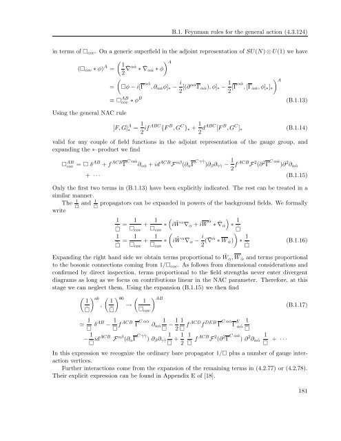
B.1. Feynman rules for the general action (4.3.124)
in terms of cov. On a generic superfield in the adjoint representation of SU(N) ⊗ U(1) we have
A 1
(cov ∗ φ) A =
=
2 ¯ ∇ α ˙α ∗ ¯ ∇α ˙α ∗ φ
φ − i[Γ α ˙α ,∂α ˙αφ]∗ − i
2 [(∂α ˙α Γα ˙α),φ]∗ − 1
2 [Γα ˙α ,[Γα ˙α,φ]∗]∗
≡ AB
cov ∗ φ B
Using the general NAC rule
[F,G] A ∗
= 1
2 ifABC {F B ,G C }∗ + 1
2 dABC [F B ,G C ]∗
A
(B.1.13)
(B.1.14)
valid for any couple of field functions in the adjoint representation of the gauge group, and
expanding the ∗–product we find
AB
cov = δAB + f ACB Γ C α ˙α ∂α ˙α + id ACB F αβ (∂αΓ C γ ˙γ )∂β∂γ ˙γ − 1
2 fACB F 2 (∂ 2 Γ C α ˙α )∂ 2 ∂α ˙α
+ · · · (B.1.15)
Only the first two terms in (B.1.13) have been explicitly indicated. The rest can be treated in a
similar manner.
The 1 ˆ and 1 e propagators can be expanded in powers of the background fields. We formally
write
1
ˆ
1
= +
cov
1
cov
1 1
= +
cov
1
∗
cov
∗
i ˜ W α ∇α + iW ˙α ∗ ¯ ∇ ˙α
∗ 1
ˆ
i ˜ W α ∇α − i
2 ( ¯ ∇ ˙α
∗ W ˙α) ∗ 1
(B.1.16)
Expanding the right hand side we obtain terms proportional to ˜ Wα,W ˙α and terms proportional
to the bosonic connections coming from 1/cov. As follows from dimensional considerations and
confirmed by direct inspection, terms proportional to the field strengths never enter divergent
diagrams as long as we focus on contributions linear in the NAC parameter. Therefore, at this
stage we can neglect them. Using the expansion (B.1.15) we then find
ab 00 AB 1 1 1
, →
ˆ cov
≃ 1
δAB − 1
fACB Γ C α ˙α 1 1 1
∂α ˙α −
2 fACDf DEB Γ C α ˙α Γ E 1
α ˙α
− 1
idACB F αβ (∂αΓ C γ ˙γ 1 1 1
) ∂β∂γ ˙γ +
2 fACB F 2 (∂ 2 Γ C α ˙α ) ∂ 2 1
∂α ˙α
+ · · ·
(B.1.17)
In this expression we recognize the ordinary bare propagator 1/ plus a number of gauge interaction
vertices.
Further interactions come from the expansion of the remaining terms in (4.2.77) or (4.2.78).
Their explicit expression can be found in Appendix E of [18].
181