Perturbative and non-perturbative infrared behavior of ...

4. Gauge theories
By direct calculation it turns out that diagrams (4.7d) and (4.7e) cancel one against the other
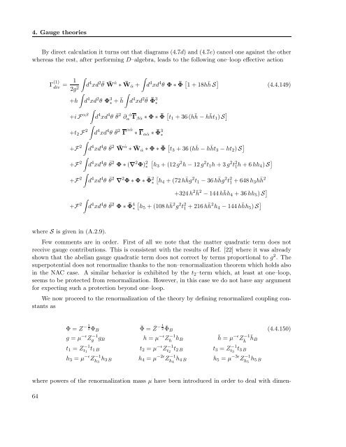
whereas the rest, after performing D–algebra, leads to the following one–loop effective action
Γ (1)
div
1
=
2g2
d 4 xd 2¯ θ ¯W ˙α
∗ ¯W ˙α + d 4 xd 4 θ Φ ∗ ¯Φ 1 + 18h¯ h S
(4.4.149)
+h d 4 xd 2 θ Φ 3 ∗ + ¯
h d 4 xd 2¯ θ ¯Φ 3 ∗
+i F αβ
d 4 xd 4 θ ¯ θ 2 ∂ ˙α
α Γβ ˙α ∗ Φ ∗ ¯Φ t1 + 36(h¯ h − h¯ ht1) S
+t2 F 2
d 4 xd 4 θ ¯ θ 2 Γ α ˙α ∗ Γα ˙α ∗ ¯Φ 3 ∗
+F 2
d 4 xd 4 θ ¯ θ 2 ¯W ˙α ∗ ¯W ˙α ∗ Φ ∗ ¯Φ t3 + 36(h¯ h − h¯ ht3 − ht2) S
+F 2
d 4 xd 4 θ ¯ θ 2 Φ ∗ (∇ 2 Φ) 2
∗ h3 + (12g 2 h − 12g 2 t1h + 3g 2 t 2 1h + 6hh4) S
+F 2
h4 + (72h¯ hg 2 t1 − 36h¯ hg 2 t 2 1 + 648h3h¯ h 2
d 4 xd 4 θ ¯ θ 2 ∇ 2 Φ ∗ Φ ∗ ¯Φ 2 ∗
+324h 2¯2 h − 144hhh4 ¯ + 36hh5) S
+F 2
d 4 xd 4 θ ¯ θ 2 Φ ∗ ¯Φ 4
∗ h5 + (108h¯ h 2 g 2 t 2 1 + 216h¯ h 2 h4 − 144h¯ hh5) S
where S is given in (A.2.9).
Few comments are in order. First of all we note that the matter quadratic term does not
receive gauge contributions. This is consistent with the results of Ref. [22] where it was already
shown that the abelian gauge quadratic term does not correct by terms proportional to g 2 . The
superpotential does not renormalize thanks to the non–renormalization theorem which holds also
in the NAC case. A similar behavior is exhibited by the t2–term which, at least at one–loop,
seems to be protected from renormalization. However, in this case we do not have any argument
for expecting such a protection beyond one–loop.
We now proceed to the renormalization of the theory by defining renormalized coupling constants
as
Φ = Z −1
2ΦB
¯Φ = ¯ Z −1
2 ¯ ΦB
g = µ −ǫ Z −1
g gB h = µ −ǫ Z −1
h hB
t1 = Z −1
t1 t1 B
h3 = µ −ǫ Z −1
h3 h3 B
t2 = µ −ǫ Z −1
t2 t2 B
h4 = µ −2ǫ Z −1
h4 h4 B
¯h = µ −ǫ Z −1
¯h ¯ hB
t3 = Z −1
t3 t3 B
h5 = µ −3ǫ Z −1
h5 h5 B
(4.4.150)
where powers of the renormalization mass µ have been introduced in order to deal with dimen-
64