Adaptive Predictive Regulatory Control with BrainWave - Courses ...

to be handled. For these reasons predictive control can remedy some of the
drawbacks associated with fixed gain controllers.
Based on an original theoretical development by Dumont et al. [5, 13, 14] the
controller was first developed for self-regulating systems. This controller was
credited by various users with several features among which we can mention:
the reduced effort required to obtain accurate process models, the inclusion of
adaptive feedforward compensation, the ability to cope with severe changes in
the process etc.
These features together with a recognized need in industry created the opportunity
for further development of a controller capable of dealing with integrating
systems with delay in the presence of unknown output disturbances.
These investigations lead to an indirect adaptive controller based on identification
using an orthonormal series representation working on-line in conjunction
with a predictive controller.
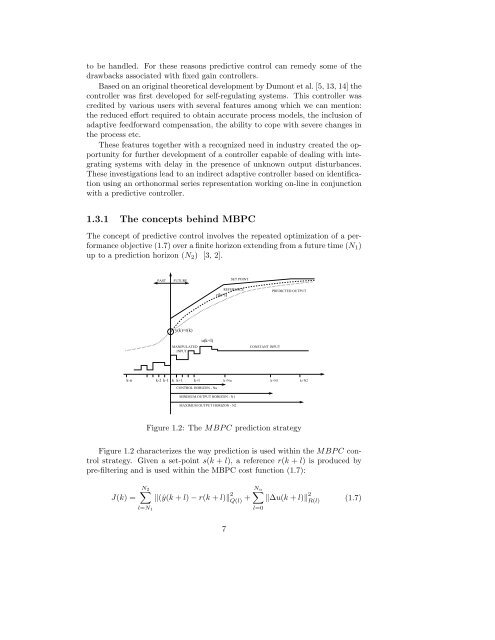
1.3.1 The concepts behind MBPC
The concept of predictive control involves the repeated optimization of a performance
objective (1.7) over a finite horizon extending from a future time (N1)
up to a prediction horizon (N2) [3, 2].
PAST FUTURE
y(k)=r(k)
MANIPULATED
INPUT
k-n k-2 k-1 k k+1 k+l
u(k+l)
SET POINT
REFERENCE
r(k+l)
CONTROL HORIZON - Nu
MINIMUM OUTPUT HORIZON - N1
MAXIMUM OUTPUT HORIZON - N2
CONSTANT INPUT
PREDICTED OUTPUT
k+Nu k+N1 k+N2
Figure 1.2: The MBPC prediction strategy
Figure 1.2 characterizes the way prediction is used within the MBPC control
strategy. Given a set-point s(k + l), a reference r(k + l) is produced by
pre-filtering and is used within the MBPC cost function (1.7):
J(k) =
N2
l=N1
(ˆy(k + l) − r(k + l) 2
Q(l) +
Nu
7
l=0
∆u(k + l) 2
R(l)
(1.7)