Download Full Paper - Sathyabama University

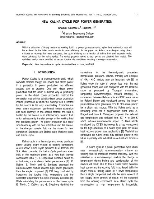
National Journal on Advances in Building Sciences and Mechanics, Vol. 1, No.2, October 2010 17
Abstract
NEW KALINA CYCLE FOR POWER GENERATION
Shankar Ganesh N. 1 , Srinivas T. 2
1,2
Kingston Engineering College
Email:nshankar_g@rediffmail.com
With the utilisation of binary mixture as working fluid in a power generation cycle, higher heat conversion rate will
be achieved in the boiler which results in more efficiency. In this paper two kalina cycle designs using binary
mixtures as working fluid were compared, the cycle efficiency as a function of turbine inlet and separator outlet
were calculated for the kalina cycles. The cycles property values at each points are obtained from matlab. The
optimized design were identified at various turbine inlet conditions resulting in energy conservation.
Keywords: New thermodynamic cycle, Ammonia-Water mixture, MATLAB
I. INTRODUCTION
Power Cycles is a thermodynamic cycle which
converts thermal energy into power and stores power
in a generator. In power production two different
aspects are in practice. One with direct power
production and the other is indirect way of producing
power. In the direct power production method the
conversion method that exhibits direct power production
include processes in which the working fluid is heated
by the source is the only intermediary. Examples are
solar steam expansion, geothermal steam expansion
and solar chimney. In the second method, the fluid is
heated by the source is an intermediary transfer fluid,
which subsequently transfer energy to the working fluid
that produces power. The power production can occur
simultaneously with the heat extraction from the source,
or the charged transfer fluid can be stores for later
generation. Examples are Stirling cycle, Rankine cycle,
and Kalina cycle.
Kalina cycle is a thermodynamic cycle, produces
power utilizing binary mixture as working component.
A well known Kalina Cycle produces O.M. Ibrahim and
S.A. Klein concluded the kalina Cycle produces about
80% of the maximum power at a very high thermal
capacitance ratio [1]. T.Heppenstall identified Kalina as
a bottoming cycle shows better performance [2]. C.
Dejfors, E. Thorin and G. Svedberg proposed the
ammonia-water mixture reaches high power generation
than the single component [3]. P.K. Nag concluded by
increasing the turbine inlet temperature and the
separator temperature the cycle efficiency increases [4].
While calculating the performance of the power cycle
E. Thorin, C. Dejfors, and G. Svedberg identified the
correlations for the thermodynamic properties
(temperature, pressure, volume, enthalpy and entropy)
of NH3 H2O mixture play an important role [5]. In
Kalina cycle the ratio of exergy loss with the net
generated power was less compared with the Rankine
cycle as proposed by Thongcai srinophakun,
sangapong Laowithavangkul, Masaru Ishida[6]. A
comparison between Kalina cycle and ORC were made
by Roland Dippio and concluded among the binary
plants Kalina cycle generates 30% to 50% more power
for a given heat source. With the Kalina cycle as a
bottoming cycle for a cogeneration plant Jose A.
Borgert and Jose A. Velasquez proposed the exhaust
gas temperature was reduced from 427 K to 350 K
which reduces environmental impact [7]. Mark Mirolli
concluded the DCSS technology is a key component
for the high efficiency of a Kalina cycle plant for waste
heat recovery power plant applications [8]. VasileMinea
conceived the Kalina cycle may produce power in the
future especially with industrial waste heat and biomass
[9].
A Kalina cycle is a power generation cycle which
uses non-azeotropic (ammonia-water) mixture as
working fluid for increased thermal efficiency. With the
utilization of a non-azeotropic mixture the change in
temperature during boiling and condensation of the
mixture will result. Due to this a closer match between
heat source and the working fluid is achieved. With the
binary mixture, boiling exists at a lower temperature
than a single component and with the same amount of
fuel supply more amount of steam will be extracted
from the working component. In a steam cycle the
condensation at high temperature is impossible.

18 National Journal on Advances in Building Sciences and Mechanics, Vol. 1, No.2, October 2010
Whereas in Kalina cycle the condensation at high
temperature and low pressure is achieved by the
incorporation of separator. With the utilization of binary
mixture the following improvements can be achieved.
(i) Reduction in fuel proportion with the gains in
efficiency.
(ii) For condensation low pressure is sufficient.
(iii) For spinning the turbine high pressure is
obtained.
Why Kalina Cycle?
In Rankine cycle more than half of the heat
transfer occurs during the boiling process
which is considered as constant temperature
boiling process.
In ORC utilizing isopentene as working fluid,
isopentene boils at a constant temperature
under a given pressure.
In Organic Rankine cycle the theoretical
efficiency and cost/production ratio are less.
Present work calculates the efficiency of the
existing real time cycle (Hawaii Plant) using MATLAB.
The practical efficiency calculation was compared with
the simulated value and happened to find a percentage
error of less than 5%. In addition to which a high
temperature plant was considered and the same
practical and simulated efficiencies were compared.
In addition, a new model is proposed and the
efficiency calculation were made.
II. CORRELATIONS FOR CALCULATING
THEMODYNAMIC PROPERTIES
For determining the performance of the power
cycle correlations the thermodynamic properties were
calculated. In this work the correlations proposed by
Ziegler and Trepp, Patek and Klomfar and Soleimani
were utilised and developed in MATLAB. The Gibbs
free energy for both liquid and vapor phases were used
for determining enthalpy, entropy and volume. The
correlations were coded in MATLAB and executed.
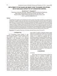
Hawaii Plant
The largest “waste heat” resource available in
Hawaii for kalina cycle application is the heat stores in
the tropical region surrounding the state.
The 10000 kW hawaii plant has inlet temperature
of 26C.
The process uses a binary working fluid of
ammonia and water with distillation / condensation
subsystem which enables different working fluid
mixtures at different stages of the cycle with heat
recuperative stages for increased efficiency.
The DCSS provides essential to the existence in
establishing the high ammonia-water concentration for
the heat acquisition stage and a low ammonia-water
concentration at the condensation stage.
Fig. 1. Hawaii Kalina Cycle Power Plant
Table 1 Plant Performance Summary
Plant Simulation
Heat In 513897.50 kW 513897.50 kW
Heat Rejected 503729.64kW 503729.64kW
Power Turbine 10526.32 kW 10048.34 kW
Gross Generator
Power
10105.26 kW 9646.40 kW
Power Pumps 382.25 kW 427.96 kW
Net Output 10144.07 kW 10476.3 kW
Thermal
Efficiency
1.97% 2.02%
Plant Efficiency 1.54% 1.46%

N. Shankar Ganesh et al : New Kalina Cycle for Power ...
Table 2. Comparative state point values of Hawaii plant with the simulated results
Point X Plant X
Simulation
T Plant T
Simulation
P Plant P Sim. H Plant H Sim. Mass
Plant
Mass
Sim.
9 0.68 0.69 22.95 23 5.887 5.919 103 97.57 600.41 647.35
10 0.68 0.69 22.79 22.83 5.852 5.88 103 98.31 600.41 647.35
12 0.68 0.69 17.88 17.33 5.576 5.86 127.78 118.79 600.41 647.35
13 0.68 0.69 14.64 17.16 4.42 4.5 127.78 118.79 600.41 647.35
14 0.802 0.802 6.78 7 4.353 4.39 114.65 111.15 967 1013.9
23 Brine Brine 4 4 16.75 15.75 16862.95 16862.95
24 Brine Brine 11.13 11.13 16.62 16.62 16862.95 16862.95
25 Brine Brine 26 26 103.9 103.9 16773.04 16773.04
26 Brine Brine 18.33 18.33 73.27 73.27 16773.04 16773.04
29 0.802 0.802 14.45 14.13 4.42 4.54 406.27 396.68 967 1013.9
30 0.9998 0.9998 22.88 23 5.861 5.86 1309.68 1312. 1 366.59 366.59
31 0.9998 0.9998 8.11 10 4.444 4.44 1280.97 1284.7 366.59 366.59
32 0.9998 0.9998 8.03 9.9 4.42 4.39 1280.97 1284.7 366.59 366.59
33 0.802 0.802 14.45 14.13 4.42 4.39 406.27 388.65 967 1013.9
36 0.802 0.802 6.78 7 4.353 4.39 114.65 111.15 967 1013.9
37 0.802 0.802 6.82 7 6.466 5.91 114.28 110.63 967 1013.9
38 0.802 0.802 6.82 7 6.466 5.91 114.28 110.63 967 1013.9
39 0.802 0.802 6.83 7.007 6.1 5.83 114.28 110.63 967 1013.9
40 0.802 0.802 6.83 7.007 6.1 5.83 114.28 110.63 967 1013.9
41 0.802 0.802 6.83 7.007 6.059 5.83 114.28 110.63 934.3 983.95
43 0.802 0.802 23.22 23 5.92 5.77 435.86 411.51 934.3 983.95
44 0.802 0.802 6.83 7.007 6.059 5.83 114.28 110.63 32.86 29.98
46 0.802 0.802 20.56 20 5.92 5.77 325.77 409.61 32.86 29.98
47 0.802 0.802 22.95 20 5.887 5.77 432.11 409.61 967 1013.9
48 0.802 0.802 22.95 23 5.887 5.91 432.11 478.42 967 1013.9
49 0.9998 0.9998 22.95 23 5.887 5.91 1309.68 1311.5 366.59 366.59
50 0.9998 0.9998 22.93 22.77 5.877 5.86 1309.68 1310.6 366.59 366.59
51 0.9998 0.9998 22.91 22.54 5.872 5.80 1309.68 1310.6 366.59 366.59
52 0.9998 0.9998 22.88 23 5.861 5.86 1309.68 1310.6 366.59 366.59
19

20 National Journal on Advances in Building Sciences and Mechanics, Vol. 1, No.2, October 2010
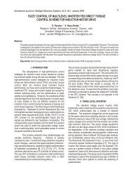
III. THERMODYNAMIC CYCLE
The working fluid ammonia-water mixture is
vaporized and superheated in the HRVG before
expansion through the turbine. The relatively high
concentration of ammonia in the working fluid is called
the working mixture composition. The superheated
vapor (11) is then expanded in the turbine (12) to
transform its energy into useful form. The generated
spent stream is then cooled in a distiller (13) and
diluted (5) with a weak solution resulting in basic
mixture composition (14). The basic mixture
composition raises the condensing temperature and
condensed in the absorber. A stream with a high
concentration of ammonia, like the turbine outlet
stream, cannot be condensed by cooling water of a
normal temperature, since the high ammonia
concentration would result in a very low condensation
temperature at the pressure level in the condenser. A
pump (15) increases the pressure of the basic mixture
Fig. 2. Schematic diagram of Kalina Cycle
Working Mixture
Ammonia lean solution
Basic Mixture
Ammonia rich vapour
CDP = Condensate Pump
BFP = Boiler Feed Pump
HRVG = Heat Recovery
Vapour Generator
condensate and the stream is split: one (17) of the
resulting streams is sent to the separator via the
reheater and the other stream (18) is mixed with the
ammonia-rich vapor from the separator to restore the
working mixture concentration. One of the resulting
streams (1) is sent is sent to the separator via the
reheater recovering heat from the turbine outlet stream.
The flash tank separator produces one stream of
ammonia-lean saturated liquid (3) and one stream of
ammonia-rich saturated vapor (2). The ammonia-lean
liquid stream gives up heat in the reheater , then
throttled (5)and absorbs the working mixture stream
(14) from the turbine before condensation in the
low-pressure condenser. The other stream (18) is
mixed with the ammonia-rich vapor (6) from the
separator to restore the working mixture concentration
(7). Then it is condensed in a condenser (8),
pressurized in a boiler feed pump (9) and sent into the

N. Shankar Ganesh et al: New Kalina Cycle for Power ...
HRVG where it is superheated by the source. The real
focus of any power cycle is to increase the cycle
efficiency by reducing the structural losses. Reduction
in structural losses (Figure 2) results in increased
actual work. In a single component working fluid cycle
as the boiling and condensation temperature is
constant, therefore the working fluid curve is not
paralleled with the heat source curve.
Fig. 3. T-S plot of Kalina Cycle with heat source
IV. THERMODYNAMIC ANALYSIS
To carry out thermodynamic analysis Energy
balance, Mass balance and Material balance were to
be find out. The first step in calculating the performance
of the cycle is to perform mass balance and energy
balance. The equations for all the components were
made out.
SEPARATOR:
For the input parameters, pressure, concentration
and temperature using MATLAB the liquid concentration
X1 and Vapor concentration Xv was calculated.
TURBINE:
h11 h12 Th12 h11s where, s 12 s 11s
PUMP:
h16 h15 h15 h16 /p Where, s15 s16s h 9 h 8 h 8 h 9s / p Where, s 8 s 9s
For pump and turbine the efficiencies
were assumed as T 0.9 p 0.6
REHEATER:
m 3 h 3 h 4 m 19 h 19 h 17
In reheater, distiller, and feed water heater the
Terminal Temperature Difference was assumed as
5C to 10C
MIXER:
m5 h5 m13 h13 m14 h14 m 6 h 6 m 18 h 18 m 17 m 17
With these equations the enthalpy, Entropy and
volume values for all the Points considered in the cycle
was obtained using MATLAB. The thermodynamic
properties evaluated
using the correlations proposed were helpful in
obtaining the values at each points in a fast manner.
V. EFFICIENCY CALCULATION:
The efficiency of the cycle is the ratio of the
output with the input. The output is considered as the
turbine work and pumps work. The input is consided
at the HRVG.
TURBINE WORK:
Wt m11 h11 h12 BOILER PUMP WORK:
Pw1 v8 p8 p9m8 R T8 T9 21

22 National Journal on Advances in Building Sciences and Mechanics, Vol. 1, No.2, October 2010
Point P, bar TC
Existing
Table 2 Input Parameters
TC X Existing X obtainted H, kJ/kg
Existing
H, kJ/kg
obtained
S, kJ/kg K Z, kJ/kg K
Existing obtained
M, Kg
Existing
M, Kg
obtained
1 5.539 70 70 0.448 0.448 312 376 1.49 1.33 2.94 3.23
2 5.539 70 70 0.9685 0.979 1482 1450.95 5.2 4.75 0.48 0.47
3 5.539 70 70 0.3459 0.3568 82 93 0.76 0.69 2.46 2.75
4 5.539 25.06 25.05 0.3459 0.3568 117 114.8 0.14 0.0425 2.46 2.75
5 2 25.17 25 0.3459 0.3568 117 114.8 0.14 0.04 2.46 2.75
6 5.539 27.36 27 0.9685 0.979 1316 1283.88 4.7 4.22 0.48 0.47
7 5.539 42.92 39 0.7 0.7 557 603 2.3 1.84 1.00 1.00
8 5.539 20 20 0.7 0.7 107 107 0.10 0.007 1.00 1.00
9 100 23.56 22 0.7 0.7 80 87.6 0.13 0.02 1.00 1.00
10 100 39.09 42 0.7 0.7 0.007 0.409 0.40 0.32 1.00 1.00
11 100 500 500 0.7 0.7 2798 2799 6.27 6.208 1.00 1.00
12 2 118.87 113 0.7 0.7 1897 1888 6.52 5.45 1.00 1.00
13 2 57.47 59 0.7 0.7 1041 1198 4.0 3.559 1.00 1.00
14 2 40.15 39 0.448 0.7 209 234 1.27 0.97 3.46 3.75
15 2 20 20 0.448 0.448 154 156 0.043 0.068 3.46 3.75
16 5.539 20.06 20.05 0.448 0.448 154 155.9 0.044 0.068 3.46 3.75
17 5.539 20.06 20.05 0.448 0.448 154 155.9 0.044 0.068 0.51 0.52
18 5.539 20.06 20.05 0.0448 0.448 154 155.9 0.044 0.068 0.51 0.52
19 5.539 52.47 54 0.448 0.448 12 28 0.58 0.42 2.94 3.23
20 5.539 70 70 0.448 0.448 312 376 1.49 1.33 2.94 3.23
CONDENSATE PUMP WORK:
HRVG:
P w2 v 15 p 15 p 16m 15 R T 15 T 16
Qs m 11 h 11 h 10
EFFICIENCY:
W t Pw 1 Pw 2
Qs
With this calculation the efficiency of the cycle
was obtained.
VI. RESULTS AND DISCUSSIONS:
Table 1 gives the values of the cycle nodes
chosen. The poperty values as well as the mass and
energy values. The values obtained were calculated
using the proposed correlations in MATLAB. The values
obtained by the present result are comparibly closer
with the existing results with deviations upto 2% to 5%.
The important parameters which affect the cycle
efficiency was assessed as turbine inlet temperature,
separator temperature and turbine inlet concentration.
The effeciencies at various separator temperature and
turbine inlet concentration were calculated and plotted.
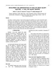
Figure 3 shows the cycle efficiency graph as a function
of separator temperature and turbine inlet concentration

N. Shankar Ganesh et al: New Kalina Cycle for Power ...
with the constant turbine inlet temperature. At constant
turbine inlet temperature, the separator temperature
decreases with the increase in the turbine inlet
concentration. The cycle efficiency as a function of
turbine inlet temperature and inlet concentration is
shown in the figure 4 the turbine inlet temperature inlet
concentration.
Fig. 4 Cycle efficiency as a function of separator
temperature and turbine inlet Concentration
Fig. 5 Cycle efficiency as a function of Turbine Inlet
temperature and turbine inlet Concentration
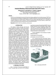
A. NEW KALINA CYCLE APPLICABLE FOR LOW
PRESSURE APPLICATIONS
WORKING PRINCIPLE:
The cycle shown in the figure.5 is suitable for
low pressure applications. The cycle shown is used for
converting energy from low pressure, moderate
temperature stream (external source) into usable
energy by a binary mixture working component. The
cycle consists of high pressure circuit and low pressure
circuit. The present cycle involves eight heat
exchangers, a separator, a turbine, two pumps, a mixer
and a separator. In this cycle the irreversibility in the
process of mixing the basic solution with the
re-circulating solution was reduced by vaporizing the
basic solution completely and preheating the
re-circulating before mixing which reduces the
irreversibility in the process of mixing and increases
the efficiency of the overall process. Also the flow rate
of the working solution passing through the turbine will
be increased, thus an increased power output. Initially
the basic solution is pumped in a pump (P1) and
pressurised which then is heated in a recuperative
preheater by condensed basic solution. During the first
heat exchange process and during the preheated
steam and condensed steam will be produced. The
preheated steam at a state of saturated state is splitted
into two streams, one of the two streams is passed in
a heat exchanger where it is partially vaporized by the
counter flow
heat source fluid stream and considered as
second heat exchange process. The other stream is
partially vaporized by the condensing working fluid
stream . The two partially vaporized streams are
combined at a state of liquid-vapor mixture. The mixture
is further heated and vaporized with the cooled heat
source in a fourth heat exchange process resulting in
a state of saturated vapor.The working solution stream
is then heated and vaporized with a first cooled heat
source fluid stream in a fifth heat exchange process
producing saturated vapor. The vapor is heated in heat
exchanger producing superheated vapor which is then
expanded in a turbine. The spent stream is used to
heat the preheated stream in the recuperative
preheater.
Fig. 6 New Kalina Cycle Applicable for Low
Pressure Applications
T = Turbine
SHT = Super Heater
EPR = Evaporator
HE = H eat Exchang er
EM R = Economiser
RBC = Recuperative
Boiler -Condenser
SPR = Separator
R PH = R ecuperative
Preheater
P = Pum p
S = Splitter
M = Mixer
23

24 National Journal on Advances in Building Sciences and Mechanics, Vol. 1, No.2, October 2010
Table 3 Property values of the at cycle points
Point X T (C) P, (bar) h, (kJ/kg) s, (kJ/kg-K) m, (kg)
1 0.8245 77 8.25 1070 3.89 1.17
2 0.952 77 8.25 1440 4.67 0.87
3 0.385 77 8.25 127 0.77 0.29
4 0.385 77 8.25 127 0.77 0.17
5 0.385 77 8.25 127 0.77 0.12
6 0.9 77 8.25 1280 4.3 1
7 0.9 45 8.10 966 3.12 1
8 0.9 21 8.09 20.54 0.237 1
9 0.9 21 32.65 22.72 0.24 1
10 0.9 73.9 31.99 283.37 1.04 1
11 0.9 72 31.99 283.37 1.04 0.60
12 0.9 73.9 31.99 283.37 1.04 0.40
13 0.9 104 31.87 1284 4.26 0.60
14 0.9 104 31.87 1284 4.26 0.40
15 0.9 104 31.87 1284 4.26 1
16 0.9 142 31.87 1632 4.70 1
17 0.8245 142 31.87 1454 4.40 1.17
18 0.8245 160 31.74 1758 4.95 1.17
19 0.8245 183 31.70 1826 5.0 1.17
20 0.8245 109 8.49 1582 4.75 1.17
21 0.385 77 31.99 127 0.7 0.17
22 0.385 142 31.87 478.7 1.77 0.17
31 0.385 77 31.99 127 0.7 0.17
40 187 1.013 786 2.26 2.58
41 179 1.013 723.83 2.05 2.58
42 147 1.013 615.04 1.59 2.58
43 147 1.013 615.04 0.90 0.18
44 109 1.013 343 1.68 0.18
45 109 1.013 500 1.65 2.40
46 147 1.013 615.04 0.98 2.40
47 82 1.013 343 1.10 0.18
48 77 1.013 319 1.04 2.58

N. Shankar Ganesh et al: New Kalina Cycle for Power ...
Fig. 7. T-S Plot of the proposed model
Fig. 8. T-H Plot of the proposed model
Table. 2 shows the property values at all cycle
points chosen. Based on the energy and mass balance
equation as calculated for the above cycle, the property
values at each cycle points were calculated. The
efficiency of the cycle is then calculated.
Figure 9 shows the cycle efficiency plot with the
constant parameter turbine inlet temperature, variable
separator temperature and turbine inlet concentration.
The trends shows that the cycle efficiency decreases
at increased concentration.The trends were obtained
with the parameters identified in affecting the efficiency
of the cycle. At constant Turbine inlet temperature and
at various separator temperatures the cycle efficiency
were calculated. Also the cycle efficiency were
calculated by considering constant separator
temperature and varied turbine inlet temperature.
VII. CONCLUSION
The main goal of this work is to extract more
energy from the heat source and efficiently converted
to work output. The basic cycle was considered and
using MATLAB the properties were calculated as the
preliminary measure. The efficiency was calculated and
compared with the existing results. With the new cycle
applicable for moderate temperature and low pressure
applications will utilize the heat source much more
efficiently as the recirculating solution is combined with
the working solution which in turn increases the heat
load with a high flow rate in the turbine inlet. With the
utilization of multiple heat exchangers the complete
vaporization in the super heater and complete
condensation in the condenser is achieved.
Fig. 9 New Kalina Cycle Applicable for Low
Pressure Applications
Nomenclature
m mass flow
h specific enthalpy, kJ/kg
s specific entropy, kJ/kg-K
v specific volume, m 3 /kmol
T temperature, K
p pressure, bar
W Power
P Pump
cycle efficiency
R Gas Universal Constant
Subscripts
t turbine
25

26 National Journal on Advances in Building Sciences and Mechanics, Vol. 1, No.2, October 2010
REFERENCES
[1] Ibrahim O.M. and Klein S.A .(1996). “Absorption Power
Cycles”, Energy (1), pp. 21-27B.
[2] Heppenstall T. (1998). “Advanced Gas Turbine Cycles
for Power Generation a Critical Review”, Applied
Thermal Engineering (18) pp. 837-846.
[3] Dejfors C., Thorin E., and Svedberg G. [199].
“Ammonia-Water Power Cycles for Direct-Fired
Cogeneration Applications” (16) pp.1675 – 1681.
[4] Nag P.K. and Gupta A.V.S.S. (1998) “Exergy Analysis
of Kalina Cycle”, Applied Thermal Engineering (18)
pp.427-439.
[5] Thongchai Srinophakun, Sangapong Laowithayangkul,
Masaru Ishida (2001) “Simulation of Power Cycle with
Energy Utilization Diagram” Energy Conversion and
management” pp.1437-1456.
[6] Ronald DiPippo (2004). “Second Law assessment of
binary plants generating power from low-temperature
geothermal fluids”, Geothermics (33) pp. 565-586.
[7] Jose A. Borgert and Jose A.Velasquez (2004).
“Exergoeconomic Optimization of a Kalina Cycle for
Power Generation” Int.J.Exergy Vol.1.No.1.
[8] Mark D.Mirolli (2005). “The Kalina cycle for Cement
Kiln Waste Heat Recovery Power Plants” IEEE.
[9] Vasile Minea (2007). “Using Geothermal Energy and
Industrial Waste Heat for Power Generation” IEEE.
[10] Srinivas (2008). “Generalised Thermodynamic Analysis
of Steam Power Cycles with ‘n’ number of feed water
heaters”Int.J. of Thermodynamics (4), pp. 177-185.