measurement and comparison of solar radiation estimation models ...

More documents

Recommendations

Info

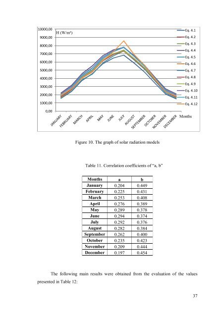
10000,00 H (W/m²) Eq. 4.1 9000,00 Eq. 4.2 8000,00 7000,00 6000,00 5000,00 4000,00 3000,00 2000,00 1000,00 0,00 Figure 10. The graph of solar radiation models Table 11. Correlation coefficients of “a, b” Months a b January 0.204 0.449 February 0.225 0.431 March 0.253 0.408 April 0.276 0.389 May 0.289 0.378 June 0.294 0.374 July 0.292 0.376 August 0.282 0.384 September 0.262 0.400 October 0.235 0.423 November 0.209 0.444 December 0.197 0.454 The following main results were obtained from the evaluation of the values presented in Table 12: Eq. 4.3 Eq. 4.4 Eq. 4.5 Eq. 4.6 Eq. 4.7 Eq. 4.8 Eq. 4.9 Eq. 4.10 Eq. 4.11 Eq. 4.12 Months 37
Evaluation of Group 1: There is only one equation in this group. The results for MBE = -595.294 W/h, RMSE = 685.838 W/h, t-stat=5.797 and e=-12.727 were obtained from Eq. 4.1. Evaluation of Group 2: There are two equations in this section. They were Eqs. 4.7 and 4.10. The best results for MBE = -10.324 W/h, t-stat=0.100 and e=-0.2207 were obtained from Eq. 4.10 and best results for RMSE = 325.248 W/h from Eq. 4.7. Evaluation of Group 3: Six models were compared in this part. The best results for MBE = -0.968 W/h, RMSE = 337.305 W/h, t-stat=0.010 and e=-0.0207 were obtained from the new developed model Eq. 4.11. Evaluation of Group 4: There were also two models in this group. The best results for MBE = 1.112 W/h, t-stat=0.007 and e=0.02377 were obtained from the new developed Eq. 4.12 and the best result RMSE = 440.037 W/h was obtained from Eq. 4.8. Among the solar radiation models, for all test methods, the author’s model given by Eq. (4.14) was found to be the most accurate model, followed by Eq. (4.13) and Eq. (4.12) respectively. By looking at the relative percentage errors, it has seen that the new developed models gave the closest values rather than the other models. They were followed by Eq. (4.9) and Eq. (4.7). Table 12. Comparison of statistical methods for global solar radiation models Method Model MBE ( W/m²) RMSE ( W/m²) t-stat e% 1 -595,294 685,838 5,797 -12,727 2 -213,304 409,644 2,023 -4,5603 3 -202,884 406,316 1,911 -4,3375 4 225,261 350,564 2,781 4,81593 5 -409,445 575,035 3,363 -8,7537 6 -222,139 417,388 2,085 -4,7492 7 113,374 325,248 1,233 2,42385 8 -260,684 440,037 2,439 -5,5733 9 -158,001 365,375 1,591 -3,378 10 -10,324 343,676 0,100 -0,2207 11 -0,968 337,305 0,010 -0,0207 12 1,112 530,150 0,007 0,02377 38
Page 1 and 2: MEASUREMENT AND COMPARISON OF SOLAR
Page 3 and 4: ACKNOWLEDGEMENTS First of all, the
Page 5 and 6: ÖZET İZMİR/TÜRKİYE İÇİN GÜ
Page 7 and 8: 4.8. Ulgen and Hepbasli’s Model
Page 9 and 10: Table LIST OF TABLES Table 1. Turke
Page 11 and 12: DMI EIEI IYTE MBE RMSE e t-stat MPE
Page 13 and 14: development. Globally, an estimated
Page 15 and 16: eceived directly (direct radiation)
Page 17 and 18: According to these data, Turkey's a
Page 19 and 20: 2.1. Global Solar Radiation CHAPTER
Page 21 and 22: Electrical Works Research Directora
Page 23 and 24: Togrul et al. (2002) developed some
Page 25 and 26: so widely throughout China that the
Page 27 and 28: Figure 2. Approximate construction
Page 29 and 30: Meteorological data including tempe
Page 31 and 32: CHAPTER 4 ANALYSIS OF GLOBAL RADIAT
Page 33 and 34: The equation was in the Group 2. H
Page 35 and 36: CHAPTER 5 ANALYSIS OF DIFFUSE RADIA
Page 37 and 38: 5.3. 퐇 퐝 as a Function of 퐇
Page 39 and 40: CHAPTER 6 RESULTS 6.1. Results for
Page 41 and 42: Table 5. Hₒ values for Izmir Mont
Page 43 and 44: 1000 900 800 700 600 500 400 300 20
Page 45 and 46: According to Table 9 the maximum va
Page 47: 36 Table 10. Hourly average global
Page 51 and 52: 2000 1800 1600 1400 1200 1000 800 6
Page 53 and 54: The following main results were obt
Page 55 and 56: CHAPTER 7 CONCLUSION In this thesis
Page 57 and 58: Haydar A.; Balli O.; Hepbasli A. (2
Page 59 and 60: Yildiz, M. and Oz, S. (1994), Evalu
Page 61 and 62: 700 600 500 400 300 200 100 0 900 8
Page 63 and 64: 800 700 600 500 400 300 200 100 0 6

measurement and comparison of solar radiation estimation models ...

You also want an ePaper? Increase the reach of your titles

Delete template?

Save as template?