Movable cellular automata method for simulating materials with ...

Movable cellular automata method for simulating materials 

with mesostructure 

S.G. Psakhie a,* , Y. Horie b , G.P. Ostermeyer c , S.Yu. Korostelev a , 

A.Yu. Smolin a , E.V. Shilko a , A.I. Dmitriev a , S. Blatnik e ,M.Spegel d , 

S. Zavsek f 

a Institute of Strength Physics and Materials Science, Russian Academy of Sciences, pr. Academicheskii 2/1, Tomsk 634021, Russia 

b Los Alamos National Laboratory, MS D413, X-MH, Los Alamos, NM 87545, USA 

c University of Braunschweig, Institute of Engineering Mechanics, Schleinitzstrasse 20, D-38106Braunschweig, Germany 

d Jozef Stefan Institute, Jamova 39, SI-1000 Ljubljana, Slovenia 

e IPAK, Koroska 18, SI-3320 Velenje, Slovenia 

f Velenje Coal Mine, Partizanska 78, SI-3320, Velenje, Slovenia 

Abstract 

Mathematical formalism and applications of the movable cellular automata MCA) method are presented for 

solving problems of physical mesomechanics. Since the MCA is a discrete approach, it has advantages over that of the 

®nite element method FEM). Simulation results agree closely with the experimental data. The MCA approach cab 

solves mechanical engineering problems ranging from those in material science to those in structures and constructions. 

Computer simulation using MCA can also provide useful information in situations where direct measurements are not 

possible. Ó 2001 Published by Elsevier Science Ltd. 

1. Introduction 

Theoretical and Applied Fracture Mechanics 37 2001) 311±334 

Mechanics is the science that treats motion. A 

Material to be described can be represented as a 

continuum or multitude of interacting particles. 

These approaches were suggested by Cauchy and 

Navier, in the early 19th century. The continuum 

approach prevailed for a long period of time. 

The development and elaboration of numerical 

methods were an important stage in the development 

of mechanics. It was associated with the 

* 

Corresponding author. Tel.: +7-382-2-258881; fax: +7-382-2- 

259576. 

E-mail addresses: sp@ms.tsc.ru, psakhie@yahoo.com S.G. 

Psakhie). 

0167-8442/01/$ - see front matter Ó 2001 Published by Elsevier Science Ltd. 

PII: S 0 1 6 7 - 8 4 4 2 0 1 ) 0 0 079-9 

www.elsevier.com/locate/tafmec 

advent of computer. Computational mechanics is 

considered to be an independent part of mechanics 

that supplements theoretical and experimental investigations; 

it is often referred to as computer 

experiments. 

Digitization has also improved accuracy of 

numerical solutions, particularly for solving the 

equations of continuum mechanics. Advances in 

computational mechanics cannot be overemphasized 

for its application to virtual testing and design. 

Discrete computational mechanics has been 

developed as Molecular Dynamics problems at the 

atomic level. However, the potentials of the discrete 

approach are by no means fully developed. 

The last 15±20 years have been marked by 

works where the particle method was used to de

312 S.G. Psakhie et al. / Theoretical and Applied Fracture Mechanics 37 2001) 311±334 

scribe di€erent media including granular and loose 

materials. These works can be found in [1±11]. In 

addition to the conventional Newton±Euler 

equations of motion, moment equations are also 

used. Particle interaction including atoms) considers 

the nearest neighbor with a time step integration 

of equations of motion [12,13]. While the 

adiabatic assumption has made those analyses 

meso- and macrolevels involve certain arti®cial 

expedients when integrating equations of motion. 

Thus, the models based on the conventional 

Newton±Euler addresses point masses, even 

though they include the moment equations. To 

overcome this contradiction, the method of movable 

cellular automata MCA) [14±16] was developed 

by the authors in the framework of joint 

projects. 

2. MCA method 

2.1. Basic approach 

Consider a system to be simulated by an ensemble 

of interacting automata elements) of ®nite 

size [16]. The concept of this method is based on 

the introduction of a new type of states, viz., the 

state of a pair of automata, into that of classical 

cellular automata. This has made possible a space 

variable that serves as a parameter of switching. 

The overlapping of a pair of automata was chosen 

as 

h ij ˆ r ij 

r ij 

0 ; …1† 

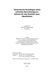
which is exhibited in Fig. 1a). The distance r ij 

between the centers of neighboring automata is 

shown in Fig. 1b) with d i being the automata size. 

For the simplest case, two states of pairs prevail: 

Linked state: h ij < h ij 

max ; …2† 

Unlinked state: h ij > h ij 

max : …3† 

The linked state is indicative of chemical bonds 

between elements and the unlinked state corresponds 

to the situation that there is no chemical 

bond between automata. Note that hij and rij are 

length parameters. They are capable of changing 

their positions in space and, consequently, changing 

the spatial arrangement of the entire system. 

The change in state of the automata pairs is governed 

by relative displacements of the automata 

pair. It follows from Eqs. 2) and 3) that the given 

medium constituted by such pairs can be considered 

as a bistable medium. 

Consider a pair of automata ij. The state of this 

pair of automata is uniquely determined by two 

types of ®elds hab…t†. The ®rst is associated with the 

state of the pair itself ij±hij…t† and the second is 

associated with the states of its neighboring pairs 

fikg±hik and fjlg±hjl . It is worthy of note that 

these ®elds de®ne local deformations deformation 

of elements of the medium) and, consequently, the 

distribution and ¯uxes of elastic energy in the 

simulated medium. 

The time derivative hij…t† can be determined 

following the Viner±Rothenblute model [17]. The 

active bistable medium under study can be described 

by the equation 

Dh ij 

Fig. 1. Pair of automata: a) overlapping state, b) contact state. 

Dt ˆ f …hij †‡ X 

C…ij; ik†I…h 

k6ˆj 

ik † 

‡ X 

C…ij; jl†I…h jl †; …4† 

l6î

S.G. Psakhie et al. / Theoretical and Applied Fracture Mechanics 37 2001) 311±334 313 

where the function f …hij † is indicative of the relative 

velocity of automata …V ij † and C…ij; ik…jl†† the 

coe cient associated with the transfer of the parameter 

h from the pair ik or jl) to the pair ij with 

I…hik…jl† † being an explicit function of hik…jl† . Here 

hik…jl† de®nes the redistribution of the parameters 

hik and hjl between the pairs ij, ik, and jl. These 

parameters are shown in Fig. 2. 

Within the linear approximation, the function 

I…hik…jl† † can be written as 

I…h ik…jl† †ˆw…aij;ik…jl††V i…k†…j…l†† 

n : …5† 

In general, the multiplier w…aij;ik…jl†† is a combination 

of trigonometrical functions and is de®ned by 

mutual arrangements of the automata ij, ik, and 

jl. Note that aij;ik…jl† is a set of values of the corresponding 

angles de®ned by the relative arrangement. 

The change in the overlapping parameter h ij for 

the pair ij is de®ned by the following factors: 

· relative velocity between the elements i and j 

V ij ); 

Fig. 2. Overlapping parameters for the pairs ij, ik, and jl. 

· change in the overlaps Dh ij ) of the ith automaton 

and its neighbors; 

· change in the overlaps Dh jl ) of the jth automaton 

and its neighbors. 

2.2. Motion of MCA 

It follows from Eq. 1) that the system consisting 

of movable cellular automata shall be described 

by the translational equations of motion 

given by 

d 2 h ij 

dt 

2 ˆ 

1 1 

‡ 

mi mj pij ‡ X 

C…ij; ik†w…aij;ik† 

k6ˆj 

1 

pik 

mi ‡ X 

C…ij; jl†w…aij;jl† 1 

mj pjl : …6† 

l6î 

To obtain Eq. 6), the term …d=dt†V i…j†k…l† was 

represented as …1=m i †p i…j†k…l† , where p i…j†k…l† is the 

force of inter-element interaction. It is de®ned by 

the function of the inter-automata response. The 

coe cient C…ij; ik…jl††, as stated in Eq. 4), is associated 

with the transfer of the parameter h from 

the pair ik or jl ) to the pair ij. The term w…aij;ik† in 

Eq. 5) is determined by the Poisson ratio and is 

related to the mutual arrangement of the pairs of 

elements ij and ik. 

The equations of motion for rotation can be 

written as 

d 2 h ij 

qij qji 

ˆ ‡ 

dt2 J i J j 

‡ X 

l6î 

s ij ‡ X 

k6ˆj 

S…ij; ik† qik 

sik 

J i 

S…ij; jl† qjl 

J j sjl : …7† 

Here, h ij is the angle of the relative rotation of 

elements switching parameter) similar to h ij ; q ij 

the distance from the center of the automaton i to 

the point of contact with the automaton j moment 

arm); s ij the tangential interaction of pairs; and 

S…ij; ik…jl†† the coe cients associated with the 

transfer of the parameter h from the pair ik or jl) 

to the pair ij. If C…ij; ik…jl†† ˆ 1 and 

S…ij; ik…jl†† ˆ 1, Eqs. 6) and 7) are completely 

equivalent to the Newton±Euler equations of 

motion for many-particle interaction.


As noted above, the term C…ij; ik…jl†† determines 

the transfer of the parameter h from the pair 

ik or jl) to the pair ij. The term `èlastic information'' 

implies information for relative elastic 

displacements of elements transferred to elastic 

®elds. Hence, equations of motion or Eqs. 6) and 

7) make it possible to allow for ``delays'' dt ij…ik† 

and dt ij…il† . This a€ects the overlapping parameter 

for the pairs {ik} and {jl} on the interaction of the 

pair of elements ij Fig. 2). The time lag is de®ned 

by the automata sizes, longitudinal and transverse 

sound velocities, and mutual arrangement of the 

pairs ij and ik or jl). It is obvious that the e€ects 

associated with generation and propagation of 

shock waves require particular attention. 

2.3. Volumetric changes 

For the method of embedded particles, Eqs. 

6)and 7) can be written as 

m i d2R i 

ˆ Fi 

dt2 X 

X 

‡ F ii ; j _i d 2~ i 

h X 

ˆ K 

dt2 ij ; …8† 

j 

where F i 

X is the volume-dependent force acting on 

the automaton i caused by the action of pressure 

from neighboring automata, F i ˆ pij ‡ sij . Here pij is the central component of the pair interaction 

force and sij the tangential component of this 

force. K ij ˆ qij…nij sij † is the unit vector nij de- 

®ned as n ij ˆ…R j R i †=…q ij ‡ q ji †. 

The volume-dependent force F i 

X acting on the 

automaton i due to the action of pressure from 

surroundings can be accounted for similar to the 

embedded atom method EAM) known from 

molecular dynamics [18]: 

F i 

X 

X 

ˆ P j S ij n ij : …9† 

j 

The index j …j ˆ 1; ...; N i † refers to automata in 

the linked state or the contact state with automaton 

i. It should be noted that P j is the pressure of 

the jth neighbor; S ij the area of contact of the 

automaton i with the automaton j; and n ij the unit 

vector of the normal to the contact area. Here n ij is 

directed towards the neighbor j. The automaton 

pressure is determined by the change in the auto- 

j 

mation volume. In the simplest linear) case this 

dependence takes the form 

P j ˆ K j Xj X j 

0 

X j 

0 

where X j 

0 

; …10† 

is the initial equilibrium) automaton 

volume; X j the current automaton volume; and K j 

the bulk modulus. The simplest approximation 

corresponds to the change in the automaton volume 

for a time Dt. It can be determined from the 

corresponding changes in the distances Dq jk from 

the center of this automaton to the points of its 

contact with neighbors, i.e., 

DX j j 

XN 

j 

ˆ X Dq jk 

j 

XN 

q jk 

, 

N j 

, ! 

; …11† 

kˆ0 

kˆ0 

where N j is the number of neighbors of the automaton 

j. 

2.4. Response function 

For each automation, the relative deformation 

e ij is introduced. Refer to Fig. 3. The parameter q ij 

is the distance between the mass center of the automaton 

i and the point of its contact with the 

automaton j. 

It is possible to set aside four basic types of the 

response function Fig. 4). For the simplest case, 

the inter-automata interaction is assumed elastic 

and linear. Hence, the response function can be 

treated as a linear function of the overlapping 

parameter, Fig. 4a). The switching of the automata 

pair from the linked to unlinked state occurs 

when their overlapping reaches a value corresponding 

to rc. 

Fig. 3. Scheme for calculating relative deformation of automata.


Fig. 4. Di€erent types of material response: a) linear, b) concrete like material, c) plastic deformation, d) plastic ¯ow and 

degradation. 

To account for damage at a scale level lower 

than the automation size, the linear response 

function should be modi®ed. Fig. 4b) represents 

the response. The e€ective Young's modulus decreases 

due to degradation corresponding to a given 

load higher than rd. This degradation is 

caused by damage generation. Note that the linear 

response is observed in the range of loading 

h0 rdi whereas in the range of hrd rci damages 

are generated within automata. The response 

function is nonlinear in character. Unloading is 

de®ned by a new Young's modulus represented by 

dotted lines in Fig. 4b). For each point of the 

response, see points 1 and 2 in the range of 

hrd rci, the Young's moduli are di€erent. The 

response in Fig. 4a) and b) can be used for simulating 

the process of fracture of brittle materials 

such as ceramics, concrete, etc., and constructions 

designed based on such materials. The responses 

for irreversible materials behavior are shown in 

Fig. 4c) and d). Presented in Fig. 4c) is plastic 

deformation while Fig. 4d) represents a combination 

of plastic ¯ow and material degradation. 

The response of irreversible behavior, say plastic 

deformation, requires an intimate knowledge of 

the mechanisms of plastic ¯ow initiation and 

evolution [19,20]. 

Nevertheless, the MCA method could be applied 

to simulate the behavior of specimens and 

structures provided that detail information is 

available on the material behavior in the region of 

plastic ¯ow. The MCA method could simulate the 

processes of elastoplastic deformation and material 

degradation at the meso- and microlevels selecting 

appropriate response functions for the 

movable automata [14±16,21]. 

2.5. Surface interaction 

When simulating surface friction using the 

particle approach, a serious problem arises with 

reference to the correct setting of surface structures 

and interaction. Modeling the solid as a set 

of particles, all surfaces are assumed to be arti®cially 

rough and regular. It can be seen from Fig. 5 

that the roughness characteristics are associated 

with the element size.


Fig. 5. Arti®cial structure of surfaces for two contacting solids 

simulated as a set of particles. 

In general, three levels of a real surface will be 

considered. They are referred to as the macrolevel 

solid as whole), microlevel voids, small cracks, 

etc.) and mesolevel intermediate properties of the 

two just mentioned) [22,23]. 

Two ways of simulating a contact surface are: 

· The automata sizes are speci®ed to be so small 

that they describe topologically) the real surface 

roughness. This allows direct investigation 

of the processes at all three scale levels mentioned. 

In this case the surface roughness, material 

inhomogeneity, and other structural defects 

such as damages, cracks, etc.) can be introduced 

in an explicit form through the topology 

of a surface layer. 

· The automata sizes are speci®ed to be so large 

that they consider the contacting surface as a 

plane with roughness preset directly at a lower 

level. Such an approximation makes it possible 

to cover the macro- and mesolevels. The interaction 

of two contacting surfaces can be described 

by introducing friction forces, which depend on 

the microparameters of the surface. 

Even with the advent of modern high-power 

computers, the ®rst approach is limited to examination 

of small areas of contacting surfaces, 

Fig. 6a) because a great number of elements is 

required to describe a real surface. On the other 

hand, such an approximation can be used to 

study the mechanisms of very intricate processes 

occurring in surface layers of materials, e.g., 

damage generation and accumulation, crack 

propagation, changes in the surface pro®le, 

structure, and composition of materials near the 

surface. The results can be useful for understanding 

the causes and tendencies of phenomena 

at the mesolevel. However, the results for an element 

may not be su cient to simulate the interaction 

of two contacting surfaces at the 

macrolevel. 

Fig. 6. Description of contacting surfaces: a) direct setting of micro-roughness, b) indirect setting at the meso-level.

The second approach considers the contacting 

surfaces as a set of segments for the two-dimensional 

2D) case and surface elements for the 3D 

case. The 3D case is shown schematically in Fig. 

6b). The automata i and j correspond to the lower 

surface and the automaton k corresponds to the 

upper surface. The pair i±j is considered as a segment 

interacting with the automaton k. 

Two types of ``segment±element'' interaction 

will be used. They correspond to the normal potential 

interaction and tangential friction force. 

The normal interaction is de®ned by the height 

h between the element k and segments i±j. The 

normal force is applied to each automation of the 

triangle k±i±j according to 

· F k…ij† is the force acting on the automaton k from 

the side of the segment i±j: 

F k…ij† h k…ij† 

n ˆ E hk…ij† 

n 

h k…ij† 

0 

h k…ij† 

0 

! 

: …12† 

· F …ij†k is the force acting from the side of the automaton 

k on the element j as a part of the segment 

i±j: 

F …ji†k h k…ij† 

n 

ˆ Elj 

r ij 

h k…ij† 

n 

h k…ij† 

0 

h k…ij† 

0 

! 

: …13† 

· F …ji†k is the force acting from the side of the automaton 

k on the element j as a part of the segment 

i±j: 

F …ji†k h k…ij† 

n 

ˆ Eli 

r ij 


h k…ij† 

n 

h k…ij† 

0 

h k…ij† 

0 

! 

: …14† 

The equilibrium distance height) h0 for the ``segment±element'' 

interaction is de®ned as h0 ˆ 3 

p R, 

where R is the automaton radius. It can be seen 

that F k…ij† ˆ F …ij†k ‡ F …ji†k . 

The tangential interaction of two contacting 

surfaces is described by the dissipative friction 

force. Mesofragments of the contacting surfaces 

are considered as plane. Hence, the tangential interaction 

``segment±element'' can be written. Analogues 

to Eqs. 12)±14), it can be shown that 

F k…ij† 

R …Vs† ˆFR; …15† 

F …ij†k 

R …Vs† 

j FRl 

ˆ 

rij ; …16† 

F …ji†k 

R …Vs† 

j FRl 

ˆ 

rij ; …17† 

where FR is the local friction force. The resistance 

to the relative tangential displacement is de®ned 

by the surface roughness characteristics at the 

microlevel. In the present work the general expression 

for the local force of friction at the mesolevel 

has the form 

FR ˆ l0Vs ‡ f …l1; Kl; rN; r0; Vs†: …18† 

The ®rst part in Eq. 18) represents viscous friction 

and the second part describes friction resulting 

from local interaction of contacting surfaces. Here, 

Vs is the tangential velocity; l0 the viscous friction 

coe cient; f is some function; l1 the friction coe 

cient for dry surfaces; rN the normal compressive 

stresses; r0 the elastic limit; and Kl a special 

variable describing the local resistance due to the 

relative tangential displacement of contacting 

surfaces at the microlevel. In general, the parameters 

l0; l1; rN, and Kl are complex functions of 

di€erent microscale factors such as the local pro®le 

of the contact surface n, history of interaction L, 

tangential velocity Vs, local compressive normal 

stresses rlocal N , local temperature T local , etc. The 

variable Kl is also a function of the average contact 

area S. Di€erent forms of the dependence of 

Eq. 18) on the variables have been used to study 

the friction e€ects at the meso- and macrolevels 

[24,25]. In practice, use is often made of the macrocharacteristics 

such as the coe cient of friction 

of two surfaces: 

ldr ˆ Fdr 

: …19† 

FN 

In Eq. 19), Fdr is the resistance of the contacting 

solids to relative tangential movement and FN is 

the applied normal force. It is possible to obtain 

di€erent forms for ldr with reference to friction 

time and frequency, path covered, initial temperature, 

and surface state and other frictional characteristics 

at the mesoscale level. 

2.6. Surface microroughness 

The variable Kl, describes the microroughness. 

It is a real dependence Kl…n† as shown in Fig. 7a)


Fig. 7. Surfaces roughness characteristics: a) experiment, b) MCA approximation, c) parameters characterizing roughness. 

and is approximated by the superposition of two 

piecewise-periodic functions, Fig. 7b). Periodic 

fragments of the approximated function are described 

by sinusoids: 

Kn ˆ An 1 

A sin p xn 1 `1 

`1 

x n 1 

1 ˆ xn 

1 

x n 1 

2 ˆ xn 

2 

n 

‡ Vs Dt; 

n 

‡ Vs Dt: 

‡ An 2 

A sin p xn 2 `2 

`2 

; 

…20† 

Here n is the number of a time step while A1…2† and 

`1…2† are the amplitude and half-period of a sinusoid, 

respectively. The current value of the coordinate 

axis x is directed along the contact surface 

line tangential direction). The indices 1 and 2 indicate 

the number of a sinusoid while A is the size 

of a representative mesovolume. 

The ®rst sinusoid number 1) in Eq. 20) is 

considered as the ®rst approximation of the real 

dependence Kl…n†. The second sinusoid marked 2) 

is approximation of the real pro®le, Fig. 7b). Each 

sinusoidal component of the complex curve Kl…n† 

has its own eigenvalue of the amplitude A0 which 

correlates with the average values of amplitudes 

given for the ®rst and second sinusoids A aver 

1…2† Fig. 

2.7c)). 

To estimate the characteristic length of the 

curve Kl…n†, the parameters d1 and d2 are introduced, 

Fig. 7c). Each periodic sinusoidal) portion 

of the curve has its own length, that correlates with 

the average value of d1…2† and those for A max 

1…2† and 

`1…2† . They can be obtained from experiments and/ 

or theory using the models in [22,23,25]. 

In general, the curve Kl…x† oscillates about 

some average value of Kav l , greater than zero. This 

value is independent of FN and can be determined 

only by the contact pro®le of the surfaces. The 

condition Kav l > 0 is governed by the surface 

characteristics such as pits, etc. 

And quanti®ed by the characteristic length R at 

the mesolevel. The interaction of two bumps at the 

microlevel of the ``stick±slip'' mechanism and 

Kav l ˆ 0. With two cellular automata interacting at 

the mesolevel, irrespective of the interaction of the 

basic mechanisms there always exists some surfaces 

such that Kmin l > 0: Note that the oscillation 

amplitude Kl decreases to zero with increasing R.

2.7. Energy dissipation 

Eqs. 6) and 7) describe the systems behavior 

for constant total mechanical energy. To include 

energy dissipation, for instance heat generation 

consider Lagrange function of the automata ensemble 

that depends on the generalized coordinates 

q and generalized velocities _q as 

L ˆ K U; 

where K ˆ K…†is _q kinetic energy and U ˆ Uq … † is 

potential energy. The equation of motion is 

d oL oL oD 

‡ ˆ 0; …21† 

dt o_q oq o_q 

where the dot denotes time di€erentiation, 

D ˆ D…_q† is additional function depending on 

generalized velocities only; it accounts for dissipation. 

Introduce the temperature T as 

Cvm _T ˆ oD 

o_q _q; 

where Cv is speci®c heat capacity and m is the 

automaton mass. Eq. 21) the result is 

_L ˆ oL d 

q ‡ 

o_q dt 

oL 

o_q 

‡ oD 

o_q _q: 

It is possible to show that the equations of motion 

can be written as 

L 

oL 

o_q _q CV mT ˆ 0 

or 

‰ K ‡U ‡ CV mT Š ˆ 0: …22† 

It follows from Eq. 22) that the expression in 

brackets represents the total energy with dissipation 

that is constant in time. 

3. Transient to steady-state deformation 

3.1. Problem description 


Material has been studied either during steady 

mode of deformation or at the onset of fracture 

[26,27]. Material behavior at the initial stages of 

deformation remain has not much attention. Experimental 

study of the problem is possible only by 

total deformation, acousto-emission spectra, etc. 

Even in this case, higher time precision in the 

range 10 6 ±10 9 s measurement equipment is 

necessary. Spatial distribution of deformation may 

be obtained with high accuracy using the special 

television-optics system [28,29]. Displacement 

vectors can be assessed on the surface of the deformed 

material with the accuracy of 1500 points 

per 1 mm 2 . With high time resolution details of 

transition to stationary deformation mode at the 

mesolevel can be found. Discrete approaches 

[12,30±36] are also being widely used in deformation 

studies. In what follows, the method of MCA 

[32±36] will be applied to obtain the response of 

solids at the transition stage when the material 

deformation occurs already. 

3.2. Modeling consideration 

A 2D sample is simulated to study the material 

response at the mesolevel under load. The structure 

of the sample is shown in Fig. 8a). The automata 

are taken to be pure Ni or Al [37]. 

Considered are uniaxial tension and compression 

with the constant rate VY . The load is applied 

to the bottom part of the sample. Calculations are 

made for three di€erent loading rates 

VY ˆ 10 cm=s; VY ˆ 1cm=s and VY ˆ 0:1 

cm=s. 

It was shown in [34], that the tension of Ni 

samples reached the steady-state of deformation 

when t ˆ 5 ls. The ¯at steady-state deformation 

begins to propagate at t ˆ 0:05 ls. Evolution of 

velocity ®eld shows the region of compressive 

stresses follows the front along the material surface. 

The size of this region is about 30 lm along 

the OY axis, Fig. 8b) for an automaton of size 4 

lm. This compression region propagates immediately 

after the wave front reaches the steady-state 

of deformation. This region is not a€ected by 

surface defects. That inner structure of the velocity 

distribution, however, is a€ected by surface defect. 

Such features are expected to be observed from the 

acousto-emission spectra. 

Additional work in [34] shows that such regions 

present in compression were attributed to the


Fig. 8. Linked automata …4 lm† connected with lines for specimen X ˆ 0:1 mm, and Y ˆ 0:2 mm: a) sample structure, b) velocity 

®eld at t ˆ 0:26 lm and VY ˆ 10 cm=s. 

tendency of the material to keep its initial volume. 

Such regions also arise in surface layer where the 

material is free to move in direction normal to 

applied loading. For periodic boundary conditions 

on the lateral boundary of the sample, compressive 

regions were not detected. Once the compression 

region is generated, it propagates along the surface 

with the velocity of transversal acoustic wave. It 

propagates into the bulk of the material with the 

speed of longitudinal acoustic wave. Calculations 

have shown that the compression regions propagate 

into the material from two opposite sides of 

the material. They interfere and destroy each 

other. For hardened surface where the elastic 

moduli of the surface automata are increased by 2± 

4 times, the speed of propagation of the compression 

region along the surface was found to be 

increased by 10±15%. 

In reality, the loading may not be oriented 

along the sample axis. Shear stress may prevail. It 

is therefore relevant to study aluminum samples 

subjected to tension + shear with VX ˆ 12:5 m=s 

and VY ˆ 3:75 m=s, compression + shear with 

VX ˆ 12:5 m=s and VY ˆ 3:75 m=s is also considered. 

The structure of the sample is shown in 

Fig. 8a). The size of each automaton was 

3 lm. 

Preliminary MCA calculations show that for 

the combination of shear loading and free surface 

steady ``vortex'' associated with elastic deformations 

move with a velocity determined by the 

transverse acoustic wave. Distribution of elastic 

deformation during the transitory period before it 

becomes steady is highly non-uniform [35]. Fig. 

9a) shows the velocity ®eld and a schematic distribution 

of directions of elastic displacements. 

Fig. 9b) exhibits the initial formation of ``vortex''. 

This is caused by the in¯uence of free surface as in 

the case of tensile load. The surface properties 

in¯uence the shape of the ``vortex'' that depends 

on its generation and propagation features. For a 

hardened surface the vortex is more localized and 

tends to be formed deeper into the material. Deeper 

vortex generation corresponds to wider samples. 

The generation of vortex appears to be 

associated with the interaction of two compression 

regions one of which propagates from the loaded 

surface and the other is re¯ected by lateral surface 

of the sample. 

To reiterate, the simulated deformation under 

tension is also of the vortex type caused by the 

free surface. The ``vortex'' is formed on the opposite 

side of the sample as compared to compression. 

For a long sample the vortex at the


Fig. 9. Combined shear loading and free surface steady vertex: a) velocity ®eld at t ˆ 0:022 ls compression + shear), b) direction of 

elastic displacements. 

opposite side of the sample has an opposite rotation. 

The process of new vortex generation can 

be divided into four stages. At the ®rst stage, it is 

possible to de®ne a wide enough band of uniform 

displacements with shear component Figs. 10a) 

and b). The band is located ahead of the vortex. 

The second stage pertains to the core of a new 

vortex in Fig. 10c) that appears lower than the 

displacement band at the lateral surface. It is 

opposite to the shear component direction. At the 

third stage, this new vortex grows and departs 

from the initial vortex, Fig. 10d). At the fourth 

stage, the sizes and velocities of the new and 

initial vortices are equalized. The distance between 

the vortices is determined by the size of the 

sample and its elastic properties. Thus the transient 

to steady mode of deformation in long 

samples may be identi®ed by wavy displacement 

®eld. 

Thus, according to the obtained results, the 

stressed state of the material is essentially nonuniform 

even at the stage of transient to steady 

mode of deformation. 

4. Computer aided design of concrete material and 

structures 

4.1. Preliminary remarks 

Concrete is a highly heterogeneous material. Its 

response can change dramatically with load type. 

For instance, structures that may be safe under 

normal conditions can be destroyed by a relatively 

insigni®cant movement of the soil during an 

earthquake. 

The MCA approach will be applied: 

· to study the fracture process of concrete specimens 

and structures, 

· to develop computer-aided design procedures 

for concrete members and constructions, 

· to propose an architecture of an intellectual 

electronic dynamic monitoring system for acquisition, 

storage, communication and data processing 

of full-scale experiments on fracture of 

real structures and show the possibility of applying 

the MCA method to predict vulnerability of 

structures.


Fig. 10. Velocity ®eld for a long sample at di€erent time: a) t ˆ 0:065 ls, b) enlarged section of a), c) t ˆ 0:095 ls, d) t ˆ 0:165 ls.

4.2. Concrete specimen 


Cement paste and aggregates are the main 

constituents of concrete. The strength of concrete 

depends on their properties and curing conditions. 

According to the MCA method, the inner structure 

of concrete specimens can be represented by 

two types of automata. First automata consist of 

the properties of cement paste and second with 

properties of aggregates. The MCA computer-aided 

design of concrete can be made following the 

scheme: 

Step 1: Uniaxial compression test of cement and 

aggregates are made. The results are presented in 

terms of the stress±strain diagrams as shown in 

Fig. 11. Note that the MCA simulation ®ts the 

data well. 

Step 2: Consider a concrete specimen 15 cm in 

the OX direction and 30 cm in the OY direction. 

The inner structure of the specimen is generated by 

``computer-aided mixing'' of the aggregate and 

cement paste automata. The resulting concrete 

specimen is shown in Fig. 12. Concentration of 

aggregate-automata is about 52%. 

Step 3: The computer simulated concrete specimen 

is subjected to uniaxial loading with a constant 

rate. The stress±strain diagrams of 

experimental test [38] and MCA simulation are 

Fig. 11. Stress±strain diagrams for cement paste and aggregate. 

Fig. 12. Concrete specimen. 

shown in Fig. 13. Note that the obtained results 

are very close to experimental data. 

Modeling results based on MCA, show good 

agreement with experimental data for strength 

properties and fracture patterns [38]. 

Fig. 13. Stress±strain diagrams of experimental test and MCA 

simulation.


4.3. Dynamic tests of structures 

Consider the fracture behavior of a two-story 

frame under shear-type deformation imitating 

earth crust movement during an earthquake. 

Fig. 14. Loading scheme of the sample all units in cm). 

(a) 

(b) 

Fig. 14 shows the loading scheme. Fig. 14 shows 

that the stationary stopper limits the movement of 

the ``roof''. Bottom of the structure models the 

foundation lying on the earth and shifted with it 

during an earthquake. A separate automaton of 

the structure was considered as the concrete. The 

mechanical properties of an automaton coincide 

with those found previously using MCA CAD. 

Speci®c characteristics of cellular automata and 

parameters of inter-element interaction were 

measured using the parameters of high-strength 

concrete. Damping of the upper ¯oor of the 

structure with a stationary stopper Fig. 14) controls 

the bending type of structure deformation. 

Fig. 15a) shows the primary of the fracture patterns 

under the above mentioned loading conditions. 

Fig. 15b) shows the prime stages of 

structure fracture for the thickened middle beam. 

Note that cracks are ®rst initiated and grow near 

the butt-joints where the middle beam is connected 

Fig. 15. Structure of inter-element bonds at di€erent stages of fracture: a) primary fracture patterns, b) fracture patterns for 

thickened mid section.


to the walls of the structure. The MCA method 

makes it possible to analyze the design modi®cations 

of the frame in order to delay structure 

fracture. 

4.4. Intelligent expert systems for viability analysis 

of structures 

To design an acquisition system for measuring, 

storing and monitoring the displacements of selected 

points on an object undergoing dynamic 

loading, a high rate of network data exchange 

among the nodes is needed. 

The MCA method requires each module to be 

capable of executing at least 10 Kmeasurements 

per second within a large range of acceleration 

values. Furthermore, it should contain acceleration 

sensors capable of measuring in 3D and 

storage capacity of the order of 100 Kvalues 

within a few seconds. Hence, the sensor modules 

should be robust enough to withstand and survive 

the impact of building collapse. That is the monitoring 

connections should be intact so that the 

crash data can be extracted from the module for 

subsequent analysis using the MCA system. Depending 

on the type of crash data needed, the acquisition 

system may require several hundred 

modules. 

Fig. 16. Flow chart of sensor module. 

Acceleration sensor technologies have improved 

primarily with reference to monitoring crash 

data). However, their application is complex. As 

shown in the block diagram of the sensor module 

designed Fig. 16), an array of sensors are analog 

multiplexed to an A/D converter that feeds a FIFO 

RAM with sample values under control of rangedependent 

sensor selection logic. Even more di - 

cult is the power supply and synchronization, that 

is synchronization of samples in separate modules. 

The high sampling frequency and the possible 

breakdown of network connection will require 

more advanced design considerations to assume 

reliable operation under high-G conditions. Accuracy 

and safety features should be implemented 

in the module such that response of order of several 

microseconds could be maintained for about 

ten seconds after the loss of external synchronization 

due to wire disconnection. 

The sensory modules are attached to the network 

as shown in Fig. 17. The network controller 

is located at a safe remote place away from the 

crash site. Two types of network architecture are 

need for sensor modules with reference to their 

data storage and transmission capabilities. The 

®rst pertains to local data storage and slow 

transmission to the host system after termination 

failure. The second consists of modules from


which data are to be transmitted in real-time and 

minimizing the loss of communication due to 

possible sensor destruction. In view of the large 

number of sensor modules using a combined 

approach may be the best solution. For the case 

of microprocessor-based including Neuronbased) 

intelligent modules, generation and transmission 

of alarm events based on thresholds of 

acceleration values could be implemented. Another 

technology is digital signal processing for 

e cient compression and bu€ering of data recorded. 

Coarse values of acceleration can be transmitted 

during execution of the crash test in real-time 

to support the planned real-time functions of the 

MCA system. Note that most of the data collected 

during execution of the test will be stored locally 

and will be subsequently transmitted through the 

network to the MCA system for further analysis. 

This makes it possible to combine the MCA 

method and the sensor system suggested above 

into one intellectual integrated system. The resulting 

system allows one not only to carry out 

monitoring of structures and constructions but 

Fig. 17. Diagram of sensor-module connections. 

also to expert their vulnerability under di€erent 

loading conditions. 

5. Computer aided examination of strength properties 

of lignite 

5.1. Statement of problem 

Danger of mine roof and wall collapse is an 

important problem for coal mining [39]. For examination 

of the collapse hazard of coal-beds and 

for design of protective structures, knowledge 

about strength properties and fracture features of 

coal is extremely important. Lignite is a strongly 

marked heterogeneous material. Therefore, elastic 

characteristics, strength properties as well as 

mechanisms of lignite fracture can be changed 

dramatically even under small changing of its 

composition or loading conditions. 

For safety of coal mining, forecasting of tunnel 

roof and wall collapse is one of utmost importance. 

The sudden outbursts of coal and gas could 

lead to collapse and delay construction of the mine

oadways of the uncaved portion. The Velenje coal 

mine one of the biggest mines in Europe) there 

has experienced 7 such accidents with 11 dead 

miners since 1958. 

Experimental procedure for investigation of the 

strength properties and load carrying capacity of 

lignite can be obtained from standard tests. This 

includes compression, tension, shear tests, etc. 

These data, however, are not enough to predict 

failure of materials under real conditions, because 

lignite behavior depends sensitively on load conditions. 

In the coal-beds lignite is under severe 

compression. But lignite near the surface of the 

tunnel in the coal-bed is under very complex 

loadings. It is very di cult and often impossible to 

reproduce these conditions in the laboratory. 

Moreover, the mechanical properties of lignite 

depend strongly on its microstructure being inhomogeneous 

[40]. Similar specimens from the same 

bore-hole with a given microstructure are impossible 

to simulate for the various di€erent loads. 

Computer-aided simulation could reproduce 

the original conditions of lignite bedding and 

predict its mechanical properties under real conditions 

of coal beds. Moreover, it can reproduce 

conditions in the coal beds after laying the tunnels 

or other mining activities as well as during earthquake. 

The MCA method will be applied to investigate 

the response and fracture process of 

lignite specimens under mechanical loads of various 

types. 

5.2. Simulation 


Lignite can be described macroscopically in 

terms of lithotypes and microscopically in terms of 

macerals [41]. The basic four lignite lithotypes are 

known as: detritic, xylitic, fusinitic and mineralrich 

lignite. Lignite composition is treated as an 

indirectly important factor for potential coals and 

gas outbursts, especially ®ne detritus. An internationally 

accepted classi®cation for lignite lithotypes 

still does not exist. In the case of Velenje coal 

mine, an adapted lithotype system for the Velenje 

lignite was developed, Table 1. 

Detritic lignite Category VI) is composed of 

very ®ne detritical particles. For mineral matter 

admixtures, it can contain up to 10% of xylitic 

Table 1 

Classi®cation of lignite lithotypes gD ± rough detritus; dD ± 

fractional detritus; Ks ± xylite; g ± gelite.) 

Cagegory Composition mark 

I 100% Ks 

II 90% dD 

VI 100% dD 

VII >10% g 

fragments. If the xylitic content is greater than 

10%, the lithotype is termed as xylitic lignite 

Categories I±V). Geli®ed lithotypes of lignite is 

described by Category VII. Macropetrographic 

logging of bore-holes, coal faces or samples have 

been made by estimating the corresponding volumes. 

The aforementioned lignite categories have 

di€erent elasto-plastic characteristics and strength, 

Fig. 18. At least 2 of them Categories VI and VII) 

present a signi®cant danger for mines. It should 

also be emphasized that coal fracture mechanism 

can change dramatically depending on its compositions. 

5.3. Lignite fracture 

Fracture of lignite under uniaxial compression 

loading is considered. Lignite cylinders of standard 

size were used for simulation by the MCA method. 

Testing of lignite components. Lignite properties 

are obtained from computer simulation tests in 

compression for xylite, detritus and gelite. The 

basic model parameters of automata for each 

components of lignite were ®tted. These parameters 

are elastic limit, strength, strength strain and 

so on. 

Fig. 19a) gives a comparison of the stress± 

strain diagrams. Note that xylite has a ®brous 

structure. Hence, mechanical properties of xylite 

under compression depend on rational ®bres orientation. 

This dependence is exhibited in Fig. 

19b) for ®ber orientations of 0°, 40° and 90°. 

Fig. 19a) shows that xylite is highly nonlinear 

in the stress versus strain response. For detritus,


(a) (b) 

Fig. 19. Stress±strain diagrams of lignite and xylite: a) lignite components, b) xylite with various ®bres orientations. 

stress±strain pro®le is closer to linear. Gelite exhibits 

highly brittle behavior. 

While the xylite stress±strain diagrams for different 

®bre orientations are close but the corresponding 

fracture patterns can be quite di€erent. 

This can be seen from Fig. 20a)±c) where the 

results of compression test of cubic specimens of 

xylite with ®ber orientations of 90°, 0° and 40° 

with respect to the load direction. For vertical ®bers 

the cracks propagated in the direction of ®- 

Fig. 18. Mechanical properties of lithotypes. 

bers. When the ®bers are aligned horizontally, 

multiple breaks occurred between ®bers but there 

are no long horizontal cracks. This is because 

initial damages tend to grow in the horizontal direction 

but the specimen geometry and loading 

favors another direction of crack propagation. 

This leads to a very complex fracture pattern. 

When the ®ber orientation is 40°, the fracture 

pattern contains features of the two previous examples.


Fig. 20. Structure and evolution of inter-automata bonds under load: a) xylite 90° orientation, b) xylite 0° orientation, c) xylite 40° 

orientation, d) ®ne detritus. 

For comparison, the fracture evolution of detritus 

specimen is presented in Fig. 20d). This 

lignite component is not oriented. Hence, the direction 

of crack propagation is dictated by the 

specimen geometry and loading. The structure of 

gelite is partially oriented. 

Testing of lignite specimens: After ®tting the 

parameters associated with the compression test of 

lignite specimens, various categories can be identi®ed. 

Computer simulation tests have been made 

for three di€erent categories of lignite in accordance 

with the Velenje coal mine classi®cation. 

They are: 

· Category II 15% xylite). 

· Category VI


Fig. 21. Structures of lignite specimens: a) Category II, b) Category IV, c) Category VI . 

Fig. 22. Stress±strain diagrams of four tested lignite specimens. 

Structures and size of the specimens are shown in 

Fig. 21. In Fig. 22 comparison is made for the 

stress±strain diagrams for Categories II, IV, V and 

VI. 

Fig. 22 shows that the linear and nonlinear 

degradation) parts of the curve depend on the 

lignite composition. Response characteristics of 

lignite of Category II are very close to those of 

xylite. Decreasing the xylite part leads to increasing 

the proportion of linear and nonlinear parts of 

the curve. In case of pure detritus, the specimen 

response is brittle and fracture has an explosive 

feature. The presence of gelite decreases the 

strength considerably and limits the ultimate strain 

of lignite. These simulated results are in good 

agreement with experimental data. 

Fig. 23 show evolution of simulated specimens 

under applied compressive load. Though the 

specimen geometry and the loading tend to dictate 

the directions of damage, material microstructure 

also plays a role. Fig. 23a) shows that cracks tend 

to grow along the ®bers. The presence of xylite at 

the lower part of the specimen leads to crack 

propagation around the xylitic fragment. Fig. 

23b) shows diagonal propagation of the main 

crack. Geli®ed lignite damage is shown in Fig. 

23c) which initiates inside or on the surface of 

gelite fragments. 

a) Category II 

b) Category IV 

c) Category VI 

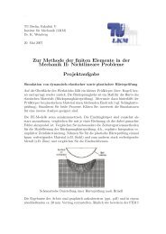
Real compression test results for cylinder lignite 

specimens are shown in Fig. 24a). Appearance of 

main diagonal crack that destroys the specimen 

can be seen. Before the main crack propagates a 

small piece of lignite at the lower left part is slivered 

from the specimen. This shown in Fig. 24b). 

The results of simulation show that lignite exhibits 

di€erent types of fracture behavior that 

ranges from brittle to quasi-plastic. These results 

agree with experimental data. It shows that the 

MCA method can be applied to stimulate fracture 

behavior of heterogeneous media under standard 

test conditions and complex loading that is di - 

cult to reproduce by experiments.


Fig. 23. Evolution of system of inter-automata bonds under loading for lignite specimens: a) Category II, b) Category IV, 

c) Category VI.


Fig. 24. Main stages of fracture of a) real lignite specimens under uniaxial compression, b) specimens fracture. 

6. Fracture energy under dynamic loading 

6.1. General remarks 

Structural dynamics involves cars or transport 

vehicles under impact. The analysis entails the 

transformation of kinetic energy of interaction to 

the energy required to fracture at least a portion of 

the structure. Similar problems also exist in materials 

science where modern materials are heterogeneous 

and have a complex internal structure. 

To optimize a material structure for carrying dynamic 

load it is necessary to account for redistribution 

of elastic energy connected with phase 

transition, generation and accumulation of microdamages, 

etc for they in¯uence the strength 

characteristics of the material [19,42±44]. These 

problems may be solved by the MCA method 

which has been successfully used for modeling 

fracture of the di€erent materials [14,16,44±46]. 

Several problems of practical interest will be 

presented. In particular, the frame in Fig. 25a) 

Fig. 25. Schematic of loading and fracture patterns: a) fracture patterns of the modeled structures t ˆ 355 ls, b) frame without 

inclusion base), c) frame with inclusions.

will be analyzed. The objective is to alter the local 

damping by changing the sti€ness such that energy 

would be more uniformly distributed. This would 

increase the load carrying capacity of the frame. 

The load is applied a ``piston'' with velocity of 5 

m/s, mechanical properties of the material correspond 

to those for ZrO2 ceramics. They have been 

obtained by the MCA method [14,16]. The sample 

width is 4 cm, the height is 5 cm and the size of the 

automaton is 0.1 cm. The parameters of the automata 

correspond to those for concrete. 

6.2. Fracture of structures 

Numerical experiments of ``collision'' show that 

the center and the corners behind the front wall of 

the modeled structure undergo maximal local deformation. 

Fig. 25b) shows the damage pattern. 

Hence, additional damping was added to these 

regions. This is accomplished by a reduction of the 

Young modulus by a factor of 2 when compared 

with the base structure material. The load carrying 

capacity of the structure is thus improved, and the 

damage is considerably less. Fig. 25c) also shows 

a linkage structure with additional damping at the 

same time t ˆ 355 ls as in Fig. 25b). By softening 

the local regions of the structure larger local displacements 

would result. This would reduce the 

stress concentration e€ects by a more uniform 

distribution of elastic energy. This would e€ectively 

raise the threshold of the energy absorbed by 

the structure before losing its carrying capacity. 

7. Conclusion 


This work has provided a description of the 

method of MCA and results for a limited number 

of applications. The method will be further expanded 

to cover a wide range of problems [47,48]. 

In particular it can treat problems at the mesolevel 

with explicit account of the anisotropy of representative 

volumes and at the macrolevel where 

approximate isotropy of the automata response 

could be assumed depending on the response 

function of a cellular automaton. One of the advantages 

of this approach is the direct simulation 

of the fracture process. Additional features of the 

MCA method can be developed. Change of the 

shape of automata is being considered. This would 

provide a wider range of plastic deformation simulation. 

3D MCA is being developed in addition to 

¯uids, chemical reactions, etc. 

References 

[1] P.A. Cundall, O.D.L. Strack, A discrete numerical model 

for granular assemblies, Geotechnique 29 1) 1979) 47. 

[2] P.A. Cundall, A computer simulations of dense sphere 

assembles, in: M. Satake, J.T. Jenkins Eds.), Micromechanics 

of Granular Materials, Elsevier, Amsterdam, 1988, 

p. 113. 

[3] H.J. Herrmann, Simulating granular media on the computer, 

in: P.L. Garrido, J. Marro Eds.), 3rd Granada 

Lectures in Computational Physics, Springer, Heidelberg, 

1995, p. 67. 

[4] J. Hemmingsson, H.J. Hermann, S. Roux, On stress 

networks in granular media, J. Phys. I 7 1997) 291. 

[5] O.R. Walten, Numerical simulation of inclined chute ¯ows 

of monodisperse, inelastic, frictional spheres, Mech. Mater. 

16 1993) 239. 

[6] O.R. Walten, Numerical simulation of inelastic, frictional 

particle-particle integration, in: M.C. Roco Ed.), Particulate 

Two-phase Flow, Butterworth±Heinemann, Boston, 

1993, p. 884. 

[7] S. Luding, Granular materials under vibration: Simulations 

of rotating spheres, Phys. Rev. E 52 4) 1995) 4442. 

[8] T. Poschel, Granular material ¯owing down an inclined 

chute: A molecular dynamic simulation, J. Phys. II 3 1993) 

27. 

[9] D. Greenspan, Particle modeling in science and technology, 

Coll. Math. Societatis Janos Bolyai 50 1988) 51. 

[10] G.P. Ostermeyer, Many particle systems, in: German- 

Polish Workshop 1995, Polska Akad. Nauk, WarszawaIns. 

Podst. Prob. Techniki 1996). 

[11] G.P. Ostermeyer, Mesoscopic particle method for description 

of thermomechanical and friction processes, Phys. 

Mesomech. 2 6) 1999) 23. 

[12] R.W. Hockney, J.W. Eastwood, Computer Simulation 

Using Particles, McGraw-Hill, New York, 1981. 

[13] D. Potter, Computational Physics, Wiley, London, 1973. 

[14] S.G. Psakhie, S.Yu. Korostelev, A.Yu. Smolin, A.I. 

Dmitriev, E.V. Shilko, D.D. Moiseyenko, E.M. Tatarintsev, 

S.V. Alexeev, Movable cellular automata method as a 

tool for physical mesomechanics of materials, Phys. 

Mesomech. 1 1) 1998) 89. 

[15] A.I. Dmitriev, S.Yu. Korostelev, G.P. Ostermeyer, S.G. 

Psakhie, A.Yu. Smolin, E.V. Shilko, Movable cellular 

automata method as a tool for simulation at the mesolevel, 

Proc. RAS Mech. Solids 6 1999) 87. 

[16] S.G. Psakhie, Y. Horie, S.Yu. Korostelev, A.Yu. Smolin, 

A.I. Dmitriev, E.V. Shilko, Movable cellular automata


method as a tool for simulation within the framework of 

physical mesomechanics of materials, Rus. Phys. J. 11) 

1995) 1157. 

[17] Yu.M. Svirezhev, Nonlinear Waves, Dissipative Structures, 

and Ecological Catastrophes, Nauka, Moscow, 1987. 

[18] S.M. Foiles, M.I. Baskes, M.S. Daw, Embeded-atommethod 

functions for the f.c.c. metals Cu, Ag, Au, Ni, Pd, 

Pt and their alloys, Phys. Rev. B 33 12) 1986) 7983. 

[19] V.E. Panin, Foundations of physical mesomechanics, Phys. 

Mesomech. 1 1) 1998) 5. 

[20] V.E. Panin Ed.), Physical Mesomechanics of Heterogeneous 

Media and Computer-aided Design of Materials, 

Cambridge Interscience Publishing, Cambridge, 1998. 

[21] S.G. Psakhie, D.D. Moiseyenko, A.Yu. Smolin, E.V. 

Shilko, A.I. Dmitriev, S.Yu. Korostelev, E.M. Tatarintsev, 

The features of fracture of heterogeneous materials and 

frame structures. Potentialities of MCA design, Comput. 

Mater. Sci. 16 1999) 333. 

[22] I.V. Kragelskii, Friction and Wear, Mashgiz, Moscow, 

1962. 

[23] W.W. Tworzydlo, W. Cecot, J.T. Oden, C.H. Yew, 

Computational micro- and macroscopic models of contact 

and friction: formulation, approach, and applications, 

Wear 220 1999) 113. 

[24] M.G. Rozman, M. Urbakh, J. Klafter, Stick-slip dynamics 

of interfacial friction, Physica A 249 1998) 184. 

[25] F. Raharijaona, X. Roizard, J. Stebut, Usuage of D 

roughness parameters adapted to the experimental simulation 

of sheet-tool contact during a drawing operation, 

Tribol. Int. 32 1999) 59. 

[26] A.F. Pimenov Ed.), Plastic Deformation of Construction 

Materials, Nauka, Moskow, 1988 in Russian). 

[27] J.F. Bell, Encyclopedia of Physics. Vol. VIa/1. Mechanics 

of Solids I, Springer, Berlin, 1973. 

[28] V.I. Syryamkin, V.Ye. Panin, Ye.Ye. Dyeryugin, A.V. 

Parfenev, G.V. Nerush, S.V. Panin, in: Physical Mesomechanics 

and Computer-aided Design of Materials, vol. 1, 

Nauka, Novosibirsk, 1995, p. 176 in Russian). 

[29] V.Ye. Panin, Methodology of Physical Mesomechanics as 

the basis for model construction of computer-aided design 

of materials, Rus. Phys. J. 11) 1995) 5. 

[30] S. Walfram, Theory and Application of Cellular Automata, 

World Scienti®c, Singapore, 1986. 

[31] G. Philippou, H. Kim, R. Rajagopalan, Comput. Mater. 

Sci. 4 2) 1995) 181. 

[32] V.Ye. Panin, V.A. Klimyonov, S.G. Psakhie, O.A. Atamanov, 

V.P. Bezborodov, V.V. Guzeev, S.P. E®menko, A.A. 

Zabolotskii, E.E. Kovalevskii, S.Yu. Korostelev, Advanced 

Materials and Technologies. Design of Advanced 

Materials and Hardening Processes, Nauka, Novosibirsk, 

1993 in Russian). 

[33] S.G. Psakhie, S.I. Negreskul, K.P. Zolnikov, S.Yu. Korostelev, 

A.V. Astapenko, E.V. Shil'ko, A.I. Dmitriev, S.V. 

Alekseev, D.Yu. Saraev, A.E. Kushnirenko, in: Physical 

Mesomechanics of Heterogeneous Media and Computer- 

aided Design of Materials, Cambridge Interscience Publishing, 

Cambridge, 1998. 

[34] S.G. Psakhie, A.Yu. Smolin, S.Yu. Korostelev, A.I. 

Dmitriev, E.V. Shil'ko, S.V. Alekseev, Pis'ma Zh. Tech. 

Phys. 21 20) 1995) 72 in Russian). 

[35] S.G. Psakhie, Ye.V. Shil'ko, A.I. Dmitriev, S.Yu. Korostelev, 

A.Yu. Smolin, Pis'ma Zh. Tech. Phys. 22 2) 1996) 90 

in Russian). 

[36] S.G. Psakhie, Y. Horie, S.Yu. Korostelev, A.Yu. Smolin, 

A.I. Dmitriev, E.V. Shil'ko, S.V. Alekseev, Movable 

cellular automata method as a new technique to simulate 

powder metallurgy materials, in: Proceedings of the International 

Conference on Deformation and Fracture in 

Structural PM Materials, Stara Lesna, Slovakia, 1996, pp. 

210±220. 

[37] I.S. Grigoriev, Ye.Z. Meilikhov Eds.), Physical Values. 

Handbook, Entergoatomizdat, Moscow, 1991 in Russian). 

[38] A.M. Neville, Properties of Concrete, Wiley, New York, 

1973. 

[39] S. Zavshek, Dangerous occurences in the Velenje pit, in: 

Materials of 22nd Meeting of Miners, Izlake, Slovenia, 

1997. 

[40] M. Markich, R.F. Sachsenhofer, Petrogra®c composition 

and decompositional environments of the pliocene Velenje 

lignite seam, Int. J. Coal Geol. 11) 1997) 229±254. 

[41] M. Markich, S. Zavshek, Lithotype characterization of the 

Velenje lignite. A short working issue, Velenje, Slovenia, 

1999. 

[42] E. Haug, J. Clinckemaillie, X. Ni, A.K. Pickett, T. 

Queckbarner, Recent trends and advances in crash simulation 

and design of vehicles, in: International Crashworthiness 

and Design Symposium ICD '95, University of 

Valenciennes, May 3±4, 1995. 

[43] G. Lonsdale, J. Clinckemaillie, S. Vlachoutsis, J. Dubois, 

Communication requirements in parallel crashworthiness 

simulation, in: Lecture Notes in Computer Science, vol. 

796, Springer, Berlin, 1994. 

[44] S.G. Psakh'e, D.D. Moiseenko, A.I. Dmitriev, E.V. 

Shil'ko, S.Yu. Korostelev, A.Yu. Smolin, E.E. Deryugin, 

S.N. Kul'lkov, A possible method of computer-aided 

design of materials with a highly porous matrix, Tech. 

Phys. Lett. 24 2) 1998) 154±156. 

[45] S.G. Psakhie, E.V. Shilko, A.I. Dmitriev, S.Yu. Korostelev, 

A.Yu. Smolin, E.N. Korostelev, Self-organization 

e€ect in process of deformation of PM materials, Tech. 

Phys. Lett. 22 12) 1996) 69±74. 

[46] S.G. Psakhie, A.Yu. Smolin, E.V. Shilko, S.Yu. Korostelev, 

A.I. Dmitriev, S.V. Alekseev, About the features of 

transient to steady state deformation of solids, J. Mater. 

Sci. Technol. 13 11) 1997) 69±72. 

[47] S. Wolfram, Statistical mechanics of cellular automata, 

Rev. Mod. Phys. 55 1983) 601±620. 

[48] A.Yu. Loskutov, A.S. Mikhailov, Introduction to Synergetic, 

Nauka, Moscow, 1990.

Movable cellular automata method for simulating materials with ...

Create successful ePaper yourself

Delete template?

Save as template?