Chapter 3: Dynamic programming - mechatronics

Chapter 3 

Dynamic programming 

3.1 Introduction 

A very powerful method for optimization of a system that can be separated into 

stages is dynamic programming developed by Bellman [2]. The main concept of this 

technique lies in the principle of optimality which can be stated as follows: 

An optimal policy has the property that whatever the initial state and the initial 

decision are, the remaining decisions must constitute an optimal policy with regard to 

the state resulting from the first decision. 

Many engineering systems are in the form of individual stages, or can be broken 

into stages, so the idea of breaking up a complex problem into simpler subproblems, so 

that optimization could be carried out systematically by optimizing the subproblems, 

was received enthusiastically. Numerous applications of the principle of optimality 

in dynamic programming were given by Bellman and Dreyfus [3], and there was a 

great deal of interest in applying dynamic programming to optimal control problems. 

In the 1960’s many books and numerous papers were written to explore the use 

of dynamic programming as a means of optimization for optimal control problems. 

A very readable book was written by Aris [1]. Since an optimal control problem, 

involving optimization over a trajectory, can be broken into a sequence of time stages, 

it appeared that dynamic programming would be ideally suited for such problems. 

To understand the principle of optimality and to see the beauty of dynamic programming 

we wish topresent a few examples. 

3.2 Examples 

In order to understand and appreciate dynamic programming, we present several 

examples. 

c○ 2000 by Chapman & Hall/CRC

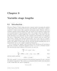
3.2.1 A simple optimal path problem 

Let us consider asituation depicted in Figure 3.1, where there are different paths that 

could be taken in going from A to B. The costs for sections of the paths are shown 

by the numbers. Suppose we wish tofind the path, always moving tothe right, such 

that the total cost in going from A to B is minimized. For ease of discussion, the 

nodes are labelled by the letters a, b, ···,l. 

Figure 3.1: Optimal path problem 

Starting at node a, we find that there is only one way togotoB and the associated 

cost is 5, so we associate the minimum cost 5 with node a. Similarly, there is only 

one way to proceed from node b and the cost is 3 plus the cost from going from node 

a to B. Thus we associate the minimum cost 8 with the node b. Proceeding to node 

c, since we are always going from left to right, we see that there is only one way to 

get to B and the associated cost is 7. At the node d, there are two options: one is 

toproceed tonode c and the other is toproceed tonode a. It is noted that here it 

does not make any difference, since the cost with each alternative is 11. Therefore we 

assign the minimum cost 11 to node d. 

At node e there are alsotwoways of proceeding. We can gotoeither node d orto 

node b. In the former, the cost is 5 + 11 = 16, and for the latter the cost is 5 + 8 =13. 

We compare these two numbers and choose the path that gives the smaller number, 

namely the path e to b, and associate with node e the minimum cost 13. Similarly 

at node f we compare the two costs 9 + 13 = 22 and 4 + 8 = 12, and associate the 

minimum cost 12 with the node f and the path f to b rather than f to e. At no de 

g there is only one way of proceeding, so the minimum cost associated with node g 


is 8 + 7 = 15. At node h we compare the two costs 1+15=16and3+11=14, 

and choose the path h to d. Atnodei comparison of two costs gives us the minimum 

cost of 17 along the path i to h. Atnodej the minimum cost 14 is achieved by going 

from j to f. At the node k we compare the two costs 4+15=19and9+14=23, 

and choose the path k to g. At the node l we compare the two costs 5+19=24and 

2 + 17 = 19 and choose the path l to i which gives the minimum cost of 19. 

Now we proceed tothe starting point A. Here we have twoways of proceeding. 

For the path A to l the cost is 3 + 19 = 22, and for the path A to j the cost is 9 + 

14 = 23. Therefore we conclude that the minimum cost in going from A to B is 22 

and that there are twopaths that yield this cost: AlihdcB and AlihdaB. 

We note here that instead of doing the minimization as a whole problem, we solve 

a sequence of very simple minimization problems which involve comparing two numbers 

at the nodes. Some of the nodes were actually “free” where no optimization was 

necessary. Also it is observed that it is not possible to miss the global minimum, and 

if there is more than one path that yields the minimum, the method captures all of 

them, as was illustrated here. The computational advantage of this approach over 

exhaustive enumeration becomes more apparent as the size of the problem increases. 

For example, if instead of the 3 × 3 grid, we would have a 10 × 10 grid, the approach 

with dynamic programming could still be easily done by hand, but exhaustive 

enumeration of all the possible paths would be unrealistic. 

We now turn to a very similar type of a problem involving the scheduling of jobs 

that are to be done on a single facility in such a way that the cost would be minimized 

[4]. 

3.2.2 Job allocation problem 

Let us consider a set of P jobs, called J1,J2, ···,JP tobe executed on a single facility. 

Associated with each job Jn is a time of execution τn and a cost function cn(t) giving 

the cost associated with completing the job at time t. For simplicity, we assume that 

only one job is executed at a time, that there is no interruption in a job once it is 

started, and the facility is constantly in use. The problem is to choose the ordering of 

the jobs such that the total cost is minimized. The performance index is thus chosen 

tobe 

P 

I = ck(tk), (3.1) 

k=1 

and we wish todetermine the order in which the jobs are tobe executed sothat the 

performance index is minimized. For all possible orderings we need to examine P ! 

schedules, which becomes unmanageable when P is large. For this type of problem 

dynamic programming is well suited. We illustrate this with the case where P =5 

jobs. This problem is very similar to the optimal path problem discussed earlier. We 

picture the problem as involving 5 stages. At stage 1 we have 5 jobs and at stage 

5 we have a single job to consider. We start at the last stage (stage 5) involving a 


single job. There is no optimization possible at this stage. The cost of doing job i 

incurs a cost ci(τi). 

Now let us consider stage 4 where two jobs are to be considered. There are 10 

possible sets of two jobs to consider. Each set has two permutations. For example, 

if we consider jobs J1 and J2, we ask whether the arrangement should be J1 followed 

by J2 denoted by J1J2, or whether it should be J2J1. For the order J1J2 the cost is 

c1(τ1) +c2(τ2 + τ1) and for the order J2J1 the cost is c2(τ2) +c1(τ1 + τ2). These costs 

are different since the cost of a particular job is dependent on the time when that job 

is finished. The two numbers are compared, and suppose that it is found that the 

latter arrangement gives a smaller cost. Then we know that in doing jobs J1 and J2, 

job J2 should be done first followed by J1. We carry out this comparison with the 

other 9 sets and then construct a table showing the arrangement of two jobs to yield 

the minimum cost, as is shown in Table 3.1. 

Table 3.1: Order and minimum cost for 2 jobs 

Ordered Jobs Minimum cost 

J2J1 c2(τ2)+c1(τ2 + τ1) 

J3J1 c3(τ3)+c1(τ3 + τ1) 

J1J4 c1(τ1)+c4(τ4 + τ1) 

J1J5 c1(τ1)+c5(τ5 + τ1) 

J2J3 c2(τ2)+c3(τ2 + τ3) 

J4J2 c4(τ4)+c2(τ4 + τ2) 

J2J5 c2(τ2)+c5(τ2 + τ5) 

J4J3 c4(τ4)+c3(τ4 + τ3) 

J3J5 c3(τ3)+c5(τ3 + τ5) 

c5(τ5)+c4(τ5 + τ4) 

J5J4 

Now we proceed to stage 3 where three jobs are to be considered. There are 10 

possible sets of 3 jobs taken from 5 jobs. Let us choose the set consisting of jobs J1, 

J2 and J3. Weuse the information in Table 3.1 to reduce the number of calculations 

required todetermine the order. If J1 is last, then we know the order in which jobs 

J2 and J3 are to be done and the cost associated with these two jobs from the fifth 

line of Table 3.1. All that is necessary is to add the additional cost c1(τ2 + τ3 + τ1). 

Similarly, if J2 is done last, the cost is the corresponding entry for jobs 1 and 3 from 

the second line of Table 3.1 plus c2(τ1 + τ3 + τ2); and if J3 is done last, the cost is the 

correspondingentryforjobs1and2fromthefirstlineofTable3.1plusc3(τ1+τ2+τ3). 

These three costs are compared, and the arrangement that gives the minimum cost 

is kept. Let us suppose that of these 3 arrangements, the order J2J1J3 gives the least 

cost. This entry appears on the first line of Table 3.2. This procedure is repeated 


for the other 9 sets and the table is completed, showing the minimum costs for three 

jobs. 



J2J1J3 c2(τ2)+c1(τ2 + τ1)+c3(τ1 + τ2 + τ3) 

J3J1J4 c3(τ3)+c1(τ3 + τ1)+c4(τ1 + τ3 + τ4) 

J1J4J2 c1(τ1)+c4(τ4 + τ1)+c2(τ1 + τ4 + τ2) 

J1J5J3 c1(τ1)+c5(τ5 + τ1)+c3(τ1 + τ5 + τ3) 

J2J3J4 c2(τ2)+c3(τ2 + τ3)+c4(τ2 + τ3 + τ4) 

J4J2J5 c4(τ4)+c2(τ4 + τ2)+c5(τ4 + τ2 + τ5) 

J2J5J1 c2(τ2)+c5(τ2 + τ5)+c1(τ2 + τ5 + τ1) 

J4J3J5 c4(τ4)+c3(τ4 + τ3)+c5(τ4 + τ3 + τ5) 

J3J5J2 c3(τ3)+c5(τ3 + τ5)+c2(τ3 + τ5 + τ2) 

c5(τ5)+c4(τ5 + τ4)+c1(τ5 + τ4 + τ1) 

J5J4J1 

Now we proceed to stage 2 where 4 jobs are to be considered. There are 5 possible 

sets of 4 jobs that can be chosen from 5 jobs. Let us choose the set consisting of jobs 

J1, J2, J3, and J5. Weuse the information in Table 3.2 to determine the order and 

the minimum cost for the first three jobs, and we simply add the cost of doing the 

last job. If J1 is done last, then we know the order in which jobs J2, J3 and J5 are 

to be done and the cost associated with these three jobs from Table 3.2. All that is 

necessary is to add the additional cost c1(τ2 + τ3 + τ5 + τ1). We proceed for the other 

three cases, where J2, J3, orJ5 is done last as before and compare the 4 cost values 

togive the arrangement yielding the smallest cost. Repeating the procedure with the 

other 4sets provides the information that can be displayed in Table 3.3. 



J1J4J2J3 c1(τ1)+c4(τ4 + τ1)+c2(τ1 + τ4 + τ2)+c3(τ1 + τ4 + τ2 + τ3) 




c3(τ3)+c5(τ3 + τ5)+c2(τ3 + τ5 + τ2)+c1(τ3 + τ5 + τ2 + τ1) 

J3J5J2J1 


Let us now proceed to stage 1 where 5 jobs are to be considered. There is only one 

set to consider. We ask ourselves which job is to be done last. If J4 is done last, then 

the minimum cost of doing the other 4jobs is obtained from the last line of Table 3.3 

and we simply add the cost of doing J4, namely, c4(τ1 + τ2 + τ3 + τ4 + τ5). Similarly, 

we find from the second line of Table 3.3 the order and the minimum cost of doing 

the first four jobs if J2 is done last and simply add the cost c2(τ1 + τ2 + τ3 + τ4 + τ5). 

We continue the process for when J3 is done last, when J4 is done last, and when J1 

is done last. These 5 values of cost are compared and the minimum of these gives us 

the order of the 5 jobs such that the cost is minimized. 

We see in this example that the calculations proceed in a systematic way, so that 

at each stage the optimization involves only the addition of a single job to those 

that have been already optimally calculated. The procedure is ideally suited for the 

use of a digital computer where the same calculational procedure is used repeatedly 

numerous times. Instead of simply providing a numerical approach to optimization 

problems, dynamic programming also provides functional relationships as can be seen 

in the next example. 

3.2.3 The stone problem 

Let us illustrate the use of dynamic programming in solving the problem of how high 

a stone rises when tossed upwards with a velocity of v0. Let us assume that air 

resistance cannot be ignored, so the equation of motion for the stone can be written 

as 

dv 

= −g − kv2 

(3.2) 

dt 

with the initial condition v = v0 at t = 0. It is clear that the height is a function 

of the initial velocity. Let us break the trajectory into two parts: the first part is 

the short distance the stone travels in a short time ∆t and the second part is the 

remainder of the trajectory 

h(v0) =v0∆t + h(v0 + dv 

dt ∆t)+O(∆t2 ). (3.3) 

Now let us expand the second term on the right hand side by Taylor series, retaining 

only the first twoterms, and using Eq.(3.2) togive 

h(v0) =v0∆t + h(v0) − [(g + kv 2 0)∆t] dh(v0) 

+ O(∆t 

dv0 

2 ). (3.4) 

When we rearrange Eq. (3.4) and divide by ∆t, we get 

c○ 2000 by Chapman & Hall/CRC 

dh(v0) 

dv0 

= 

v0 

g + kv2 0 

+ O(∆t). (3.5)

Now we let ∆t → 0 to yield a first order ordinary differential equation 

dh(v0) 

= 

dv0 

v0 

g + kv2 , 

0 

(3.6) 

which can be immediately integrated with the given initial condition to give 

h(v0) = 1 

2k ln(1 + kv2 0 

). 

g 

(3.7) 

When k is negligibly small then we see that h(v0) → v2 0/2g, a result which can be 

obtained by equating the kinetic energy at the initial time and the potential energy 

at the maximum height. 

3.2.4 Simple optimal control problem 

Let us consider a rather simple optimal control problem where a linear discrete scalar 

system is given in the form 

x(k +1)=ax(k)+bu(k), k =0, 1, 2, ···,P − 1, (3.8) 

where the initial state x(0) is given, and the final state x(P ) = 0. We assume there 

are no constraints placed on the control u(k). The optimal control problem is to 

choose u(k),k =0, 1, 2, ···,P − 1 sothat the performance index 

P 

I[x(0),P]= [x 

k=1 

2 (k)+u 2 (k − 1)] (3.9) 

is minimized. Here we have shown the explicit dependence of the performance index 

on the initial state and the number of steps P . Naturally the performance index is 

also a function of the control policy which has to be chosen for minimization. To solve 

this problem by dynamic programming we first consider a single stage problem and 

then progressively increase the number of stages until the posed problem is solved. 

P=1 

When we have a single stage problem, the performance index is 

I[x(0), 1] = x 2 (1) + u 2 (0) (3.10) 

and no minimization is possible, since the specification of the final condition requires 

that we use 

x(1) − ax(0) 

u(0) = = − 

b 

a 

x(0). (3.11) 

b 

The value of the performance index is 


I[x(0), 1] = a2 

b 2 x2 (0). (3.12)

Next we consider P = 2 stages. 

P=2 

With twostages we start at x(0) proceed to x(1) and then gotox(2) = 0. The 

performance index to be minimized is 

I[x(0), 2] = x 2 (1) + u 2 (0) + x 2 (2) + u 2 (1) = x 2 (1) + u 2 (0) + u 2 (1). (3.13) 

Once we get to x(1), we already know how to get to x(2) = 0, because that is a 

1-stage problem that was solved above. We therefore have 

u(1) = − a 

x(1). (3.14) 

b 

The performance index becomes 

I[x(0), 2]=(1+ a2 

b 2 )x2 (1) + u 2 (0). (3.15) 

By using Eq. (3.8) with k = 0, we can rewrite the performance index as an explicit 

function of u(0) only, namely, 

I[x(0), 2]=(1+ a2 

b 2 )[ax(0) + bu(0)]2 + u 2 (0). (3.16) 

Differentiating Eq. (3.16) with respect tou(0) gives 

dI[x(0), 2] 

du(0) 

a2 

=2b(1 + )[ax(0) + bu(0)] + 2u(0). (3.17) 

b2 Since the second derivative of the performance index is positive, the choice of u(0) to 

minimize the performance index is obtained from the stationary condition that yields 

We are now ready to consider P = 3 stages. 

u(0) = −( ab +(a3 /b) 

1+a2 )x(0). (3.18) 

+ b2 P=3 

The pattern for calculations becomes clear with the addition of one more stage. 

With P = 3, the performance index is 

I[x(0), 3] = x 2 (1) + u 2 (0) + x 2 (2) + u 2 (1) + u 2 (2), (3.19) 

since x(3) = 0. Here we know that the optimal choices for u(2) and u(1), as determined 

before, are 

u(2) = − a 

x(2) 

b 

(3.20) 


and 

u(1) = −( ab +(a3 /b) 

1+a2 )x(1). (3.21) 

+ b2 The performance index can now be expressed as an explicit function of u(0), and the 

process can be repeated. 

Although analytically this process is tedious after a while, numerically such optimization 

can be done very easily. By using dynamic programming, the solution of P 

simultaneous equations is replaced by a procedure which handles one single equation, 

but does it P times. Thus parallel computation is replaced by serial computation. 

3.2.5 Linear optimalcontrolproblem 

As a further example we consider a linear optimal control problem where the system 

is described by 

x(k +1)=Φx(k)+Ψu(k), k =0, 1, ···,P − 1, (3.22) 

where Φ and Ψ are constant matrices, and the initial condition x(0) is given. The 

performance index is assumed to have the quadratic form 

P 

I[x(0),P]= [x 

k=1 

T (k)Qx(k)+u T (k − 1)Ru(k − 1)] (3.23) 

where R is a positive definite symmetric matrix and Q is a positive semi-definite 

symmetric matrix. Let us define 

I 0 [x(0),P] = minI[x(0),P] (3.24) 

such that I 0 [x(0),P] is the optimal value of the performance index over P stages of 

control. Thus 

I 0 [x(0),P] = min 

u(0) min 

u(1) 

P 

[x 

u(P −1) 

k=1 

T (k)Qx(k)+u T (k − 1)Ru(k − 1)]. (3.25) 

··· min 

We can use the principle of optimality in dynamic programming to rewrite the expression 

as 

I 0 [x(0),P] = min 

u(0) [xT (1)Qx(1) + u T (0)Ru(0) + I 0 [x(1),P − 1]], (3.26) 

which provides a recurrence relationship of dynamic programming. 

Let us assume that the optimum performance index can be written as 


I 0 [x(0),P]=x(0) T JP x(0) (3.27)

where JP is a positive semi-definite symmetric matrix. Then 

and Eq. (3.26) becomes 

I 0 [x(1),P − 1] = x(1) T JP −1x(1) (3.28) 

I 0 [x(0),P] = min 

u(0) [xT (1)(Q + JP −1)x(1) + u T (0)Ru(0)], (3.29) 

where x(1) is obtained from Eq. (3.22) as an explicit function of x(0) and u(0). As 

is shown in [4], after some mathematical manipulations we get the optimal control 

policy 

u 0 (k) =−KP −kx(k), (3.30) 

where the feedback gain matrix KP −k is obtained by solving recursively 

and 

KP −k =[Ψ T (Q + JP −k−1)Ψ + R] −1 Ψ T (Q+J P −k−1)Φ (3.31) 

JP −k = Φ T (Q+J P −k−1)(Φ − ΨKP −k) (3.32) 

with the initial condition J0 = 0. Therefore, dynamic programming can be used 

for optimal control of high dimensional systems if the state equation is linear, the 

performance index is quadratic, and the control is unbounded. For general nonlinear 

optimal control problems, where the solution can be obtained only numerically, there 

are some inherent difficulties in the use of dynamic programming, as will be pointed 

out in Section 3.3. 

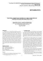
3.2.6 Cross-current extraction system 

Let us consider the liquid-liquid cross-current extraction system with immiscible solvents 

of a single solute, as used by Lapidus and Luus [4] to illustrate optimization 

techniques. The system consists of three stages, as is shown in Figure 3.2. The 

solvent flow rate in the raffinate stream is denoted by q, and the solvent flow rate 

in the extract streams entering and leaving stage k is denoted by w(k). The solute 

concentration leaving stage k in raffinate is x(k), and the solute concentration leaving 

stage k in extract is y(k). 

Mass balance around stage k yields 

x(k) =x(k − 1) − u(k)y(k), k =1, 2, 3, (3.33) 

where u(k) = w(k)/q. We assume equilibrium between the raffinate and extract 

phases at each stage, and that the solute concentrations in the two phases can be 

expressed through the linear relationship 


y(k) =αx(k). (3.34)

Figure 3.2: Cross-current extraction system 

The state equation can then be written as 

x(k +1)= 

x(k) 

, k =0, 1, 2. (3.35) 

1+αu(k +1) 

We would like to choose the flow rates w(1),w(2), and w(3), or in normalized 

form u(1),u(2), and u(3), so that we remove the maximum amount of solute from 

the raffinate stream. However, there is a cost associated with the use of the extract 

solvent. Therefore, the performance index to be maximized is chosen as 

I[x(0), 3]=[x(0) − x(3)] − θ[u(1) + u(2) + u(3)], (3.36) 

where θ is a cost factor associated with the use of extract solvent. This optimization 

problem is well suited for dynamic programming. When there are P stages, then the 

performance index becomes 

P 

I[x(0),P]=[x(0) − x(P )] − θ u(i). (3.37) 

i=1 

As we did with the simple optimal control problem earlier, we solve this optimization 

problem by first considering P = 1 and then increasing P until we reach P =3. 

P=1 

When we have a single stage, the performance index is 

where 


I[x(0), 1]=[x(0) − x(1)] − θu(1) (3.38) 

x(1) = 

x(0) 

. (3.39) 

1+αu(1)

The maximum value of the performance index is thus 

I 0 αx(0) 

[x(0), 1] = max[u(1)( 

− θ)]. (3.40) 

u(1) 1+αu(1) 

By taking the derivative of the expression with respect to u(1) and setting it tozero, 

we get 

αx(0) − θ(1 + αu(1)) 2 

(1 + αu(1)) 2 =0, (3.41) 

so that the optimal value for u(1) is 

u 0 (1)=[ x(0) 1 

] 2 − 

αθ 1 

. (3.42) 

α 

From Eq. (3.39) it follows that 

x(1)=[ θx(0) 1 

] 2 (3.43) 

α 

and the maximum performance index with the single stage is 

I 0 [x(0), 1] = x(0) − 2[ θx(0) 1 

] 2 + 

α θ 

. (3.44) 

α 

P=2 

From the principle of optimality in dynamic programming, we can write the maximum 

value of the performance index as 

I 0 αx(0) 

[x(0), 2] = max[u(1)( 

u(1) 1+αu(1) − θ)+I0 [x(1), 1]]. (3.45) 

However, we have already calculated the optimum value of the performance index for 

the single stage. All we have todois tochange x(0) to x(1) in Eq. (3.44). Thus 

Therefore, 

I 0 [x(1), 1] = x(1) − 2[ θx(1) 1 

] 2 + 

α θ 

. (3.46) 

α 

I 0 αx(0) 

x(0) 

[x(0), 2] = max[u(1)( 

− θ)+ 

u(1) 1+αu(1) 1+αu(1) 

θx(0) 1 

− 2[ 

] 2 + 

α(1 + αu(1)) θ 

]. (3.47) 

α 

Differentiating the expression with respect to u(1) and putting the result equal to 

zerogives 

−θ(1 + αu(1)) 2 + θx(0)[ 


α(1 + αu(1)) 

] 

θx(0) 

1 

2 =0, (3.48)

so that the optimal value for u(1) is 

and 

u 0 (1)=[ x(0) 

α2 1 

] 3 − 

θ 1 

α 

(3.49) 

x(1)=[ x2 (0)θ 1 

] 3 . (3.50) 

α 

The optimal performance index with P =2is 

I 0 [x(0), 2] = x(0) − 3[ θ2x(0) α2 ] 1 

3 + 2θ 

. (3.51) 

α 

At this time it is interesting tonote that 

u 0 (2)=[ x(1) 1 

] 2 − 

αθ 1 

α =[[x2 (0)θ 

α 

1 1 1 

] 3 ] 2 − 

αθ 1 

α = u0 (1). (3.52) 

Therefore, the optimal policy is to distribute the extract solvent in equal quantities 

in each stage. 

P=3 


I 0 αx(0) 

[x(0), 3] = max[u(1)( 

u(1) 1+αu(1) − θ)+I0 [x(1), 2]], (3.53) 

where the last term that has been previously calculated is 

I 0 [x(1), 2] = x(1) − 3[ θ2x(1) α2 ] 1 

3 + 2θ 

. (3.54) 

α 

After substituting Eq. (3.54) intoEq. (3.53) and differentiating the expression with 

respect to u(1), we get for the stationary condition 

sothat 

θ(1 + αu(1)) 2 = θ2x(0) α [ 

θ2x(0) α2 (1 + αu(1)) 

]− 2 

3 , (3.55) 

1+αu(1)=[ x(0)α 

] 

θ 

1 

4 . (3.56) 

Therefore, the optimal value for control to the first stage is 


u 0 (1)=[ x(0) 

α3 1 

] 4 − 

θ 1 

, (3.57) 

α

and the solute concentration in the raffinate stream leaving this stage is 


x(1)=[ x3 (0)θ 1 

] 4 . (3.58) 

α 

I 0 [x(0), 3] = x(0) − 4[ θ3x(0) α3 ] 1 

4 + 3θ 

. (3.59) 

α 

It is easy to show that the optimal control policy is 

u 0 (1) = u 0 (2) = u 0 (3), (3.60) 

showing that the extract solvent should be distributed in equal quantities in each 

stage. 

3.3 Limitations of dynamic programming 

Although dynamic programming has been successfully applied to some simple optimal 

control problems, one of the greatest problems in using dynamic programming 

for optimal control of nonlinear systems, however, is the interpolation problem encountered 

when the trajectory from a grid point does not reach exactly the grid point 

at the next stage [4]. This interpolation difficulty coupled with the dimensionality 

restriction and the requirement of a very large number of grid points limits the use of 

dynamic programming to only very simple optimal control problems. The limitations 

imposed by the “curse of dimensionality” and the “menace of the expanding grid” 

for solving optimal control problems kept dynamic programming from being used for 

practical types of optimal control problems. 

3.4 References 

[1] Aris, R.: Discrete dynamic programming, Blaisdell Publishing Co., New York, 

1964. 

[2] Bellman, R.E.: Dynamic programming, Princeton University Press, 1957. 

[3] Bellman, R. and Dreyfus, S.: Applied dynamic programming, Princeton 

University Press, 1962. 

[4] Lapidus, L. and Luus, R.: Optimal control of engineering processes, Blaisdell, 

Waltham, Mass., 1967.

Chapter 3: Dynamic programming - mechatronics

You also want an ePaper? Increase the reach of your titles

Delete template?

Save as template?