On Distributed Order Lead-Lag Compensator* - mechatronics - Utah ...
On Distributed Order Lead-Lag Compensator* - mechatronics - Utah ...
On Distributed Order Lead-Lag Compensator* - mechatronics - Utah ...

You also want an ePaper? Increase the reach of your titles
YUMPU automatically turns print PDFs into web optimized ePapers that Google loves.
Proceedings of FDA’10. The 4th IFAC Workshop Fractional Differentiation and its Applications.<br />
Badajoz, Spain, October 18-20, 2010 (Eds: I. Podlubny, B. M. Vinagre Jara, YQ. Chen,<br />
V. Feliu Batlle, I. Tejado Balsera). ISBN 9788055304878.<br />
<strong>On</strong> <strong>Distributed</strong> <strong>Order</strong> <strong>Lead</strong>-<strong>Lag</strong> Compensator ⋆<br />
Yan Li ∗,∗∗∗ Hu Sheng ∗∗,∗∗∗ YangQuan Chen ∗∗∗<br />
∗ School of Control Science and Engineering, Shandong University, Jinan,<br />
Shandong 250061, P. R. China. (e-mail: liyan cse@sdu.edu.cn)<br />
∗∗ Department of Electronic Engineering, Dalian University of Technology,<br />
Dalian 116024, P. R. China. (e-mail: shenghu 01@163.com)<br />
∗∗∗ Center for Self-Organizing and Intelligent Systems (CSOIS), Electrical<br />
and Computer Engineering Department, <strong>Utah</strong> State University, Logan, UT<br />
84322, USA. (e-mail: yangquan.chen@usu.edu)<br />
Abstract: In this paper, we derive the impulse response of the distributed order lead-lag compensator.<br />
Based on the derived analytical impulse response, we present how to compute the distributed order leadlag<br />
compensator in Matlab. The analytical method discussed in this paper is compared with the numerical<br />
inverse Laplace transform (NILT) method which shows two advantages of the analytical one. The illustrated<br />
figures in time domain are provided as proof of concept.<br />
Keywords: <strong>Distributed</strong> order, <strong>Lead</strong>-lag compensator, Controller design, Fractional Calculus.<br />
1. INTRODUCTION<br />
Fractional calculus is a mathematical discipline which deals with<br />
derivatives and integrals of arbitrary real or complex orders Oldham<br />
et al. (1974); Miller et al. (1993); Podlubny (1999); Kilbas<br />
et al. (2006). It was proposed more than 300 years ago and the<br />
theory was developed mainly in the 19th. Several books Oldham<br />
et al. (1974); Miller et al. (1993); Podlubny (1999); Kilbas et al.<br />
(2006) provide a good source of references on fractional calculus.<br />
It has been shown that there are a growing number of physical<br />
systems whose behavior can be compactly described using<br />
fractional-order system (or systems containing fractional derivatives<br />
and integrals) theory Hartley et al. (1999, 2003). Moreover,<br />
fractional calculus has also been applied to almost every direction<br />
of control theory and its applications Podlubny (1999); Kilbas<br />
et al. (2006); Oustaloup (1991); Podlubny (1999); Sabatier et al.<br />
(2007).<br />
The idea of distributed order equation was first proposed by<br />
M. Caputo in 1969 Caputo (1969) and partly solved by him<br />
in 1995 Caputo (1995). Those distributed order equations were<br />
introduced in the constitutive equations of dielectric media Caputo<br />
(1995) and in the diffusion equation Bagley et al. (2000).<br />
In Lorenzo et al. (2002), the authors studied the rheological<br />
properties of composite materials. The distributed order fractional<br />
kinetics was discussed in Sokolov et al. (2004). In Umarov<br />
et al. (2006), the multi-dimensional random walk models were<br />
governed by distributed fractional order differential equations.<br />
The ultraslow and lateral diffusion processes were discussed<br />
in Kochubei (2008). For the theories of distributed order equations,<br />
we cite Hartley et al. (1999, 2003); Caputo (1995); Bagley<br />
et al. (2000); Lorenzo et al. (2002); Sokolov et al. (2004);<br />
Umarov et al. (2006); Kochubei (2008); Lorenzo et al. (1998);<br />
Caputo (2001); Tsao (1987); Bohannan (2000); Connolly (2004);<br />
Atanackovic et al. (2005); Mainardi et al. (2007a,b); Srokowski<br />
(2008); Sun et al. (2009, 2010); Chen et al. (2009); Diethelm<br />
⋆ This work is partially supported by the Projects of National 863 Program(Grant<br />
No. 2009AA04Z220 and 2006AA040206) and the Shandong University Research<br />
Startup Fund to Yan Li.<br />
et al. (2009); Atanackovic et al. (2009a,b,c). It can be proved<br />
that both integer and fractional order systems are special cases<br />
of distributed order systems Lorenzo et al. (2002). Particularly<br />
when the complexity, networks, nonhomogeneous, multi-scale<br />
and multi-spectral are considered, the distributed order operator<br />
becomes a more precise tool to describe the above phenomena<br />
Hartley et al. (1999, 2003); Caputo (1995); Bagley et al.<br />
(2000); Lorenzo et al. (2002); Sokolov et al. (2004); Umarov et al.<br />
(2006); Kochubei (2008); Lorenzo et al. (1998); Caputo (2001);<br />
Tsao (1987); Bohannan (2000); Connolly (2004); Atanackovic<br />
et al. (2005); Mainardi et al. (2007a,b); Srokowski (2008); Sun<br />
et al. (2009, 2010); Chen et al. (2009); Diethelm et al. (2009);<br />
Atanackovic et al. (2009a,b,c); Adams et al. (2008); Atanackovic<br />
et al. (2007); Mainardi et al. (2007). Therefore, motivated by<br />
the previous references Goodwin et al. (2000); Nise (2004) and<br />
the applications of the fractional distributed operators to control,<br />
filtering and signal processing, a distributed order lead-lag<br />
compensator is derived step by step in the following. Firstly, the<br />
classical integer-order lead-lag compensator can be rewritten as:<br />
s + µ<br />
s + λ =<br />
∞<br />
−∞<br />
δ(α − 1)<br />
α s + µ<br />
dα,<br />
s + λ<br />
where λ = µ are arbitrary positive real constants, δ(·) denotes<br />
the Dirac-Delta function and<br />
s+µ<br />
s+λ<br />
α<br />
is a fractional-order lead-<br />
lag compensator with order α ∈ R. Moreover, the summation<br />
of a series of fractional order integrators/differentiators can be<br />
expressed as:<br />
<br />
k<br />
s + µ<br />
s + λ<br />
αk<br />
=<br />
∞<br />
−∞<br />
<br />
<br />
s α + µ<br />
δ(α − αk) dα,<br />
s + λ<br />
k<br />
where k can belong to any countable or non countable set. Now,<br />
<br />
it is straightforward to replace δ(α − αk) by a weighted<br />
kernel w(α). It follows that the right side of the above equation<br />
becomes<br />
∞ α s + µ<br />
w(α) dα,<br />
s + λ<br />
Page 1 of 5<br />
−∞<br />
k<br />
Article no. FDA10-137
where w(α) is independent of time and the above equation<br />
defines a distributed order lead-lag compensator. Particularly,<br />
when w(α) is a piecewise function,<br />
∞ α s + µ<br />
w(α) dα =<br />
s + λ<br />
<br />
−∞<br />
l<br />
bl<br />
w(αl)<br />
al<br />
α s + µ<br />
dα,<br />
s + λ<br />
where l belongs to a countable set, al, bl are real numbers, αl ∈<br />
(al, bl) and w(α) is a constant on α ∈ (al, bl). Based on the<br />
above discussions, without loss of generality, we focus on the<br />
discussions of the uniform distributed order lead-lag compensator<br />
where 0 < a < b ≤ 1.<br />
b<br />
a<br />
α s + µ<br />
dα,<br />
s + λ<br />
In this paper, we first focus on the inverse Laplace transform of<br />
the uniformly distributed order lead-lag compensator by cutting<br />
the complex plane and computing the complex integrals. The<br />
derived results can be easily computed in Matlab and applied<br />
to obtain the asymptotic properties of the continuous impulse<br />
responses. Moreover, the advantages of the derived results are<br />
also discussed. Lastly, several figures are provided as proof of<br />
concepts.<br />
2. MATHEMATICAL PRELIMINARIES<br />
2.1 Laplace transform<br />
The Laplace transform of a function f(t), defined for all real<br />
numbers t ≥ 0, is the function F(s), defined by:<br />
F(s) = L{f(t)} =<br />
∞<br />
0<br />
e −st f(t)dt. (1)<br />
The inverse Laplace transform is given by the following complex<br />
integral:<br />
f(t) = L −1 {F(s)} = 1<br />
2πi<br />
σ+i∞<br />
σ−i∞<br />
e st F(s)ds, (2)<br />
where σ is a real number so that the contour path of integration<br />
is in the region of convergence of F(s) normally requiring σ ><br />
Re{sk} for every singularity sk of F(s) and i 2 = −1 Davies<br />
(2002).<br />
2.2 Fractional Calculus<br />
Fractional calculus plays an important role in modern science<br />
Podlubny (1999); Sabatier et al. (2007); Xu et al. (2006);<br />
Chen et al. (2002); Podlubny (1999). The uniform formula of<br />
the fractional integral (the Riemann-Liouville fractional integral)<br />
with α ∈ (0, 1) is defined as<br />
aD −α<br />
t f(t) = 1<br />
Γ(α)<br />
t<br />
a<br />
f(τ)<br />
dτ, (3)<br />
(t − τ) 1−α<br />
where f(t) is an arbitrary integrable function, aD −α<br />
t is the<br />
fractional integral of order α on [a, t], and Γ(·) denotes the<br />
Gamma function. The Laplace transform of 0D −α<br />
t f(t) is<br />
L 0D −α<br />
t f(t) = s −α F(s),<br />
where F(s) = L{f(s)}. Moreover, for an arbitrary real number<br />
p, the Riemann-Liouville and Caputo fractional derivatives are<br />
defined respectively as<br />
aD p<br />
t f(t) = d[p]+1<br />
dt [p]+1 [ aD −([p]−p+1)<br />
t f(t)] (4)<br />
and C a D p<br />
t f(t) = aD −([p]−p+1)<br />
t<br />
f(t)], (5)<br />
dt [p]+1<br />
where [p] stands for the integer part of p, D and CD denote<br />
the Riemann-Liouville and Caputo fractional derivatives, respectively.<br />
Lastly, the geometric and physical interpretation of<br />
fractional-order integration and differentiation was suggested in<br />
Podlubny (2002) and in Podlubny et al. (2006). It is shown that,<br />
when the Caputo derivatives are used, the interpretation of initial<br />
values is the same as in the classical integer order case.<br />
[ d[p]+1<br />
3. IMPULSE RESPONSE OF THE UNIFORM<br />
DISTRIBUTED ORDER LEAD-LAG COMPENSATOR<br />
In this Section, the inverse Laplace transform of b<br />
a<br />
a<br />
α s+µ<br />
s+λ dα<br />
is derived which can be expressed as a finite integral. It follows<br />
from the shifting property of Laplace transform that<br />
L −1<br />
b <br />
α −µt −1 s + µ e L {g1(s)} , (λ > µ),<br />
dα =<br />
s + λ e −λt L −1 {g2(s)} , (λ < µ),<br />
where 0 < a < b ≤ 1, γ = |λ − µ| > 0,<br />
and<br />
g1(s) =<br />
g2(s) =<br />
b<br />
a<br />
b<br />
a<br />
s<br />
s + γ<br />
s + γ<br />
s<br />
α s ( s+γ<br />
dα = )b − ( s<br />
ln( s<br />
s+γ )<br />
s+γ )a<br />
α s+γ<br />
( s dα = )b − ( s+γ<br />
ln( s+γ<br />
s )<br />
s )a<br />
It follows from 0 < a < b ≤ 1 and the singularity of the<br />
logarithmic function that there are three branch points (s =<br />
{0, −γ, ∞}) of g1(s) and g2(s). Therefore, in order to find the<br />
single valued analytical domain, we need to cut the complex<br />
plane by connecting the branch points. When λ > µ, the inverse<br />
Laplace transform of g1(s) is equivalent to the following path<br />
integral.<br />
L −1 {g1(s)} = 1<br />
2πi<br />
= 1<br />
2πi<br />
<br />
σ+i∞<br />
σ−i∞<br />
<br />
H<br />
s (<br />
st s+γ<br />
e )b − ( s<br />
ln( s<br />
s+γ )<br />
s (<br />
st s+γ<br />
e )b − ( s<br />
ln( s<br />
s+γ )<br />
s+γ )a<br />
s+γ )a<br />
where σ > 0 and the complex integral path H starts from −∞<br />
along the lower side of real axis, goes around the lower half<br />
circular of |s + γ| = ǫ → 0, then goes to the origin along the<br />
lower side of the negative real axis, encircles the circular disc<br />
|s| = ǫ → 0 in the positive sense, then goes to s = −γ along<br />
the upper side of real axis, goes around the upper half circular of<br />
|s + γ| = ǫ → 0, and ends at −∞ along the upper side of the<br />
negative real axis. It follows that<br />
L −1 {g1(s)} = 1<br />
s (<br />
st s+γ<br />
e<br />
2πi H<br />
)b − ( s<br />
s+γ )a<br />
ln( s<br />
s+γ )<br />
ds.<br />
It then follows from the residues of estg1(s) equal zero at s = 0<br />
and s = −γ that<br />
L −1 {g1(s)} = 1<br />
s (<br />
st s+γ<br />
+ e<br />
2πi lo up<br />
)b − ( s<br />
s+γ )a<br />
ln( s<br />
s+γ )<br />
ds,<br />
where “lo” denotes the straight line starts at −∞ and ends at the<br />
origin along the lower side of the negative real axis, and “up”<br />
Page 2 of 5<br />
ds,<br />
,<br />
.<br />
ds
denotes the straight line starts at the origin and ends at −∞ along<br />
the upper side of the negative real axis.<br />
It follows that<br />
and<br />
s (<br />
st s+γ<br />
e<br />
lo<br />
)b − ( s<br />
s+γ )a<br />
ln( s<br />
s+γ )<br />
ds<br />
0<br />
= e<br />
γ<br />
−xt xbe−ibπ (γ − x) −b − xae−iaπ (γ − x) −a<br />
ln( xe−iπ<br />
γ−x )<br />
d(−x)<br />
=<br />
+<br />
γ<br />
∞<br />
γ<br />
=<br />
0<br />
∞<br />
+<br />
<br />
e −xt xb (x − γ) −b − xa (x − γ) −a<br />
ln( x<br />
γ−x )<br />
d(−x)<br />
e −xtxbe −ibπ (γ − x) −b − xae−iaπ (γ − x) −a<br />
ln( x<br />
dx<br />
) − iπ<br />
γ<br />
up<br />
γ<br />
γ−x<br />
e −xt xb (x − γ) −b − xa (x − γ) −a<br />
ln( x<br />
γ−x )<br />
dx,<br />
s (<br />
st s+γ<br />
e )b − ( s<br />
ln( s<br />
s+γ )<br />
0<br />
∞<br />
+<br />
= −<br />
−<br />
Therefore,<br />
s+γ )a<br />
ds<br />
e −xtxbeibπ (γ − x) −b − xaeiaπ (γ − x) −a<br />
ln( xeiπ<br />
γ−x )<br />
d(−x)<br />
γ<br />
γ<br />
0<br />
∞<br />
γ<br />
e −xt xb (x − γ) −b − xa (x − γ) −a<br />
ln( x<br />
γ−x )<br />
d(−x)<br />
e −xtxbeibπ (γ − x) −b − xaeiaπ (γ − x) −a<br />
ln( x<br />
dx<br />
) + iπ<br />
γ−x<br />
e −xt xb (x − γ) −b − xa (x − γ) −a<br />
ln( x<br />
γ−x )<br />
dx.<br />
where Im{·} denotes the imaginary part of ·.<br />
Moreover, by using the same procedure of the above derivation,<br />
we have<br />
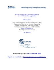
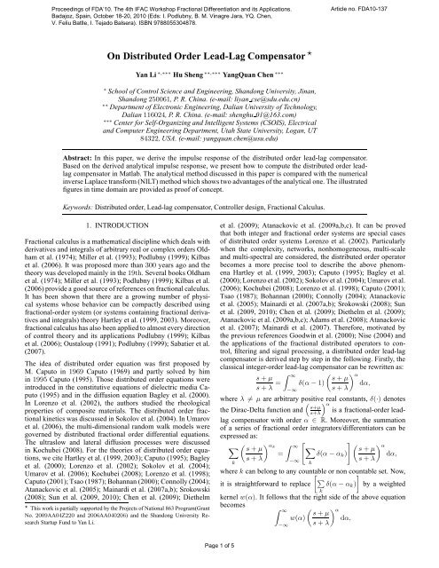
g 1 (t)<br />
0<br />
−0.05<br />
−0.1<br />
−0.15<br />
−0.2<br />
−0.25<br />
−0.3<br />
−0.35<br />
−0.4<br />
−0.45<br />
NILT<br />
Analytical Result<br />
−0.5<br />
0 1 2 3 4 5<br />
Time t<br />
6 7 8 9 10<br />
Fig. 1. The plots of g1(t) using (6) and NILT.<br />
L −1 {g2(s)} = 1<br />
s+γ<br />
st ( s + e<br />
2πi lo up<br />
)b − ( s+γ<br />
ln( s+γ<br />
s )<br />
γ<br />
e<br />
=<br />
−xt<br />
<br />
+ π2 <br />
0<br />
π ln 2 γ−x<br />
x<br />
a<br />
s )a<br />
γ b <br />
<br />
− x<br />
γ − x<br />
·<br />
−π cos(bπ) + sin(bπ)ln<br />
x<br />
x<br />
a <br />
<br />
γ − x<br />
γ − x<br />
−<br />
−π cos(aπ) + sin(aπ)ln dx.<br />
x<br />
x<br />
(7)<br />
Theorem 1. The inverse Laplace transform of <br />
b<br />
α<br />
s+µ<br />
a s+λ dα can<br />
be expressed as:<br />
L −1<br />
b <br />
α −µt −1 s + µ e L {g1(s)} , (λ > µ),<br />
dα =<br />
s + λ e −λt L −1 {g2(s)} , (λ < µ),<br />
where L −1 {g1(s)} and L −1 {g2(s)} are shown in equations (6)<br />
and (7), respectively.<br />
4. IMPLEMENTATION OF THE DISTRIBUTED ORDER<br />
LEAD-LAG COMPENSATOR<br />
In this Section, two distributed order lead-lag compensators are<br />
illustrated as the proof of concept. The analytical results derived<br />
in this paper are compared with the numerical inverse Laplace<br />
transform (NILT) algorithm Brancik (1999, 2001), where the<br />
“quadgk” function in Matlab is applied to compute the finite<br />
integral.<br />
L −1 {g1(s)} = 1<br />
s (<br />
st s+γ<br />
+ e<br />
2πi lo up<br />
)b − ( s<br />
s+γ )a<br />
ln( s<br />
s+γ )<br />
ds<br />
γ<br />
e<br />
=<br />
0<br />
−xt<br />
π Im<br />
<br />
xbe−ibπ (γ − x) −b − xae−iaπ (γ − x) −a<br />
ln( x<br />
<br />
dx<br />
γ−x ) − iπ<br />
γ<br />
e<br />
=<br />
0<br />
−xt<br />
<br />
π ln 2 <br />
x<br />
γ−x + π2 Let<br />
0.9 α s<br />
g1(s) =<br />
dα,<br />
0.1 s + 1<br />
we have<br />
g1(t) = L<br />
<br />
b <br />
<br />
x<br />
x<br />
· π cos(bπ) − sin(bπ)ln<br />
γ − x<br />
γ − x<br />
a <br />
<br />
x<br />
x<br />
− π cos(aπ) − sin(aπ)ln dx,<br />
γ − x<br />
γ − x<br />
(6)<br />
−1 {g1(s)}<br />
1<br />
e<br />
=<br />
0<br />
−xt<br />
<br />
π ln 2 <br />
x<br />
1−x + π2 <br />
0.9 <br />
<br />
x<br />
x<br />
·<br />
π cos(0.9π) − sin(0.9π)ln<br />
1 − x<br />
1 − x<br />
0.1 <br />
<br />
x<br />
x<br />
− π cos(0.1π) − sin(0.1π)ln<br />
1 − x<br />
1 − x<br />
<br />
dx.<br />
Page 3 of 5<br />
The plot of g1(t) is shown in Figure 1.<br />
Moreover, let<br />
0.9 α s + 1<br />
g2(s) =<br />
dα,<br />
s<br />
0.1<br />
ds
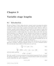
g 2 (t)<br />
0.5<br />
0.45<br />
0.4<br />
0.35<br />
0.3<br />
0.25<br />
0.2<br />
0.15<br />
0.1<br />
0.05<br />
NILT<br />
Analytical Result<br />
0<br />
0 1 2 3 4 5<br />
Time t<br />
6 7 8 9 10<br />
Fig. 2. The plots of g2(t) using (7) and NILT.<br />
it can be proved that<br />
g2(t) = L −1 {g2(s)}<br />
1<br />
e<br />
=<br />
0<br />
−(1−x)t<br />
<br />
π ln 2 <br />
x<br />
1−x + π2 <br />
0.9 <br />
<br />
x<br />
x<br />
·<br />
−π cos(0.9π) + sin(0.9π)ln<br />
1 − x<br />
1 − x<br />
0.1 <br />
<br />
x<br />
x<br />
−<br />
−π cos(0.1π) + sin(0.1π)ln<br />
1 − x<br />
1 − x<br />
<br />
dx,<br />
where the commutation law of convolution is applied in the above<br />
equation. The plot of g2(t) is shown in Figure 2.<br />
Remark 2. In the above two cases, the intervals of the integrals<br />
are [0.1, 0.9], which show that the discussed algorithm is applicable<br />
for all 0 ≤ a ≤ b ≤ 1. Therefore, our discussion can be<br />
extended to the whole time domain, i.e. −∞ < a < b < ∞.<br />
Remark 3. It can be seen from the above two figures that the<br />
analytical results derived in this paper can accurately compute<br />
the values of the two distributed order lead-lag compensators.<br />
Moreover, there are two features of the analytical results:<br />
• The convergence speed of the finite integral is getting faster<br />
for large t.<br />
• The impulse response can be computed accurately on the<br />
whole time domain.<br />
5. CONCLUSIONS AND FUTURE WORKS<br />
In this paper, we derived the impulse response of the distributed<br />
order lead-lag compensator. Based on the derived analytical impulse<br />
response, we presented how to compute the distributed<br />
order lead-lag compensator in Matlab. The method discussed<br />
in this paper was compared with the numerical inverse Laplace<br />
transform (NILT) method. It was shown that the convergence<br />
speed of the finite integral is getting faster for large t and the<br />
initial value can be computed accurately. The illustrated figures<br />
in time domain were provided as proof of concept.<br />
Our future works include the discretization of the distributed order<br />
lead-lag compensator and its applications to signal processing<br />
and control.<br />
ACKNOWLEDGEMENTS<br />
The authors would like to thank the chairs and reviewers for their<br />
valuable comments to improve this paper.<br />
Page 4 of 5<br />
REFERENCES<br />
K. B. Oldham and J. Spanier. The Fractional Calculus. Academic<br />
Press, New York, 1974.<br />
K. S. Miller and B. Ross. An Introduction to the Fractional<br />
Calculus and Fractional Differential Equations. Wiley, New<br />
York, 1993.<br />
Igor Podlubny. Fractional Differential Equations. Academic<br />
Press, 1999.<br />
A. A. Kilbas, H. M. Srivastava, and J. J. Trujillo. Theory and<br />
Applications of Fractional Differential Equations, Volume 204.<br />
Elsevier Science Inc., New York, NY, USA, 2006.<br />
Tom T. Hartley and Carl F. Lorenzo. Fractional system identification:<br />
An approach using continuous order-distributions. NASA<br />
Technical Memorandum, 209640:20 (pp), 1999.<br />
Tom T. Hartley and Carl F. Lorenzo. Fractional-order system<br />
identification based on continuous order-distributions. Signal<br />
Processing, 83(11):2287–2300, 2003.<br />
A. Oustaloup. La commande CRONE (in French). Hermès, Paris,<br />
France, 1991.<br />
I. Podlubny. Fractional-order systems and PI λ D µ -controllers.<br />
IEEE Transactions on Automatic Control, 44(1):208–214, January<br />
1999.<br />
J. Sabatier, O. P. Agrawal, and J. A. Tenreiro Machado. Advances<br />
in Fractional Calculus–Theoretical Developments and Applications<br />
in Physics and Engineering. Springer, 2007.<br />
M. Caputo. Elasticit ` da e dissipazione. Zanichelli, Bologna,<br />
1969.<br />
Michele Caputo. Mean fractional order derivatives differential<br />
equations and filters. Annali dell’Universita di Ferrara,<br />
41(1):73–84, 1995.<br />
R. L. Bagley and P. J. Torvik. <strong>On</strong> the existence of the order<br />
domain and the solution of distributed order equations (Parts<br />
I, II). International Journal of Applied Mechanics, 2:865–<br />
882,965–987, 2000.<br />
Carl F. Lorenzo and Tom T. Hartley. Variable order and distributed<br />
order fractional operators. Nonlinear Dynamics, 29(1–<br />
4):57–98, 2002.<br />
I. M. Sokolov, A. V. Chechkin, and J. Klafter. <strong>Distributed</strong>-order<br />
fractional kinetics. http://www.citebase.org/abstract?id<br />
=oai:arXiv.org:cond-mat/0401146, 2004.<br />
Sabir Umarov and Stanly Steinberg. Random walk models associated<br />
with distributed fractional order differential equations.<br />
Lecture Notes-Monograph Series, 51:117–127, 2006.<br />
Anatoly N. Kochubei. <strong>Distributed</strong> order calculus and equations<br />
of ultraslow diffusion. Journal of Mathematical Analysis and<br />
Applications, 340(1):252–281, 2008.<br />
Carl F. Lorenzo and Tom T. Hartley. Initialization, conceptualization,<br />
and application in the generalized fractional calculus.<br />
NASA technical paper, 208415:116 (pp), 1998.<br />
M. Caputo. <strong>Distributed</strong> order differential equations modelling<br />
dielectric induction and diffusion. Fractional Calculus &<br />
Applied Analysis, 4(4):421–442, 2001.<br />
Yuan Ying Tsao. Fractal concepts in the analysis of dispersion<br />
or relaxation processes. Thesis, Drexel University, June 1987.<br />
Gary Bohannan. Application of fractional calculus to polarization<br />
dynamics in solid dielectric materials. Thesis, Montana<br />
State University, November 2000.<br />
Joseph Arthur Connolly. The numerical solution of fractional and<br />
distributed order differential equations. Thesis, University of<br />
Liverpool, December 2004.<br />
T. M. Atanackovic, M. Budincevic, and S. Pilipovic. <strong>On</strong> a<br />
fractional distributed-order oscillator. Journal of Physics A:
Mathematical and General, 38(30):6703–6713, 2005.<br />
Francesco Mainardi, Antonio Mura, Rudolf Gorenflo, and Mirjana<br />
Stojanovic. The two forms of fractional relaxation of<br />
distributed order. Journal of Vibration and Control, 9:1249–<br />
1268, 2007a.<br />
G. C. Goodwin, S. F. Graebe and M. E. Salgado. Control System<br />
Design (1st.). Prentice Hall PTR, 2000.<br />
Norman S. Nise. Control Systems Engineering (4 ed.). Wiley &<br />
Sons, 2004.<br />
Francesco Mainardi and Gianni Pagnini. The role of the Fox-<br />
Wright functions in fractional sub-diffusion of distributed order.<br />
Journal of Computational and Applied Mathematics,<br />
207(2):245–257, 2007b.<br />
Tomasz Srokowski. Lévy flights in nonhomogeneous media:<br />
<strong>Distributed</strong>-order fractional equation approach. Phys. Rev. E,<br />
78(3):031135, Sep. 2008.<br />
H. G. Sun, W. Chen, and Y. Q. Chen. Variable-order fractional<br />
differential operators in anomalous diffusion modeling.<br />
Physica A: Statistical Mechanics and its Applications,<br />
388(21):4586–4592, 2009.<br />
HongGuang Sun, Wen Chen, Hu Sheng, and YangQuan Chen. <strong>On</strong><br />
mean square displacement behaviors of anomalous diffusions<br />
with variable and random orders. Physics Letters A, 374:906–<br />
910, 2010.<br />
Wen Chen, Hongguang Sun, Xiaodi Zhang, and Dean Korosak.<br />
Anomalous diffusion modeling by fractal and fractional<br />
derivatives. Computers & Mathematics with Applications,<br />
(DOI: 10.1016j.camwa.2009.08.020), In Press, Corrected<br />
Proof, 2009.<br />
Kai Diethelm and Neville J. Ford. Numerical analysis for<br />
distributed-order differential equations. Journal of Computational<br />
and Applied Mathematics, 225(1):96–104, 2009.<br />
Teodor M. Atanackovic, Stevan Pilipovic, and Dusan Zorica.<br />
Time distributed-order diffusion-wave equation. I. Volterratype<br />
equation. Proceedings of the Royal Society A, 465:1869–<br />
1891, 2009.<br />
Teodor M. Atanackovic, Stevan Pilipovic, and Dusan Zorica.<br />
Time distributed-order diffusion-wave equation. II. Applications<br />
of Laplace and Fourier transformations. Proceedings of<br />
the Royal Society A, 465:1893–1917, 2009.<br />
T. M. Atanackovic, S. Pilipovic, and D Zorica. Existence and calculation<br />
of the solution to the time distributed order diffusion<br />
equation. Physica Scripta, T136:014012 (6pp), 2009.<br />
J. L. Adams, T. T. Hartley, and C. F. Lorenzo. Identification of<br />
complex order-distributions. Journal of Vibration and Control,<br />
14(9-10):1375–1388, 2008.<br />
Teodor M. Atanackovic, Ljubica Oparnica, and Stevan Pilipovic.<br />
<strong>On</strong> a nonlinear distributed order fractional differential equation.<br />
Journal of Mathematical Analysis and Applications,<br />
328(1):590–608, 2007.<br />
Francesco Mainardi, Antonio Mura, Gianni Pagnini, and Rudolf<br />
Gorenflo. Time-fractional diffusion of distributed order.<br />
http://www.citebase.org/abstract?id=oai:arXiv.org:<br />
cond-mat/0701132, 2007.<br />
Brian Davies. Integral transforms and their applications (Third<br />
ed.). New York: Springer, 2002.<br />
Mingyu Xu and Wenchang Tan. Intermediate processes and<br />
critical phenomena: Theory, method and progress of fractional<br />
operators and their applications to modern mechanics. Science<br />
in China: Series G Physics, Mechanics and Astronomy,<br />
49(3):257–272, 2006.<br />
YangQuan Chen and Kevin L. Moore. Analytical stability bound<br />
for a class of delayed fractional order dynamic systems. Non-<br />
Page 5 of 5<br />
linear Dynamics, 29:191–200, 2002.<br />
Igor Podlubny. Geometric and physical interpretation of fractional<br />
integration and fractional differentiation. Fractional<br />
Calculus and Applied Analysis, 5(4):367–386, 2002.<br />
Igor Podlubny and Nicole Heymans. Physical interpretation<br />
of initial conditions for fractional differential equations with<br />
Riemann-Liouville fractional derivatives. Rheologica Acta,<br />
45(5):765–772, June 2006.<br />
L. Brančík. Programs for fast numerical inversion of Laplace<br />
transforms in MATLAB language environment. In Proceedings<br />
of the 7th Conference MATLAB99, Czech Republic,<br />
Prague., pages 27–39, 1999.<br />
L. Brančík. Programs for fast numerical inversion of Laplace<br />
transforms in MATLAB language environment. In Proceedings<br />
of the 11th International Czech-Slovak Scientific Conference<br />
Radioelektronika, Czech Republic, Brno., pages 352–355,<br />
2001.