16.1 The Kronig-Penny Model

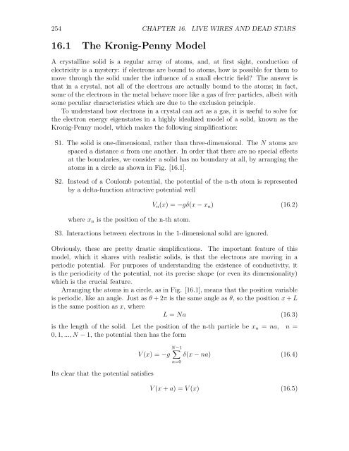
254 CHAPTER 16. LIVE WIRES AND DEAD STARS
16.1 The Kronig-Penny Model
A crystalline solid is a regular array of atoms, and, at first sight, conduction of
electricity is a mystery: if electrons are bound to atoms, how is possible for them to
move through the solid under the influence of a small electric field? The answer is
that in a crystal, not all of the electrons are actually bound to the atoms; in fact,
some of the electrons in the metal behave more like a gas of free particles, albeit with
some peculiar characteristics which are due to the exclusion principle.
To understand how electrons in a crystal can act as a gas, it is useful to solve for
the electron energy eigenstates in a highly idealized model of a solid, known as the
Kronig-Penny model, which makes the following simplifications:
S1. The solid is one-dimensional, rather than three-dimensional. The N atoms are
spaced a distance a from one another. In order that there are no special effects
at the boundaries, we consider a solid has no boundary at all, by arranging the
atoms in a circle as shown in Fig. [16.1].
S2. Instead of a Coulomb potential, the potential of the n-th atom is represented
by a delta-function attractive potential well
where xn is the position of the n-th atom.
Vn(x) = −gδ(x − xn) (16.2)
S3. Interactions between electrons in the 1-dimensional solid are ignored.
Obviously, these are pretty drastic simplifications. The important feature of this
model, which it shares with realistic solids, is that the electrons are moving in a
periodic potential. For purposes of understanding the existence of conductivity, it
is the periodicity of the potential, not its precise shape (or even its dimensionality)
which is the crucial feature.
Arranging the atoms in a circle, as in Fig. [16.1], means that the position variable
is periodic, like an angle. Just as θ + 2π is the same angle as θ, so the position x + L
is the same position as x, where
L = Na (16.3)
is the length of the solid. Let the position of the n-th particle be xn = na, n =
0, 1, ..., N − 1, the potential then has the form
Its clear that the potential satisfies
N−1
V (x) = −g δ(x − na) (16.4)
n=0
V (x + a) = V (x) (16.5)

16.1. THE KRONIG-PENNY MODEL 255
providing that we impose the periodicity requirement that x + L denotes the same
point as x. The “periodic delta-function” which incorporates this requirement is given
by
δ(x) = 1
exp [2πimx/L] (16.6)
2π m
The time-independent Schrodinger equation for the motion of any one electron in this
potential has the usual form
Hψk(x) = − ¯h2 ∂
2m
2
N−1
− g δ(x − na) ψk(x) = Ekψk(x) (16.7)
∂x2 n=0
Because V (x) has the symmetry (16.5), it is useful to consider the translation
operator first introduced in Chapter 10,
Likewise,
Taf(x) = exp[ia˜p/¯h]f(x)
= f(x + a) (16.8)
T−af(x) = exp[−ia˜p/¯h]f(x)
= f(x − a) (16.9)
Because ˜p is an Hermitian operator, its easy to see (just expand the exponentials in
a power series) that
T † a = T−a
[Ta, T−a] = 0
T−aTa = 1 (16.10)
Due to the periodicity of the potential V (x), the Hamiltonian commutes with the
translation operators, which, as we’ve seen, also commute with each other, i.e.
[Ta, H] = [T−a, H] = [Ta, T−a] = 0 (16.11)
This means (see Chapter 10) that we can choose energy eigenstates to also be eigenstates
of T±a, i.e.
Therefore,
TaψE(x) = λEψE(x)
T−aψE(x) = λ ′ E ψE(x) (16.12)
λE = < ψE|Ta|ψE >
= < T † a ψE|ψE >
= < T−aψE|ψE >
= (λ ′ E) ∗
(16.13)

256 CHAPTER 16. LIVE WIRES AND DEAD STARS
But also
ψE(x) = TaT−aψE
= λEλ ′ EψE
= ψE(x) (16.14)
This means that λ ′ E = (λE) −1 . Insert that fact into (16.13) and we conclude that
λ ∗ E = (λE) −1 , i.e.
λE = exp(iKa) (16.15)
for some K. In this way we arrive at
Bloch’s Theorem
For potentials with the periodicity property V (x + a) = V (x), each energy eigenstate
of the Schrodinger equation satisfies
for some value of K.
ψ(x + a) = e iKa ψ(x) (16.16)
It is also easy to work out the possible values of K, from the fact that
which implies
ψ(x) = ψ(x + L)
= (Ta) N ψ(x)
= exp[iNKa]ψ(x) (16.17)
K = 2π
j
Na
j = 0, 1, 2, ..., N − 1 (16.18)
The limiting value of j is N − 1, simply because
exp[i2π
j + N j
] = exp[i2π ] (16.19)
N N
so j ≥ N doesn’t lead to any further eigenvalues (j and N − j are equivalent).
According to Bloch’s theorem, if we can solve for the energy eigenstates in the
region 0 ≤ x ≤ a, then we have also solved for the wavefunction at all other values of
x. Now the periodic delta function potential V (x) vanishes in the region 0 < x < a,
so in this region (call it region I) the solution must have the free-particle form
ψI(x) = A sin(kx) + B cos(kx) E = ¯h2 k 2
2m
(16.20)

16.1. THE KRONIG-PENNY MODEL 257
But according to Bloch’s theorem, in the region −a < x < 0 (region II),
ψII(x) = e −iKa ψI(x + a)
= e −iKa [A sin k(x + a) + B cosk(x + a)] (16.21)
Now we apply continuity of the wavefunction at x = 0 to get
B = e −iKa [A sin(ka) + B cos(kb)] (16.22)
For a delta function potential, we found last semester a discontinuity in the slope of
the wavefunction at the location (x = 0) of the delta function spike, namely
and this condition gives us
Solving eq. (16.22) for A,
dψ
−
dx |ǫ
dψ
dx |−ǫ
= − 2mg
2 ψ(0) (16.23)
¯h
kA − e −iKa k[A cos(ka) − B sin(ka)] = − 2mg
2 B (16.24)
¯h
A = eiKa − cos(ka)
B (16.25)
sin(ka)
inserting into eq. (16.24) and cancelling B on both sides of the equation leads finally,
after a few manipulations, to
cos(Ka) = cos(ka) − mg
¯h 2 sin(ka) (16.26)
k
This equation determines the possible values of k, and thereby, via E = ¯h 2 k 2 /2m,
the possible energy eigenvalues of an electron in a periodic potential.
Now comes the interesting point. The parameter K can take on the values
2πn/Na, and cos(Ka) varies from cos(Ka) = +1 (n = 0) down to cos(Ka) = −1
(n = N/2), and back up to cos(Ka) ≈ +1 (n = N − 1). So the left hand side is
always in the range [−1, 1]. On the other hand, the right hand side is not always in
this range, and that means there are gaps in the allowed energies of an electron in a
periodic potential. This is shown in Fig. [16.2], where the right hand side of (16.26)
is plotted. Values of k for which the curve is outside the range [−1, 1] correspond
to regions of forbidden energies, known as energy gaps, while the values where the
curve is inside the [−1, 1] range correspond to allowed energies, known as energy
bands. The structure of bands and gaps is indicated in Fig. [16.3]; each of the
closely spaced horizontal lines is associated with a definite value of K.
In the case that we have M > N non-interacting electrons, each of the electrons
must be in an energy state corresponding to a line in one of the allowed energy bands.
The lowest energy state would naively be that of all electrons in the lowest energy

258 CHAPTER 16. LIVE WIRES AND DEAD STARS
level, but at this point we must invoke the Exclusion Principle: There can be no more
than one electron in any given quantum state. Thus there can a maximum of two
electrons (spin up and spin down) at any allowed energy in an energy band.
At the lowest possible temperature (T = 0 K), the electrons’ configuration is the
lowest possible energy consistent with the Exclusion Principle. A perfect Insulator
is a crystal in which the electrons completely fill one or more energy bands, and there
is a gap in energy from the most energetic electron to the next unoccupied energy
level. In a Conductor, the highest energy band containing electrons is only partially
filled.
In an applied electric field the electrons in a crystal will tend to accellerate, and
increase their energy. But...they can only increase their energy if there are (nearby)
higher energy states available, for electrons to occupy. If there are no nearby higher
energy states, as in an insulator, no current will flow (unless the applied field is so
enormous that electrons can ”jump” across the energy gap). In a conductor, there
are an enormous number of nearby energy states for electrons to move into. Electrons
are therefore free to accellerate, and a current flows through the material.
The actual physics of conduction, in a real solid, is of course far more complex
than this little calculation would indicate. Still, the Kronig-Penny model does a
remarkable job of isolating the essential effect, namely, the formation of separated
energy bands, which is due to the periodicity of the potential.
16.2 The Free Electron Gas
In the Kronig-Penney model, the electron wavefunctions have a free-particle form in
the interval between the atoms; there is just a discontinuity in slope at precisely the
position of the atoms. In passing to the three-dimensional case, we’ll simplify the
situation just a bit more, by ignoring even the discontinuity in slope. The electron
wavefunctions are then entirely of the free particle form, with only some boundary
conditions that need to be imposed at the surface of the solid. Tossing away the
atomic potential means losing the energy gaps; there is only one ”band,” whose
energies are determined entirely by the boundary conditions. For some purposes
(such as thermodynamics of solids, or computing the bulk modulus), this is not such
a terrible approximation.
We consider the case of N electrons in a cubical solid of length L on a side. Since
the electrons are constrained to stay within the solid, but we are otherwise ignoring
atomic potentials and inter-electron forces, the problem maps directly into a gas of
non-interacting electrons in a cubical box. Inside the box, the Schrodinger equation
for each electron has the free particle form
− ¯h2
2m ∇2 ψ(x, y, z) = Eψ(x, y, z) (16.27)