4 Coulomb blockade
4 Coulomb blockade
4 Coulomb blockade

Create successful ePaper yourself
Turn your PDF publications into a flip-book with our unique Google optimized e-Paper software.
4<br />
<strong>Coulomb</strong> <strong>blockade</strong><br />
Electron-electron interaction in nanosystems<br />
Single-electron box<br />
Single-electron transistor<br />
<strong>Coulomb</strong> <strong>blockade</strong> in quantum dots<br />
Cotunneling<br />
The effects of environment (to be written later)<br />
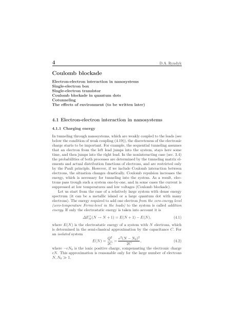
4.1 Electron-electron interaction in nanosystems<br />
4.1.1 Charging energy<br />
D.A. Ryndyk<br />
In tunneling through nanosystems, which are weakly coupled to the leads (see<br />
below the condition of weak coupling (4.19)), the discreteness of the electronic<br />
charge starts to be important. For example, the sequential tunneling assumes<br />
that an electron from the left lead jumps into the system, stays here some<br />
time, and then jumps into the right lead. In the noninteracting case (sec. 3.4)<br />
the probabilities of both processes are determined by the tunneling matrix elements<br />
and actual distribution functions of electrons, and are restricted only<br />
by the Pauli principle. However, if we include <strong>Coulomb</strong> interaction between<br />
electrons, the situation changes drastically. <strong>Coulomb</strong> repulsion increases the<br />
energy, which is necessary for tunneling into the system. As a result, electrons<br />
pass trough such a system one-by-one, and in some cases the current is<br />
suppressed at low temperatures and low voltages (<strong>Coulomb</strong> <strong>blockade</strong>).<br />
Let us start from the case of a relatively large system with dense energy<br />
spectrum (it can be a metallic island or a large quantum dot with many<br />
electrons). The energy required to add one electron from the zero-energy level<br />
(zero-temperature Fermi-level in the leads) to the system is called addition<br />
energy. If only the electrostatic energy is taken into account it is<br />
∆E +<br />
N (N → N +1)=E(N +1)−E(N), (4.1)<br />
where E(N) is the electrostatic energy of a system with N electrons, which<br />
is determined in the semi-classical approximation by the capacitance C. For<br />
an isolated system<br />
E(N) = Q2<br />
, (4.2)<br />
2C = e2 (N − N0) 2<br />
2C<br />
where −eN0 is the ionic positive charge, compensating the electronic charge<br />
eN. This approximation is reasonable only for the large number of electrons<br />
N,N0 ≫ 1.
68 4 <strong>Coulomb</strong> <strong>blockade</strong><br />
The minimal energy required to add one electron to the neutral system is<br />
called charging energy<br />
EC = ∆E +<br />
N0 (N0 → N0 +1)= e2<br />
. (4.3)<br />
2C<br />
If we want to add the second electron, the addition energy<br />
∆E +<br />
N0+1 (N0 +1→ N0 +2)= 3e2<br />
, (4.4)<br />
2C<br />
is required, and so on. We can say that in this case the discrete energy levels<br />
are formed by the <strong>Coulomb</strong> interaction, in spite of the fact that the initial<br />
energy spectrum is dense (quasi-continuous).<br />
The charging energy is an important energy scale. Let us estimate it in<br />
some typical cases. The classical expression for the capacitance of the usual<br />
oxide tunneling junction is C = εS/(4πd), where ε ≈ 10 is the dielectric constant<br />
of the oxide, S ≈ (100nm) 2 is the area of the junction, and d ≈ 10˚A is<br />
the thickness of the oxide layer. With these typical parameters the capacitance<br />
is C ≈ 10 −15 F, which corresponds to the charging energy EC ≈ 10 −4 eV and<br />
temperature T ∼ 1 K. This means that in metallic junctions the charging effects<br />
can be observed at sub-Kelvin temperatures. However, for nanoscale<br />
metallic particles, semiconductor quantum dots, and single molecules the<br />
charging energy, and corresponding temperature, can be orders of magnitude<br />
larger.<br />
4.1.2 Discrete energy levels<br />
The first important energy scale in small systems is the charging energy EC,<br />
the second one is the energy level spacing ∆ɛ between the eigenstates of a<br />
system. In metallic islands and semiconductor quantum dots the level spacing<br />
is determined by the geometrical size, because the discrete energy levels are<br />
formed as a result of spatial quantization of quasiparticles. It can be estimated<br />
using the free-electron expression near the Fermi surface. For example, in a<br />
3D system with characteristic size L<br />
∆ɛ(ɛF ) ∼ π2 ¯h 2<br />
, (4.5)<br />
mkF L3 here m is the effective mass, kF is the Fermi wave-vector.<br />
In smaller systems, like small quantum dots, multi quantum dot systems,<br />
and single molecules, the energy spectrum is more complex and the level<br />
spacing (or, more precisely, the energy spectrum ɛλ itself) should be calculated<br />
from the microscopic model. In this case the interactions can not be neglected<br />
and the level spacing ∆ɛ can not be unambiguously distinguished from the<br />
charging energy EC. In the limit of small single molecules the charging energy<br />
is, in fact, the same as the ionization energy, which in turn is related to
4.1 Electron-electron interaction in nanosystems 69<br />
the energy spectrum E(q, λ) of the isolated molecule, where q is the charge<br />
state, and λ is the eigenstate in this charge state. Finally, for nanosystems we<br />
understand the charging energy as the minimal energy required to add one<br />
electron to the neutral system, and the level spacing as the typical energy<br />
difference between two levels of the system in the same charge state.<br />
The consideration in this chapter is devoted mostly to the case of the dense<br />
energy spectrum ∆ɛ ≪ EC, when the directness of the energy levels can be<br />
neglected or taken into account within the simplified models.<br />
It is reasonable to note here, that the last very important energy scale is<br />
the temperature T . Both discrete energy spectrum and charging effects can<br />
be observed only if the temperature is lower, than the corresponding energy<br />
scales<br />
T ≪ ∆ɛ, T ≪ EC. (4.6)<br />
4.1.3 Anderson-Hubbard and constant-interaction models<br />
To take into account both discrete energy levels of a system and the electronelectron<br />
interaction, it is convenient to start from the general Hamiltonian<br />
ˆH = <br />
αβ<br />
˜ɛαβd † αdβ + 1<br />
2<br />
<br />
αβγδ<br />
Vαβ,γδd † αd †<br />
β dγdδ. (4.7)<br />
The first term of this Hamiltonian is a free-particle discrete-level model (2.8)<br />
with ˜ɛαβ including electrical potentials. And the second term describes all<br />
possible interactions between electrons and is equivalent to the real-space<br />
Hamiltonian<br />
ˆHee = 1<br />
<br />
2<br />
<br />
dξ<br />
where ˆ ψ(ξ) are field operators<br />
dξ ′ ˆ ψ † (ξ) ˆ ψ † (ξ ′ )V (ξ,ξ ′ ) ˆ ψ(ξ ′ ) ˆ ψ(ξ), (4.8)<br />
ˆψ(ξ) = <br />
ψα(ξ)dα, (4.9)<br />
α<br />
ψα(ξ) are the basis single-particle functions, we remind, that spin quantum<br />
numbers are included in α, and spin indices are included in ξ ≡ r,σ as variables.<br />
The matrix elements are defined as<br />
<br />
Vαβ,γδ = dξ dξ ′ ψ ∗ α(ξ)ψ ∗ β(ξ ′ )V (ξ,ξ ′ )ψγ(ξ)ψδ(ξ ′ ). (4.10)<br />
For pair <strong>Coulomb</strong> interaction V (|r|) the matrix elements are<br />
Vαβ,γδ = <br />
<br />
dr<br />
σσ ′<br />
dr ′ ψ ∗ α(r,σ)ψ ∗ β(r ′ ,σ ′ )V (|r − r ′ |)ψγ(r,σ)ψδ(r ′ ,σ ′ ).<br />
(4.11)
70 4 <strong>Coulomb</strong> <strong>blockade</strong><br />
Assume now, that the basis states |α〉 are the states with definite spin<br />
quantum number σα. It means, that only one spin component of the wave<br />
function, namely ψα(σα) is nonzero, and ψα(¯σα) = 0. In this case the only<br />
nonzero matrix elements are those with σα = σγ and σβ = σδ, theyare<br />
<br />
Vαβ,γδ = dr dr ′ ψ ∗ α(r)ψ ∗ β(r ′ )V (|r − r ′ |)ψγ(r)ψδ(r ′ ). (4.12)<br />
In the case of delocalized basis states ψα(r), the main matrix elements<br />
are those with α = γ and β = δ, because the wave functions of two different<br />
states with the same spin are orthogonal in real space and their contribution<br />
is small. It is also true for the systems with localized wave functions ψα(r),<br />
when the overlap between two different states is weak. In these cases it is<br />
enough to replace the interacting part by the Anderson-Hubbard Hamiltonian,<br />
describing only density-density interaction<br />
ˆHAH = 1 <br />
Uαβ ˆnαˆnβ. (4.13)<br />
2<br />
α=β<br />
with the Hubbard interaction defined as<br />
<br />
Uαβ = dr<br />
dr ′ |ψα(r)| 2 |ψβ(r ′ )| 2 V (|r − r ′ |). (4.14)<br />
In the limit of a single-level quantum dot (which is, however, a two-level<br />
system because of spin degeneration) we get the Anderson impurity model<br />
(AIM)<br />
ˆHAIM = <br />
σ=↑↓<br />
ɛσd † σdσ + U ˆn↑ˆn↓. (4.15)<br />
The other important limit is the constant interaction model (CIM), which<br />
is valid when many levels interact with similar energies, so that approximately,<br />
assuming Uαβ = U for any states α and β<br />
ˆHAH = 1 <br />
Uαβ ˆnαˆnβ ≈<br />
2<br />
α=β<br />
U<br />
2 <br />
ˆnα<br />
2<br />
α<br />
− U<br />
<br />
<br />
ˆn<br />
2<br />
α<br />
2 <br />
α<br />
= U ˆ N( ˆ N − 1)<br />
.<br />
2<br />
(4.16)<br />
where we used ˆn 2 =ˆn, forlargeNit is equivalent to (4.2).<br />
Thus, the CIM reproduces the charging energy considered above, and the<br />
Hamiltonian of an isolated system is<br />
ˆHCIM = <br />
αβ<br />
˜ɛαβd † αdβ + E(N). (4.17)<br />
Note, that the equilibrium compensating charge density can be easily introduced<br />
into the AH Hamiltonian<br />
ˆHAH = 1 <br />
Uαβ (ˆnα − ¯nα)(ˆnβ − ¯nβ) , (4.18)<br />
2<br />
α=β<br />
and at N ≫ 1 we obtain the electrostatic energy (4.2) with C = U/e 2 .
4.2 Single-electron box<br />
4.2 Single-electron box 71<br />
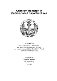
The simplest nanosystem, where the effects of single charge tunneling are important,<br />
is the single-electron box (SEB), a metallic island with dense electron<br />
spectrum coupled to the lead by a weak tunneling contact with the capacitance<br />
CL and the resistance RL (Fig. 4.1). Weak coupling means, that the<br />
tunneling resistance RT of the junction is rather high<br />
RT ≫ RK = h<br />
25.8 kΩ, (4.19)<br />
e2 the RK is a resistance quantum (it is defined only by the fundamental constants).<br />
Note, that this resistance is well known from the Landauer-Büttiker<br />
theory, where it plays the role of the minimum resistance of a single quantum<br />
channel. Thus, we understand now better the limits of weak (RT ≫ RK) and<br />
strong (RT ≤ RK) tunneling.<br />
We allow also to apply some voltage VGL to the system through the gate<br />
capacitance CG. The circuit is broken in this place, and the current can not<br />
flow though a system. The gate capacitance CG is ”true” capacitance, while<br />
the tunnel junction includes the classical capacitance CL and quantum ”possibility<br />
to tunnel” (shown by the cross). It is not equivalent to a classical<br />
resistance, in particular, the finite voltage at the capacitance CL does not<br />
imply necessarily the current through the tunnel junction.<br />
Now let us consider the following question: what is the charge state of the<br />
SEB at arbitrary voltage VGL? The important point is, that if the condition<br />
(4.19) is satisfied, the probability of tunneling is small, and electrons can<br />
be considered as localized inside the system almost all time. Therefore, the<br />
electronic charge of the SEB is quantized and is always en with integer n.<br />
However, the voltage VGL is arbitrary and tries to charge the capacitance by<br />
the charge CGVGL, which is not possible in general. The solution, found by<br />
L<br />
CLRL VGL<br />
System<br />
Gate<br />
CG<br />
CLRL VGL<br />
System<br />
Fig. 4.1. A single-electron box and its electrical scheme.<br />
CG
72 4 <strong>Coulomb</strong> <strong>blockade</strong><br />
the system, is to create two charges: QL at the capacitance of the tunneling<br />
contact and QG at the gate capacitance, in such a way that<br />
QL + QG = en,<br />
and the voltage is also divided between capacitances as<br />
VGL = QL<br />
−<br />
CL<br />
QG<br />
.<br />
CG<br />
From these two equations the charges QL and QG are easily defined as<br />
QL = CLCG<br />
CL + CG<br />
QG = CLCG<br />
CL + CG<br />
<br />
en<br />
+ VGL , (4.20)<br />
CG<br />
<br />
en<br />
. (4.21)<br />
− VGL<br />
CL<br />
Now we need the free energy of the system as a function of the electron<br />
number n with the gate voltage VGL as an external parameter. It allows to<br />
determine the ground state, and the probabilities of the states with different<br />
n, which are given by the Gibbs distribution. The problem is, that when<br />
the charge en is changed, the charges QL and QG are also changed and the<br />
external source makes the work −VGLdQG, notethatheretheasymmetry<br />
between true capacitance CG and the junction capacitance CL plays the role.<br />
After the Legendre transformation the free energy E ∗ (n) is<br />
E * (n)/E C<br />
n=0 n=1 n=2<br />
-1 0 1 2 3<br />
Q /|e|<br />
*<br />
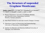
Fig. 4.2. The electrostatic energy E(n) of a single-electron box as a function of the<br />
gate voltage for the states with different number n of excess electrons. The thick<br />
line shows the states with minimum energy.
4.2 Single-electron box 73<br />
E ∗ (n) = Q2L +<br />
2CL<br />
Q2G + QGVGL, (4.22)<br />
2CG<br />
where C = CL + CG. Substituting (4.20) and (4.21) in this expression, we<br />
obtain<br />
E ∗ (n) = (en)2 CGVGL<br />
+<br />
2C C (en)+CLCGV 2 GL<br />
. (4.23)<br />
2C<br />
Neglecting the last irrelevant term independent on n, we get the free electrostatic<br />
energy of a SEB with n = N − N0 excess electrons:<br />
E ∗ (n) = e2 (n + Q∗ /e) 2<br />
, (4.24)<br />
2C<br />
where Q ∗ = CGVGL is determined by the gate voltage and is non-integer in<br />
the units of the elementary charge e.<br />
This expression can be obtained alternatively from the simple argument,<br />
that the full energy of the system is the sum of its own electrostatic energy and<br />
the energy of the charge ne in the external potential. Indeed, the first term in<br />
the formula (4.23) is the electrostatic energy of the isolated system, and the<br />
second term is the electrostatic energy in the external potential (CG/C)VGL in<br />
relation to the potential of the left lead. The full potential difference (voltage<br />
VLS) between the system and the left lead is (from (4.20))<br />
VLS = QL CGVGL<br />
+ , (4.25)<br />
CL<br />
C<br />
where the first term is the electrical potential produced by the charge of the<br />
island with capacitance C, and the second term is produced by the external<br />
voltage. Integrating it over the charge ne we obtain the free energy (4.23).<br />
We plot the energy E∗ (n) as a function of the gate charge Q∗ at different n<br />
(thenegativeelectronchargee = −|e| is taken into account explicitly) in the<br />
Fig. 4.2. This picture shows, that the state with minimal energy is changed<br />
with Q∗ . The neutral state n = 0 is stable at −0.5
74 4 <strong>Coulomb</strong> <strong>blockade</strong><br />
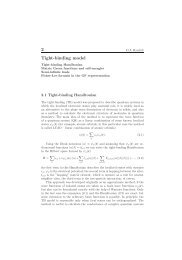
The average number of electrons is<br />
〈n〉 = <br />
np(n) = 1 <br />
<br />
n exp −<br />
Z<br />
E∗ <br />
(n)<br />
. (4.28)<br />
T<br />
n<br />
The results of calculation at different temperatures are shown in Fig. 4.3.<br />
We see, quite obviously, that the steps are smeared with temperature and<br />
disappear almost completely at T ≈ EC, in agreement with the estimate<br />
(4.6).<br />
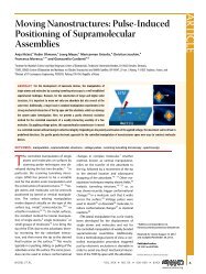
4.3 Single-electron transistor<br />
Now we come back to a transport problem. Consider the system between two<br />
leads coupled by two weak tunneling contacts (Fig. 4.4). When there is also<br />
the third electrode (gate), the system is called single-electron transistor.<br />
The electrostatic energy of the central region is given by the same formula<br />
(4.24) with the gate charge Q ∗ determined by the combination of all voltages<br />
applied to a system and the full capacitance is<br />
n<br />
C = CG + CL + CR. (4.29)<br />
The addition energy to increase the number of electrons from n to n +1 is<br />
∆E + n (n → n +1)=E ∗ (n +1)− E ∗ (n) = e2<br />
C<br />
<br />
3<br />
2<br />
1<br />
0<br />
<br />
n + 1 Q∗<br />
+<br />
2 e<br />
-1 0 1 2 3<br />
Q /|e|<br />
*<br />
-1<br />
<br />
. (4.30)<br />
Fig. 4.3. The average number of electrons 〈n〉 in a single-electron box as a function<br />
of the gate voltage at different temperatures T = 0.01EC (steps), T = 0.1EC,<br />
T =0.3EC, T = EC (nearly linear).
4.3 Single-electron transistor 75<br />
At zero bias voltage the system is equivalent to the single-electron box<br />
with two contacts instead of one, and the minimum energy, as well as the<br />
average number of excess electrons, are defined in the same way. At finite bias<br />
voltage V = VL − VR the current flows through the system. To calculate this<br />
current we use the sequential tunneling approach and master equation, valid<br />
in the limit of weak system-to-lead coupling (see sec. 3.4). To describe the<br />
transport we should calculate the nonequilibrium probability p(n) of different<br />
states n, which is not described now by the Gibbs distribution as for the<br />
single-electron box. First of all, let us determine the transition rates in the<br />
sequential tunneling regime.<br />
4.3.1 Tunneling transition rates<br />
The transition rate is determined by the golden-rule expression. For example,<br />
the transition from the state |n〉 to the state |n +1〉 due to the coupling to<br />
the left lead, is determined by the full probability of tunneling of one electron<br />
from any state |k〉 in the left lead to any single-particle state |α〉:<br />
n+1 n<br />
ΓL = 2π<br />
¯h<br />
2π<br />
¯h<br />
<br />
<br />
n +1| ˆ <br />
2<br />
HTL|n δ(Ei − Ef) =<br />
<br />
|Vkα| 2 fk (1 − fα) δ(Eα + ∆E + n − Ek), (4.31)<br />
kα<br />
the sum here is over all electronic states |k〉 in the left lead and all singleparticle<br />
states |α〉 in the system in the sense of the constant-interaction model<br />
(4.17), ˆHTL is the part of the tunneling Hamiltonian describing coupling to<br />
the left lead. All single-particle states are assumed to be thermalized and incoherent.<br />
The Fermi distribution functions fk and (1 − fα) describe probability<br />
CL<br />
L System<br />
R<br />
Gate<br />
VG<br />
CR<br />
VL R V<br />
CG<br />
Fig. 4.4. A single-electron transistor.
76 4 <strong>Coulomb</strong> <strong>blockade</strong><br />
for the state |k〉 to be occupied, and for the state |α〉 to be unoccupied. In such<br />
a way we take into account that the state denoted as |n〉 is, in fact, a mixed<br />
state of many single-particle states. We assume also for simplicity that the<br />
energy relaxation time is fast enough and the distribution of particles inside<br />
the system is equilibrium (but not the distribution p(n) of the different charge<br />
states!).<br />
Analogously, the transition from the state |n〉 to the state |n − 1〉 is determined<br />
by the probability of tunneling of one electron from the state with n<br />
electrons to the left lead<br />
n−1 n<br />
ΓL = 2π<br />
¯h<br />
2π<br />
¯h<br />
<br />
<br />
n − 1| ˆ <br />
2<br />
HTL|n δ(Ei − Ef )=<br />
<br />
|Vkα| 2 fα (1 − fk) δ(Eα + ∆E + n−1 − Ek). (4.32)<br />
kα<br />
Changing to the energy integration, we obtain<br />
<br />
dE1 dE2ΓL(E1,E2)f 0 L(E1) 1 − f 0 S(E2) δ(E2 + ∆E + n − E1),<br />
(4.33)<br />
n+1 n<br />
ΓL =<br />
where<br />
Γi=L,R(E1,E2) = 2π<br />
¯h<br />
<br />
|Vα,ik| 2 δ(E1 − Eα)δ(E2 − Ek). (4.34)<br />
kα<br />
Further simplification is possible in the wide-band limit, assuming that<br />
Γi=L,R(E1,E2) is energy-independent. Finally, we arrive at<br />
where Gi is the tunneling conductance<br />
n+1 n<br />
Γi=L,R =(Gi/e 2 )f(∆E + n + eViS), (4.35)<br />
Gi=L,R = 4πe2<br />
¯h Ni(0)NS(0)|V | 2 , (4.36)<br />
with the densities of states Ni(0) and NS(0), and f(E) is<br />
E<br />
f(E) =<br />
exp . (4.37)<br />
E<br />
T − 1<br />
In the same way for the transition from n to n − 1weget<br />
Γ n−1 n<br />
i=L,R =(Gi/e 2 )f(−∆E + n−1 − eViS). (4.38)
4.3.2 Master equation<br />
4.3 Single-electron transistor 77<br />
Now we can write the classical master equation for the probability p(n, t) to<br />
find a state with n electrons<br />
dp(n, t)<br />
dt<br />
= Γ nn−1<br />
L + Γ nn−1<br />
nn+1<br />
R p(n − 1,t)+ ΓL + Γ nn+1<br />
R p(n +1,t)−<br />
n−1 n n+1 n n−1 n n+1 n<br />
ΓL + ΓL + ΓR + ΓR p(n, t), (4.39)<br />
where the transitions rates are calculated previously (4.35), (4.38). Introducing<br />
the short-hand notations<br />
we arrive at<br />
dp(n, t)<br />
dt<br />
Γ nn−1 = Γ nn−1<br />
L<br />
Γ nn+1 = Γ nn+1<br />
L<br />
+ Γ nn−1<br />
R ,<br />
+ Γ nn+1<br />
R ,<br />
= Γ nn−1 p(n − 1,t)+Γ nn+1 p(n +1,t) − Γ n−1 n + Γ n+1 n p(n, t).<br />
(4.40)<br />
The structure of this equation is completely clear. The first two terms describe<br />
transfer of one electron from the leads to the system (if the state before<br />
tunneling is |n − 1〉) or from the system to the leads (if the initial state is<br />
|n +1〉), in both cases the final state is |n〉, thus raising the probability p(n)<br />
to find this state. The last term in (4.40) describes tunneling from the state<br />
|n〉 into |n − 1〉 or |n +1〉.<br />
The current (from the left or right lead to the system) is<br />
Ji=L,R(t) =e <br />
n<br />
Γ n+1 n<br />
i<br />
− Γ<br />
n−1 n<br />
i<br />
p(n, t). (4.41)<br />
In the stationary case the solution of the master equation (4.40) is given<br />
by the recursive relation (which is actually the stationary balance equation<br />
between |n〉 and |n − 1〉 states).<br />
Γ n−1 n p(n) =Γ nn−1 p(n − 1). (4.42)<br />
It can be solved very easily numerically, one can start from an arbitrary value<br />
for one of the p(n), then calculate all other p(n) going up and down in n to<br />
some fixed limiting number, and, finally, normalize all the p(n) tosatisfythe<br />
condition (4.27).<br />
Below we present the numerical solution in two cases: for conductance in<br />
the limit of low voltage, and for the voltage-current curves. The transport is<br />
blocked at low temperature and low voltage because of the non-zero addition<br />
energy (4.30).
78 4 <strong>Coulomb</strong> <strong>blockade</strong><br />
G [arb. u.]<br />
-1 0 1 2 3<br />
Q /|e|<br />
*<br />
Fig. 4.5. Conductance oscillations as a function of the gate voltage at different<br />
temperatures T =0.01EC, T =0.1EC, T =0.3EC, T =0.5EC (upper curve).<br />
4.3.3 Conductance: CB oscillations<br />
Consider first the conductance of a system as a function of the gate voltage<br />
VG (gate charge Q ∗ ). The result is shown in Fig. 4.5. The conductance has<br />
maximum in the degeneracy points Q ∗ /|e| = n+0.5, when the addition energy<br />
(4.30) vanishes. Between these points the conductance is very small at low<br />
temperatures, because the electron can not overcome the <strong>Coulomb</strong> energy,<br />
the effect was nick-named ”<strong>Coulomb</strong> <strong>blockade</strong>”.<br />
The phenomena can be described within the noninteracting particle picture,<br />
if we notice, that the charging energy produce, in fact, discrete energy<br />
levels, while the gate voltage works as a potential changing the position of<br />
the levels up and down in energy. The maximum of the conductance is observed<br />
when this induced discrete level is in resonance with the Fermi levels<br />
in the leads. This single-particle picture (or better to say analogy), however,<br />
should be used with care. The problem is that this single-particle level is<br />
fictional and corresponds, in fact, to a superposition of two many-particle<br />
states with different number of electrons. In the degeneracy point the probabilities<br />
p(n) andp(n + 1) of the states with different number of electrons<br />
are equal. This circumstance shows that the <strong>Coulomb</strong> <strong>blockade</strong> is essentially<br />
many-particle phenomena, and the mean-field (Hartree-Fock) approximation<br />
can not be used to describe it. Later we shall see, that it is a consequence of<br />
the degeneracy of a single-particle spectrum.<br />
At higher temperatures, the oscillations are smeared and completely disappear<br />
at T ∼ EC, the effect is analogous to the charge quantization in a<br />
single-electron box.
J [arb. u.]<br />
4.3 Single-electron transistor 79<br />
0 1 2 3 4<br />
V<br />
Fig. 4.6. <strong>Coulomb</strong> <strong>blockade</strong>: voltage-current curves of a symmetric junction at low<br />
temperature (T =0.01EC) and different gate voltages VG =0,VG =0.25EC, and<br />
VG = 0.5EC. Dashed line shows the change at higher temperature T = 0.1EC.<br />
Voltage is in units of EC/|e|.<br />
4.3.4 Current-voltage curve: <strong>Coulomb</strong> staircase<br />
Now let us discuss the signatures of <strong>Coulomb</strong> <strong>blockade</strong> at finite voltage. The<br />
results of calculations are presented in Fig. 4.6 for symmetric (νL = νR) system,<br />
and in Fig. 4.7 for asymmetric one. First of all, the gap (called <strong>Coulomb</strong><br />
gap) is seen clear at low temperatures and low voltages, that is the other one<br />
manifestation of <strong>Coulomb</strong> <strong>blockade</strong>. In agreement with conductance calculation,<br />
this gap is closed in the degeneracy points, where the linear currentvoltage<br />
relation is reproduced at low voltages. At higher temperatures the<br />
gap is smeared and linear behaviour is restored.<br />
The other characteristic feature, seen at higher voltages and more pronounced<br />
in the asymmetric case, is called <strong>Coulomb</strong> staircase (Fig. 4.7) and<br />
is observed due to the participation of higher charge states in transport at<br />
higher voltage. For example, if VG = 0 the transport is blocked at low voltage<br />
and the current appears only at |e|V/2 >EC (V/2 because the bias voltage is<br />
divided between the left and right contacts) when the <strong>Coulomb</strong> gap is overcome<br />
and the electron can go through the state |n =1〉. At higher voltage<br />
|e|V/2 > 3EC the state |n =2〉 become available, and so on.<br />
The general formula for the threshold voltages of the n-th step is<br />
Vn = ±<br />
2(2n − 1)EC<br />
. (4.43)<br />
|e|<br />
The amplitude of the steps is decaying with n and at large voltage the Ohmic<br />
behaviour is reproduced.
80 4 <strong>Coulomb</strong> <strong>blockade</strong><br />
J [arb. u.]<br />
0 2 4 6 8<br />
V<br />
Fig. 4.7. <strong>Coulomb</strong> staircase: voltage-current curves of an asymmetric junction at<br />
low temperature (T =0.01EC) at different gate voltages VG =0,VG =0.25EC,<br />
and VG =0.5EC. Dashed line shows the change at higher temperature T =0.1EC.<br />
Voltage is in units of EC/|e|.<br />
4.3.5 Contour plots. Stability diagrams<br />
To analyze the experiments the contour plots of the current J(V,VG) (Fig. 4.8)<br />
and the differential conductance dJ/dV (V,VG) (Fig. 4.9) are very useful. The<br />
characteristic structures of <strong>Coulomb</strong> <strong>blockade</strong> (so-called <strong>Coulomb</strong> diamonds)<br />
are well pronounced in these pictures.<br />
The white rhombic-shaped regions are the regions of <strong>Coulomb</strong> <strong>blockade</strong>.<br />
At zero temperature there is no current, one state with n electrons is stable<br />
with respect to tunneling. For example, near the point V = VG = 0 the state<br />
n = 0 is stable. If one changes the gate voltage, the other charge states become<br />
stable. At large enough bias voltage the stability is lost and sequential tunneling<br />
events produce a finite current. The contour plots, as well as a schematic<br />
representations of the boundaries of the stability region in the (V,VG) plane,<br />
are often called stability diagrams.<br />
While both left and right tunneling events should be suppressed, there<br />
are two stability conditions, obtained directly from the tunneling rates (4.35),<br />
(4.38)<br />
<br />
|e| n − 1<br />
<br />
<br />
V<br />
4<br />
2<br />
0<br />
-2<br />
4.3 Single-electron transistor 81<br />
-4<br />
-2 -1 0<br />
VG 1 2<br />
Fig. 4.8. Contour plot of the current.<br />
where V = VL − VR is the bias voltage, and VGL = VG − VL, VGR = VG − VR<br />
are the voltages between the gate and the leads.<br />
These inequalities show that if the system leaves the stability region at<br />
finite bias voltage V , the new state with n = n ± 1, which occurs as a result<br />
of tunneling through one junction, is also unstable with respect to tunneling<br />
through the other junction. As a result, the systems returns back to the state<br />
n, and the cycle is started again, thus the current flows through the system.<br />
V<br />
4<br />
2<br />
0<br />
-2<br />
-4<br />
-2 -1 0<br />
VG 1 2<br />
Fig. 4.9. Contour plot of the differential conductance.<br />
1.2<br />
0.8<br />
0.4<br />
0<br />
-0.4<br />
-0.8<br />
-1.2<br />
0.3<br />
0.1<br />
0
82 4 <strong>Coulomb</strong> <strong>blockade</strong><br />
4.4 <strong>Coulomb</strong> <strong>blockade</strong> in quantum dots<br />
Here we want to consider the <strong>Coulomb</strong> <strong>blockade</strong> in intermediate-size quantum<br />
dots, where the typical energy level spacing ∆ɛ is not too small to neglect it<br />
completely, but the number of levels is large enough, so that one can use the<br />
constant-interaction model (4.17), which we write in the eigenstate basis as<br />
ˆHCIM = <br />
α<br />
˜ɛαd † αdα + E(n), (4.46)<br />
where the charging energy E(n) is determined in the same way as previously,<br />
for example by the expression (4.16). Note, that for quantum dots it is not<br />
convenient to incorporate the gate voltage into the free electrostatic energy<br />
(4.24), as we did before for metallic islands, also the usage of classical capacitance<br />
is not well established, although for large quantum dots it is possible.<br />
Instead, we shift the energy levels in the dot ˜ɛα = ɛα + eϕα by the electrical<br />
potential<br />
ϕα = VG + VR + ηα(VL − VR), (4.47)<br />
where ηα are some coefficients, dependent on geometry. This method can be<br />
easily extended to include any self-consistent effects on the mean-field level by<br />
the help of the Poisson equation (instead of classical capacitances). Besides,<br />
if all ηα are the same, our approach reproduce again the relevant part of the<br />
classical expressions (4.23), (4.24)<br />
ÊCIM = <br />
ɛαnα + E(n)+enϕext. (4.48)<br />
α<br />
The addition energy now depends not only on the charge of the molecule,<br />
but also on the state |α〉, in which the electron is added<br />
∆E + nα(n, nα =0→ n +1,nα =1)=E(n +1)− E(n)+ɛα, (4.49)<br />
we can assume in this case, that the single particle energies are additive to the<br />
charging energy, so that the full quantum eigenstate of the system is |n, ˆn〉,<br />
where the set ˆn ≡{nα} shows weather the particular single-particle state |α〉<br />
is empty or occupied. Some arbitrary state ˆn looks like<br />
ˆn ≡{nα} ≡ n1,n2,n3,n4,n5, ... = 1, 1, 0, 1, 0, ... . (4.50)<br />
Note, that the distribution ˆn defines also n = <br />
α nα. It is convenient, however,<br />
to keep notation n to remember about the charge state of a system,<br />
below we use both notations |n, ˆn〉 and short one |ˆn〉 as equivalent.<br />
The other important point is that the distribution function fn(α) inthe<br />
charge state |n〉 is not assumed to be equilibrium, as previously (this condition<br />
is not specific to quantum dots with discrete energy levels, the distribution<br />
function in metallic islands can also be nonequilibrium. However, in the parameter<br />
range, typical for classical <strong>Coulomb</strong> <strong>blockade</strong>, the tunneling time is
4.4 <strong>Coulomb</strong> <strong>blockade</strong> in quantum dots 83<br />
much smaller than the energy relaxation time, and quasiparticle nonequilibrium<br />
effects are usually neglected).<br />
With these new assumptions, the theory of sequential tunneling is quite<br />
the same, as was considered in the previous section. The master equation<br />
(4.40) is replaced by<br />
dp(n, ˆn, t)<br />
=<br />
dt<br />
<br />
ˆn ′<br />
nn−1<br />
Γˆnˆn ′ p(n − 1, ˆn ′ ,t)+Γ nn+1<br />
ˆnˆn ′ p(n +1, ˆn ′ ,t) −<br />
n−1 n<br />
Γˆn ′ n+1 n<br />
ˆn + Γˆn ′ <br />
ˆn p(n, ˆn, t)+I {p(n, ˆn, t)} , (4.51)<br />
ˆn ′<br />
where p(n, ˆn, t) is now the probability to find the system in the state |n, ˆn〉,<br />
Γ nn−1<br />
is the transition rate from the state with n−1 electrons and single level<br />
ˆnˆn ′<br />
occupation ˆn ′ into the state with n electrons and single level occupation ˆn.<br />
The sum is over all states ˆn ′ , which are different by one electron from the state<br />
ˆn. The last term is included to describe possible inelastic processes inside the<br />
system and relaxation to the equilibrium function peq(n, ˆn). In principle, it<br />
is not necessary to introduce such type of dissipation in calculation, because<br />
the current is in any case finite. But the dissipation may be important in<br />
large systems and at finite temperatures. Besides, it is necessary to describe<br />
the limit of classical single-electron transport, where the distribution function<br />
of qausi-particles is assumed to be equilibrium. Below we shall not take into<br />
account this term, assuming that tunneling is more important.<br />
While all considered processes are, in fact, single-particle tunneling pro-<br />
cesses, we arrive at<br />
dp(ˆn, t)<br />
=<br />
dt<br />
<br />
β<br />
<br />
δnβ1Γ<br />
δnβ1Γ nn−1<br />
β<br />
β<br />
p(ˆn, nβ =0,t)+δnβ0Γ nn+1<br />
<br />
β p(ˆn, nβ =1,t) −<br />
n−1 n<br />
β<br />
+ δnβ0Γ<br />
n+1 n<br />
β<br />
<br />
p(ˆn, t), (4.52)<br />
where the sum is over single-particle states. The probability p(ˆn, nβ =0,t)<br />
is the probability of the state equivalent to ˆn, but without the electron in<br />
the state β. Consider, for example, the first term in the right part. Here the<br />
delta-function δnβ1 shows, that this term should be taken into account only if<br />
the single-particle state β in the many-particle state ˆn is occupied, Γ nn−1<br />
β is<br />
the probability of tunneling from the lead to this state, p(ˆn, nβ =0,t)isthe<br />
probability of the state ˆn ′ , from which the system can come into the state ˆn.<br />
The transitions rates are defined by the same golden rule expressions, as<br />
before (4.31), (4.32), but with explicitly shown single-particle state α<br />
n+1 n 2π<br />
<br />
<br />
ΓLα = n +1,nα =1|<br />
¯h<br />
ˆ 2 <br />
HTL|n, nα =0 δ(Ei − Ef) =<br />
2π <br />
|Vkα|<br />
¯h<br />
2 fkδ(∆E + nα − Ek), (4.53)<br />
k
84 4 <strong>Coulomb</strong> <strong>blockade</strong><br />
n−1 n 2π<br />
<br />
<br />
ΓLα = n − 1,nα =0|<br />
¯h<br />
ˆ <br />
2<br />
HTL|n, nα =1 δ(Ei − Ef) =<br />
2π <br />
|Vkα|<br />
¯h<br />
k<br />
2 (1 − fk) δ(∆E + n−1 α − Ek), (4.54)<br />
there is no occupation factors (1 − fα), fα because this state is assumed to<br />
be empty in the sense of the master equation (4.52). The energy of the state<br />
is now included into the addition energy.<br />
Using again the level-width function<br />
Γi=L,R α(E) = 2π <br />
|Vik,α|<br />
¯h<br />
2 δ(E − Ek). (4.55)<br />
we obtain<br />
k<br />
n+1 n Γα = ΓLαf 0 L (∆E+ nα)+ΓRαf 0 R (∆E+ nα), (4.56)<br />
<br />
n−1 n<br />
0 Γα = ΓLα 1 − fL (∆E + n−1 α ) <br />
0 + ΓRα 1 − fR (∆E + n−1 α ) . (4.57)<br />
Finally, the current from the left or right contact to a system is<br />
Ji=L,R = e <br />
p(ˆn)Γiα δnα0f 0 i (∆E + nα) − δnα1(1 − f 0 i (∆E + nα)) . (4.58)<br />
α<br />
ˆn<br />
The sum over α takes into account all possible single particle tunneling events,<br />
the sum over states ˆn summarize probabilities p(ˆn) of these states.<br />
4.4.1 Linear conductance<br />
The linear conductance can be calculated analytically [25, 26]. Here we present<br />
the final result:<br />
G = e2<br />
T<br />
<br />
α<br />
∞<br />
ΓLαΓRα<br />
ΓLα + ΓRα<br />
n=1<br />
Peq(n, nα =1) 1 − f 0 (∆E + n−1 α ) , (4.59)<br />
where Peq(n, nα = 1) is the joint probability that the quantum dot contains<br />
n electrons and the level α is occupied<br />
Peq(n, nα =1)= <br />
⎛<br />
peq(ˆn)δ ⎝n − <br />
⎞<br />
⎠ δnα1, (4.60)<br />
ˆn<br />
and the equilibrium probability (distribution function) is determined by the<br />
Gibbs distribution in the grand canonical ensemble:<br />
peq(ˆn) = 1<br />
Z exp<br />
<br />
− 1<br />
<br />
<br />
˜ɛα + E(n) . (4.61)<br />
T<br />
α<br />
β<br />
nβ
G [arb. u.]<br />
4.4 <strong>Coulomb</strong> <strong>blockade</strong> in quantum dots 85<br />
-1 0 1 2 3<br />
V G<br />
Fig. 4.10. Linear conductance of a QD as a function of the gate voltage at different<br />
temperatures T =0.01EC, T =0.03EC, T =0.05EC, T =0.1EC, T =0.15EC<br />
(lower curve).<br />
A typical behaviour of the conductance as a function of the gate voltage<br />
at different temperatures is shown in Fig. 4.10. In the resonant tunneling<br />
regime at low temperatures T ≪ ∆ɛ the peak height is strongly<br />
temperature-dependent. It is changed by classical temperature dependence<br />
(constant height) at T ≫ ∆ɛ.<br />
4.4.2 Transport at finite bias voltage<br />
At finite bias voltage we find new manifestations of the interplay between<br />
single-electron tunneling and resonant free-particle tunneling.<br />
Now, let us consider current-voltage curve of the differential conductance<br />
(Fig. 4.12). First of all, <strong>Coulomb</strong> staircase is reproduced, which is more pronounced,<br />
than for metallic islands, because the density of states is limited by<br />
the available single-particle states and the current is saturated. Besides, small<br />
additional steps due to discrete energy levels appear. This characteristic behaviour<br />
is possible for large enough dots with ∆ɛ ≪ EC. If the level spacing<br />
is of the oder of the charging energy ∆ɛ ∼ EC, the <strong>Coulomb</strong> <strong>blockade</strong> steps<br />
and discrete-level steps look the same, but their statistics (position and height<br />
distribution) is determined by the details of the single-particle spectrum and<br />
interactions [27].<br />
Finally, let us consider the contour plot of the differential conductance<br />
(Fig. 4.12). Ii is essentially different from those for the metallic island<br />
(Fig. 4.9). First, it is not symmetric in the gate voltage, because the energy<br />
spectrum is restricted from the bottom, and at negative bias all the levels are
86 4 <strong>Coulomb</strong> <strong>blockade</strong><br />
J [arb. u.]<br />
V<br />
0 2 4 6 8<br />
V<br />
4<br />
2<br />
0<br />
-2<br />
Fig. 4.11. <strong>Coulomb</strong> staircase.<br />
-4<br />
-1 0 1<br />
VG 2 3<br />
Fig. 4.12. Contour plot of the differential conductance.<br />
above the Fermi-level (the electron charge is negative, and a negative potential<br />
means a positive energy shift). Nevertheless, existing stability patterns are of<br />
the same origin and form the same structure. The qualitatively new feature<br />
is additional lines correspondent to the additional discrete-level steps in the<br />
voltage-current curves.In general, the current and conductance of quantum<br />
dots demonstrate all typical features of discrete-level systems: current steps,<br />
conductance peaks. Without <strong>Coulomb</strong> interaction the usual picture of resonant<br />
tunneling is reproduced. In the limit of dense energy spectrum ∆ɛ → 0<br />
the sharp single-level steps are merged into the smooth <strong>Coulomb</strong> staircase.<br />
0.7<br />
0
4.5 Cotunneling<br />
4.5 Cotunneling 87<br />
Until now we have considered only the sequential tunneling regime, which is<br />
described by the first-order perturbation in tunneling. At low temperatures<br />
the sequential tunneling is suppressed by the <strong>Coulomb</strong> <strong>blockade</strong> (excepting<br />
the degeneracy points), and the conductance of the system become exponentially<br />
small. In this case the second-order processes start to be important.<br />
These processes include the events, when two electrons with different energy<br />
participate in tunneling simultaneously (so-called inelastic cotunneling), or<br />
one electron tunnels coherently twice (elastic cotunneling), which is equivalent,<br />
however, to the simultaneous tunneling of two electrons with the same<br />
energy. Note, that both terms ”inelastic” and ”elastic” have no relation to the<br />
presence or absence of the additional inelastic interactions inside the system.<br />
The standard second-order perturbation theory yields the transition rate<br />
from some initial state |i〉 to some final state |f〉<br />
Γ (2) 2π<br />
i→f =<br />
¯h<br />
<br />
<br />
<br />
f <br />
<br />
<br />
<br />
ˆHT<br />
<br />
<br />
λ λ ˆHT<br />
<br />
<br />
2<br />
i<br />
<br />
<br />
<br />
Eλ − Ei<br />
δ(Ei − Ef ). (4.62)<br />
<br />
λ<br />
Theintermediatestates|λ〉 are virtual states with Eλ >Ei. Inthispointwe<br />
already assume that the system is in the <strong>Coulomb</strong> <strong>blockade</strong> regime with fixed<br />
number of electrons n, and the temperature is low T ≪ ∆E + n , because in the<br />
opposite case thermally excited quasiparticles in the leads can overcome the<br />
energy barrier, and the sequential tunneling through high-energy states will<br />
determine the current.<br />
Fig. 4.13. Cotunneling processes, elastic (a,c) and inelastic (b,d).<br />
(from Aleiner et al.).
88 4 <strong>Coulomb</strong> <strong>blockade</strong><br />
Before considering the particular cases, let us perform all possible general<br />
calculations in (4.62). First of all, the tunneling Hamiltonian is the sum of<br />
left and right parts, we are interested only in the processes, which transfer<br />
electrons from the left to the right, and include one tunneling through the<br />
right junction and one tunneling through the left junction. Then, the initial<br />
state is a mixed state with different probabilities for the states |k〉 and |q〉 to be<br />
occupied or empty, following the tunneling theory we introduce the sum over<br />
all possible configurations of the initial state with corresponding occupation<br />
probabilities (distribution functions) f 0 L (Ek) andf 0 R (Eq). Thus, we obtain<br />
Γ (2) 2π<br />
L→R =<br />
¯h<br />
<br />
<br />
<br />
× <br />
<br />
<br />
λ<br />
fq<br />
<br />
k∈L,q∈R<br />
f 0 L(Ek) 1 − f 0 R(Eq) δ(Ei − Ef )<br />
<br />
<br />
ˆ <br />
<br />
HTR<br />
λ λ ˆ <br />
<br />
HTL<br />
ik<br />
<br />
+<br />
fq<br />
Eλ − Ei<br />
<br />
<br />
ˆ <br />
<br />
HTL<br />
λ λ ˆ <br />
<br />
HTR<br />
ik<br />
2<br />
<br />
<br />
<br />
. (4.63)<br />
<br />
The intermediate states |λ〉 are the states with one extra electron (or<br />
without one electron, e.g. with one extra hole) in the central system. Note,<br />
that the only thing we assume is that the charge of the central system is the<br />
same in the initial and the final states (and ±e in the virtual intermediate<br />
state). However the state and energy of the central system can change after<br />
tunneling event. In the last case the process is called inelastic cotunneling.<br />
Up to now, all our calculation is general, now it is reasonable to consider<br />
separately the contributions of inelastic and elastic cotunneling.<br />
4.5.1 Inelastic cotunneling<br />
Consider the final state as the state with one electron transferred from the<br />
state k in the left lead to the state q in the right lead with the change of the<br />
state of the system from |λi〉 with electron in the state α and empty state β<br />
to |λf 〉 with electron removed from α to β<br />
<br />
<br />
f = c † qckd †<br />
<br />
<br />
i , (4.64)<br />
the energy conservation implies that<br />
β dα<br />
Ei = Ek + Eα = Ef = Eq + Eβ. (4.65)<br />
Due to mutual incoherence of these states, not the amplitudes, but the<br />
probabilities of different events should be summarized. Below we neglect all<br />
cross-terms with different indices λ, and apply<br />
<br />
<br />
<br />
<br />
Xλ<br />
2<br />
= |Xλ| 2 . (4.66)
4.5 Cotunneling 89<br />
In the metallic dots we can assume that the distribution over internal<br />
single-particle states is equilibrium, and obtain<br />
Γ (2)n<br />
in<br />
2π<br />
=<br />
¯h<br />
<br />
k∈L,q∈R αβ<br />
<br />
1<br />
Eβ + ∆E + +<br />
n − Ek<br />
1<br />
Eq − ∆E + n−1 − Eα<br />
2<br />
|Vαq| 2 |Vβk| 2<br />
× f 0 L(Ek) 1 − f 0 R(Eq) 1 − f 0 S(Eβ) f 0 S(Eα)δ(Ek + Eα − Eq − Eβ). (4.67)<br />
The two terms in this expression correspond to two physical processes. The<br />
first one describes the jump (virtual!) of the extra electron from the state k in<br />
the left lead into the state β in the system, and then the other electron jumps<br />
through the second junction from the state α into the state q in the right<br />
lead (Fig. 4.13b). In the second process (Fig. 4.13d) first the electron jumps<br />
from the system into the right lead, and then the second electron jumps from<br />
the left lead. All other matrix elements of the tunneling Hamiltonians in the<br />
expression (4.63) are zero. The distribution functions describe as usually the<br />
probabilities of necessary occupied or empty states.<br />
In the wide-band limit with energy independent matrix elements we arrive<br />
at<br />
Γ (2)n<br />
in<br />
=¯hGLGR<br />
2πe4 <br />
dEk dEq dEα dEβf 0 L(Ek) 1 − f 0 S(Eβ) f 0 S(Eα) 1 − f 0 R(Eq) <br />
<br />
1<br />
×<br />
Eβ + ∆E + 1<br />
+<br />
n − Ek Eq − ∆E + 2 δ(Ek + Eα − Eq − Eβ).<br />
n−1 − Eα<br />
(4.68)<br />
At zero temperature the integrals in this expression can be performed<br />
analytically [31, 24].<br />
The current is determined by the balance between forward and backward<br />
tunneling rates<br />
Jin = ¯hGLGR<br />
12πe 3<br />
<br />
J(V )=e<br />
∆E + n<br />
Γ (2)n<br />
in<br />
∆E + n−1<br />
(V ) − Γ (2)n<br />
in<br />
<br />
(−V ) . (4.69)<br />
At finite temperatures and small voltage V ≪ ∆E + n ,∆E + n−1 , the analytical<br />
solution for the current is<br />
<br />
1<br />
−<br />
1<br />
2 (eV 2 2<br />
) +(2πT) V. (4.70)<br />
The linear conductance can be estimated as<br />
<br />
T<br />
2 . (4.71)<br />
G ∼ h<br />
GLGR<br />
e2 EC
90 4 <strong>Coulomb</strong> <strong>blockade</strong><br />
4.5.2 Elastic cotunneling<br />
So-called elastic cotunneling is a result of the second-oder process excluded<br />
in previous consideration, namely<br />
Γ (2)n<br />
<br />
2π <br />
<br />
<br />
V<br />
el = <br />
¯h <br />
<br />
∗ αqVβk<br />
Eβ + ∆E + V<br />
+<br />
n − Ek<br />
∗ <br />
αqVβk<br />
− Eα<br />
2 <br />
<br />
k∈L,q∈R<br />
αβ<br />
Eq − ∆E + n−1<br />
× f 0 L(Ek) 1 − f 0 R(Eq) δ(Ek − Eq). (4.72)<br />
For metallic dots the result of calculation is<br />
Γ (2)n<br />
el =2π<br />
<br />
VβkV<br />
¯h<br />
∗ αkVqβV ∗<br />
qαf 0 L(Ek) 1 − f 0 R(Eq) <br />
kqαβ<br />
× F (Eα,Ek,Eq)F (Eβ,Ek,Eq)δ(Ek − Eq), (4.73)<br />
1 − f<br />
F (E,Ek,Eq) =<br />
0 (E)<br />
E + ∆E + f<br />
+<br />
n − Ek<br />
0 (E)<br />
E + ∆E + . (4.74)<br />
n−1 − Eq<br />
We shall not go into further details here and refer to the original publications.<br />
Elastic cotunneling though metallic dots is usually much smaller, than<br />
inelastic, because the number of states available for elastic process is small.<br />
It can be important only at very low temperatures and voltages, because it<br />
is linear in voltage at zero temperature, while the inelastic cotunneling in<br />
nonlinear (4.71).<br />
Note once more, that the expressions for cotunneling current obtained<br />
above are valid only in the <strong>Coulomb</strong> <strong>blockade</strong> regime far from the degeneracy<br />
points (where the maximums of conductance are observed), when the sequential<br />
tunneling is suppressed, voltage and temperature are not very large. The<br />
systematic theory of high-order tunneling processes will be considered in other<br />
chapter.<br />
4.6 The effects of environment<br />
To be written later.<br />
4.7 Problems<br />
4.7.1 The electrostatic energy of a single-electron transistor<br />
4.7.2 Analytical formula for linear conductance<br />
4.7.3 Elastic cotunneling through a single level
Additional reading<br />
4.7 Problems 91<br />
• Single charge tunneling, Vol. 294 of NATO ASI Series B, H.GrabertandM.H.<br />
Devoret, eds., (Plenum, 1992).<br />
• G. Schön, in Quantum dissipation and transport (Wiley-VCH, 1998), Chap. 3 of<br />
Ref. [1].<br />
• H. Bruus and K. Flensberg, ”Many-body quantum theory in condensed matter<br />
physics”, chapter 10.<br />
• D.K. Ferry and S.M. Goodnick, ”Transport in nanostructures”, sect. 4.2.<br />
Bibliography<br />
1. T. Dittrich, P. Hänggi, G. Ingold, G. Schön, and W. Zwerger, Quantum dissipation<br />
and transport (Wiley-VCH, 1998).<br />
19. D. V. Averin and K. K. Likharev, “<strong>Coulomb</strong> <strong>blockade</strong> of single-electron tunneling,<br />
and coherent oscillations in small tunnel junctions,” J. Low Temp. Phys.<br />
62, 345 (1986).<br />
20. D. V. Averin and K. K. Likharev, “Single electronics: a correlated transfer<br />
of single electrons and Cooper pairs in systems of small tunnel junctions,” In<br />
Mesoscopic phenomena in solids, B.L.Altshuler,P.A.Lee,andR.A.Webb,<br />
eds., p. 173 (Elsevier, Amsterdam, 1991).<br />
21. Single charge tunneling, Vol. 294 of NATO ASI Series B, H.GrabertandM.H.<br />
Devoret, eds., (Plenum, 1992).<br />
22. L. P. Kouwenhoven, C. M. Markus, P. L. McEuen, S. Tarucha, R. M. Westervelt,<br />
and N. S. Wingreen, “Electron transport in quantum dots,” In Mesoscopic<br />
electron transport, L. L. Sohn, L. P. Kouwenhoven, and G. Schön, eds., NATO<br />
ASI Series E: Applied Sciences p. 105 (Kluwer, 1997).<br />
23. H. Schoeller, “Transport theory of interacting quantum dots,” In Mesoscopic<br />
electron transport, L. L. Sohn, L. P. Kouwenhoven, and G. Schön, eds., NATO<br />
ASI Series E: Applied Sciences p. 291 (Kluwer, 1997).<br />
24. G. Schön, in Quantum dissipation and transport (Wiley-VCH, 1998), Chap. 3.<br />
See Ref. [1].<br />
25. C. W. J. Beenakker, “Theory of <strong>Coulomb</strong>-<strong>blockade</strong> oscillations in the conductance<br />
of a quantum dot,” Phys. Rev. B 44, 1646 (1991).<br />
26. H. van Houten, C. W. J. Beenakker, and A. A. M. Staring, in Single charge<br />
tunneling, Vol. 294 of NATO ASI Series B, H.GrabertandM.H.Devoret,<br />
eds., (Plenum, 1992), Chap. 5, p. 167.<br />
27. J. von Delft and D. C. Ralph, “Spectroscopy of discrete energy levels in ultrasmall<br />
metallic grains,” Phys. Rep. 345, 61 (2001).<br />
28. D. V. Averin, A. N. Korotkov, and K. K. Likharev, “Theory of single-electron<br />
charging of quantum wells and dots,” Phys. Rev. B 44, 6199 (1991).<br />
29. D. V. Averin and A. A. Odintsov, “Macroscopic quantum tunneling of the electric<br />
charge in small tunnel junctions,” Phys. Lett. A 140, 251 (1989).<br />
30. D. V. Averin and Y. V. Nazarov, “Virtual electron diffusion during quantum<br />
tunneling of the electric charge,” Phys. Rev. Lett. 65, 2446 (1990).<br />
31. D. V. Averin and Y. V. Nazarov, in Single charge tunneling, Vol. 294 of NATO<br />
ASI Series B, H. Grabert and M. H. Devoret, eds., (Plenum, 1992), Chap. 6,<br />
p. 217.