Efficient linear scaling method for computing the thermal conductivity ...

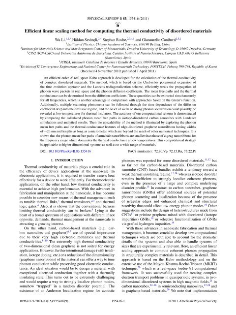
PHYSICAL REVIEW B 83, 155416 (2011)
Efficient linear scaling method for computing the thermal conductivity of disordered materials
Wu Li, 1,2,* Hâldun Sevinçli, 2,* Stephan Roche, 2,3,4,† and Gianaurelio Cuniberti2,5,‡ 1Institute of Physics, Chinese Academy of Sciences, 100190 Beijing, China
2Institute for Materials Science and Max Bergmann Center of Biomaterials, Dresden University of Technology, D-01062 Dresden, Germany
3CIN2 (ICN-CSIC) and Universitat Autónoma de Barcelona, Catalan Institute of Nanotechnology, Campus UAB, 08193 Bellaterra
(Barcelona), Spain
4ICREA, Institució Catalana de Recerca i Estudis Avancats, 08070 Barcelona, Spain
5Division of IT Convergence Engineering and National Center for Nanomaterials Technology, POSTECH, Pohang 790-784, Republic of Korea
(Received 4 November 2010; published 7 April 2011)
An efficient order-N real-space Kubo approach is developed for the calculation of the thermal conductivity
of complex disordered materials. The method, which is based on the Chebyshev polynomial expansion of
the time evolution operator and the Lanczos tridiagonalization scheme, efficiently treats the propagation of
phonon wave packets in real space and the phonon diffusion coefficients. The mean free paths and the thermal
conductance can be determined from the diffusion coefficients. These quantities can be extracted simultaneously
for all frequencies, which is another advantage in comparison with approaches based on the Green’s function.
Additionally, multiple scattering phenomena can be followed through the time dependence of the diffusion
coefficient deep into the diffusive regime, and the onset of weak or strong phonon localization could possibly be
revealed at low temperatures for thermal insulators. The accuracy of our computational scheme is demonstrated
by comparing the calculated phonon mean free paths in isotope-disordered carbon nanotubes with Landauer
simulations and analytical results. Then the upscalability of the method is illustrated by exploring the phonon
mean free paths and the thermal conductance features of edge-disordered graphene nanoribbons having widths
of ∼20 nm and lengths as long as a micrometer, which are beyond the reach of other numerical techniques. It is
shown that the phonon mean free paths of armchair nanoribbons are smaller than those of zigzag nanoribbons for
the frequency range which dominates the thermal conductance at low temperatures. This computational strategy
is applicable to higher-dimensional systems as well as to a wide range of materials.
DOI: 10.1103/PhysRevB.83.155416 PACS number(s): 72.80.Vp, 72.15.Rn, 73.22.Pr
I. INTRODUCTION
Thermal conductivity of materials plays a crucial role in
the efficiency of device applications at the nanoscale. In
electronic applications, it is required to transfer excess heat
effectively for a device to work efficiently. For thermoelectric
applications, on the other hand, low thermal conductivity is
essential to achieve high performance. With the advances in
fabrication and manipulation at the nanoscale, it has become
possible to consider new means of thermal management such
as tunable thermal links, 1 thermal transistors, 2,3 and thermal
logic gates. 4 Also, it is shown that the conventional barriers
limiting thermal conductivity can be broken. 5 Lying at the
heart of a broad spectrum of applications with different, if not
opposite, demands, thermal management at the nanoscale is
attracting a growing interest.
On the other hand, carbon-based materials (e.g., carbon
nanotubes and graphene) 6,7 are of special importance
due to their very high electronic mobilities and thermal
conductivities. 8–10 The extremely high thermal conductivity
of two-dimensional clean graphene is not suited for energy
applications. However, further intentional damage (with irradiation,
isotope doping, etc.) or a reduction of the dimensionality
(graphene nanoribbons) of the material can offer a way to tune
phonon conduction while preserving good electronic conductance.
An ideal situation would be to design a material with
exceptional electrical conduction together with a thermally
insulating state. This turns out to be extremely challenging
and would require a way to strongly localize phonon modes,
somehow “trapped” in a random disorder potential. The
existence of an Anderson localization regime for acoustic
phonons was reported for some disordered materials, 11,12 but
so far not for carbon-based materials. Disordered carbon
nanotube (CNT)-based bundles exhibit a tendency toward a
weak thermal insulating regime, 13,14 whereas isotope disorder
remains inefficient to strongly localize coherent phonons,
even in the presence of a large and complex underlying
disorder profile. 15 In contrast to carbon nanotubes, graphene
nanoribbons (GNRs) offer additional sources of potential
phonon scattering and localization because of the presence
of irregular edges and enhanced chemical and structural
reactivity that could affect low-energy phonon modes. 16 Other
suggestions include the design of heterostructures made from
CNTs 17 or pristine graphene mixed with disordered (isotope
impurities) GNRs, 18 or selective functionalization of GNRs
via grafted hydrogen impurities. 19
With these advances in nanoscale fabrication and thermal
management, it becomes crucial to develop new computational
techniques which are both able to account for the atomistic
details of the systems and also able to handle systems of
sizes that are experimentally relevant. Here, an efficient linear
scaling approach to compute coherent phonon propagation
in structurally complex materials is described in detail. This
approach is based on the Kubo methodology and on the
extensive use of the Mayou-Khanna-Roche-Triozon (MKRT)
technique, 20 which is a real-space (order-N) computational
framework. It was successfully used for treating complex
electron transport problems in quasiperiodic systems, in twodimensional
disordered systems in high magnetic fields, 21 in
carbon nanotubes, 22–26 in semiconducting nanowires, 27,28 and
in graphene-based materials. 29 We note that implementation
1098-0121/2011/83(15)/155416(9) 155416-1
©2011 American Physical Society

LI, SEVINÇLI, ROCHE, AND CUNIBERTI PHYSICAL REVIEW B 83, 155416 (2011)
of the Lanczos method for computing the Landauer-Büttiker
conductance of low-dimensional systems was also reported. 30
In this paper, we first extend our recent communication
on the method 31 to a complete derivation of the phonon
transmission coefficient starting from the original Kubo
formula and within the harmonic approximation. This means
that only elastic scattering (due, for instance, to isotope
disorder) is introduced, disregarding anharmonic effects. The
study of the dynamical properties of phonon wave packets
is also related to the thermal conductance, which requires a
phonon frequency integration over the whole spectrum. We
then validate the method by comparison with other numerical
approaches and analytical results, and we further apply this
method to edge-disordered GNRs and discuss its limits.
II. COMPUTATIONAL PHONON TRANSPORT
METHODOLOGY
The electronic transport theory in the linear response regime
generally relies on the approach derived by Kubo. 32 To investigate
bulk quantum phonon transport in disordered materials,
the use of the Kubo formalism turns out to be the most natural
and computationally efficient one. It has already been used for
investigating thermal transport in disordered binary alloys or
nanocrystalline silicon. 33,34 Inspired by the MKRT scheme for
electron transport, 20 we derive a real-space implementation of
the Kubo formula for phonon propagation, which establishes
a direct computational bridge between phonon dynamics and
thermal conductance. In contrast to other implementations of
the Kubo approach, we extract dynamical information from the
time evolution of the wave packet 35 (based on the expansion of
the evolution operator on a Chebyshev polynomials basis) and
simulate quantum dynamics instead of solving the Newtonian
equations of motion. 36–38 Therefore, a single initial condition is
enough (i.e., the initial atomic displacements) without any need
to compute the time-dependent atomic velocities. Additionally,
by using the Lanczos technique, one can avoid any matrix
inversions, and a considerable gain in computational efficiency
is obtained, which allows the study of very large-scale
materials.
A. Derivation of the phonon transport equations
The vibrational Hamiltonian, taking only the harmonic
interactions into account, is described as
H = ˆp
i
2 i
+
2Mi
ij ûiûj , (1)
ij
where ûi and ˆpi are the displacement and momentum operators
for the ith atomic degree of freedom, Mi is the corresponding
mass, and is the force constant tensor. Based on the
linear response theory, the phonon conductivity σ along the x
direction can be obtained as34 σ = T −1 β ∞
lim lim dλ dt e
ω→0 η→0 0 0
i(ω+iη)t 〈 Jˆ x (−i¯hλ) Jˆ x (t)〉,
(2)
with being the system volume and T being the temperature;
Jˆ x is the x component of the energy flux operator ˆJ, and it can
be expressed as Jˆ x = 1/2
ij (Xi − Xj )ij ûi ˆvj , where ˆvj
is the velocity operator and Xi is the equilibrium position of
the atom to which the ith degree of freedom belongs. After
neglecting terms like â † mâ † n and âmân, Jˆ x can be rewritten in
terms of the phonon creation and annihilation operators as
Jˆ x =
m,n J x mn↠mân, where
J x mn =−i¯h
ωm ωn
+ 〈m|[X,D]|n〉. (3)
4 ωn ωm
In Eq. (3), X is the diagonal matrix of equilibrium positions,
D is the mass normalized dynamical matrix with Dij =
ij / MiMj , and |n〉 is the nth eigenstate of D. Allen and
Feldman have shown that Eq. (2) can be written as34 σ = π ∂fB
J
¯hT ∂ωm m,n
x mnJ x nmδ(ωm − ωn), (4)
where fB is the Bose distribution function. Therefore, one has
σ =− π
∞
dω
0
¯h ∂fB
4ω ∂T
× Tr{[ ˆX,D]δ(ω − √ D)[ ˆX,D]δ(ω − √ D)}, (5)
where √ D =
n ωn|n〉〈n| acts as the free particle Hamiltonian,
δ(···) is the Dirac delta function, and Tr{···}stands for
the trace operator. Defining Vx =−i[X, √ D], one can write
the thermal conductance of a one-dimensional system as
κ = π
L2 ∞
dω¯hω
0
∂fB
∂T Tr{Vxδ(ω − √ D)Vxδ(ω − √ D)}.
(6)
The thermal conductance can also be derived from the
Landauer formalism39 or the nonequilibrium Green’s function
approach40 as
κ = 1
∞
dω¯hω
2π 0
∂fB
T (ω), (7)
∂T
with T (ω) being the phonon transmission function. Comparing
these two formulas, we obtain the transmission function as
155416-2
2 2π
T (ω) =
L2 Tr{Vxδ(ω − √ D)Vxδ(ω − √ D)}. (8)
The phonon transmission function derived here has exactly the
same form as the electron transmission function derived from
the Kubo-Greenwood formula, 20
Tel(E) = 2π 2¯h 2
L2 Tr{ ˆVxδ(E − ˆHel) ˆVxδ(E − ˆHel)}, (9)
where ˆHel is the electronic Hamiltonian.
We rewrite the Kubo formula in a more convenient form for
the real-space study of the wave-packet dynamics. Expressing
the δ-function as
δ(ω − √ D) = 1
∞
dt e
2π −∞
i(ω−√D)t , (10)
one can then rewrite T (ω)L2 /π as
∞
dtTr{δ(ω − √ D)}〈Vx(t)Vx(0)〉ω
−∞
∞
=
0
dtTr{δ(ω − √ D)}〈Vx(t)Vx(0) + Vx(0)Vx(t)〉ω,
(11)

EFFICIENT LINEAR SCALING METHOD FOR COMPUTING ... PHYSICAL REVIEW B 83, 155416 (2011)
where Vx(t) = U † (t)VxU(t) with U(t) = e −i√ Dt , and 〈···〉ω
denotes the mean value of the operator over different eigenstates
with frequency ω. The mean-square displacement along
the x direction over the states having frequency ω is written as
χ 2 (ω,t) =〈(X(t) − X(0)) 2 〉ω, (12)
where χ(t) = U † (t)χU(t). Hence,
d
dt χ 2 (ω 2 ,t) =〈Vx(0)(X(0) − X(−t))
+ (X(0) − X(−t))Vx(0)〉ω, (13)
and
d2 dt2 χ 2 (ω 2 ,t) =〈Vx(t)Vx(0) + Vx(0)Vx(t)〉ω. (14)
Using d
dt χ 2 (ω2 ,t)|t=0 = 0, the integral in Eq. (11) can be
evaluated as
T (ω) = 2ωπ
L2 Tr{δ(ω2 d
− D)} lim
t→∞ dt χ 2 (ω,t). (15)
We consider 〈Vx(0)Vx(t)〉ω = v2 (ω)e−t/τtr , where v(ω) and τtr
stand for the average group velocity and the average transport
time at frequency ω, respectively. With this approximation, the
multiple scattering effects are taken into account in an average
manner, and the mean-square displacement is obtained as
χ 2 (ω,t) = 2v 2 τtrt − 2v 2 τ 2
tr + 2v2τ 2
tre−t/τtr . (16)
The diffusion coefficient is defined as
D(ω,t) = χ 2 (ω,t)
; (17)
t
therefore. in the ballistic regime t ≪ τtr and D(ω,t) = v2t, while in the diffusive regime t ≫ τtr and D(ω,t) = Dmax(ω) =
2v2τtr. The transmission function in the diffusive regime
reduces to
T (ω) = 2ωπ
L2 Tr{δ(ω2 − D)}Dmax(ω). (18)
The phonon transport mean free path (MFP) can be obtained
via
ℓ(ω) = vτtr = Dmax(ω)
. (19)
2v(ω)
We note that ℓ(ω) can also be approximated by T (ω)L/2Nch,
which gives the same result as Eq. (19), because in a quasione-dimensional
system the number of channels is Nch(ω) ≈
2ωπTr{δ(ω2 − D)}v(ω)/L.
By computing D(ω,t), one can thus deduce Dmax(ω) and
v(ω) and ℓ(ω). Noticing that
χ 2 (ω,t) = Tr{(X(t) − X(0))2δ(ω2 − D)}
Tr{δ(ω2 − D)}
= Tr{[X,U(t)]† δ(ω2 − D)[X,U(t)]}
Tr{δ(ω2 , (20)
− D)}
the trace in the numerator can be calculated efficiently
through an average over a few random phase states as
N〈ψ|[X,U(t)] † δ(ω2 − D)[X,U(t)]|ψ〉, where N is the number
of degrees of freedom and the bra-ket corresponds to a
kind of projected density of states (PDOS) associated with the
155416-3
vector [X,U(t)]|ψ〉. PDOS differs from the normal PDOS by
a factor of 1/2ω and is obtained by using the Lanczos method.
The value of Tr{δ(ω2 − D)} is also calculated by averaging
the PDOS of |ψ〉 through the Lanczos method. The vector
[X,U(t)]|ψ〉 is calculated by using the Chebyshev expansion
of U(t); however, the very low frequency component cannot
be evaluated with a reasonable accuracy for large t, which
is discussed in Sec. II C. If we transform U(t) → U(τ) =
e−iDτ , the corresponding velocity and the transport time are
transformed as v → 2ωv and τtr → τtr/2ω, up to the first-order
approximation of the perturbation of the dynamical matrix D.
Therefore, Eq. (20) can be approximated by
χ 2 (ω,t) ≈ Tr{[X,U(t/2ω)]† δ(ω2 − D)[X,U(t/2ω)]}
Tr{δ(ω2 , (21)
− D)}
so we can expand U(τ) instead of U(t) in terms of the
Chebyshev polynomials.
B. Lanczos and continued fraction methods
Efficient computational recursion and order-N methods
have been successfully developed in solid-state physics,
starting from the pioneering work by Haydock. 41–43 The
recursion methods are based on an eigenvalue approach of
Lanczos44 and rely on the computation of Green’s function
matrix elements by continued fraction expansion, which
can be implemented in either real or reciprocal spaces.
These techniques are particularly well suited for treating
disordered materials (e.g., alloys) and defect-related problems,
and they were successfully implemented to tackle impuritylevel
calculations in semiconductors using the tight-binding
approximation, 45 or to investigate the electronic structure of
amorphous semiconductors, transition metals, and metallic
glasses based on linear-muffin-tin orbitals. 46 The vibrational
density of states (DOS) of disordered materials has also been
investigated by the recursion method. 47
Owing to the δ function, the numerator and the denominator
can be considered PDOS on |ψ〉 and [X,U(t)]|ψ〉, respectively.
Given |ψ〉 and assuming that [X,U(t)]|ψ〉 is already known,
we can use the continued fraction method to calculate PDOS.
We tridiagonalize the dynamical matrix D from an initial
state |ψ〉 or [X,U(t)]|ψ〉 by using the Lanczos scheme. The
Lanczos coefficients an and bn display a convenient feature:
they converge rapidly to constants a∞ and b∞, respectively,
for a reasonable number of recursion steps. The PDOS is then
deduced from the first diagonal element of retarded Green’s
function in the tridiagonalized representation. For instance,
〈ψ|δ(ω 2 − D)|ψ〉 =− 1
π lim
η→0 Im〈ψ|
1
ω2 |ψ〉, (22)
+ iη − D
and limη→0〈ψ|(ω 2 + iη − D) −1 |ψ〉 can be expressed as a
continued fraction:
1
ω2 b
+ iη − a1 −
2 1
ω 2 b
+ iη − a2 −
2 .
2
. ..
ω 2 + iη − aN − b 2 N(ω) (23)

LI, SEVINÇLI, ROCHE, AND CUNIBERTI PHYSICAL REVIEW B 83, 155416 (2011)
PDOS (arbitrary unit)
a n
b n
0 20 40 60 80 100
Recursion number n
0 200 400 600 800 1000 1200 1400 1600
ω (cm −1 )
FIG. 1. (Color online) Vibrational PDOS on a single random
phase state for a clean two-dimensional graphene system calculated
by using the force constants given in Ref. 53. The Lanczos coefficients
are shown in the inset.
In practice, the continued fraction is terminated after a certain
step N by the approximation aN+1 = a∞ and bN+1 = b∞.The
termination can be analytically obtained as
(ω) = ω2 + iη − a∞ − i (2b∞) 2 − (ω2 + iη − a∞) 2
.
2b 2 ∞
(24)
As an example, the normal PDOS on a single random phase
state for a clean two-dimensional graphene system is given in
Fig. 1. It already agrees well with the DOS obtained by direct
matrix diagonalization. The inset shows the corresponding
Lanczos coefficients, a(n) and b(n).
C. Chebyshev polynomial expansion
The evolution of the vector [X,U(t)]|ψ〉 is determined by
U(t). Although U(t) has a simple form, its exact calculation
requires diagonalization of the dynamical matrix. Provided
that all the eigenvalues and eigenvectors of D are known,
the matrix form of U(t) can be obtained by using a unitary
transformation. The diagonalization of a matrix requires
O(N 3 ) operations, so it is practically impossible to handle a
system with size N 10 6 . One can employ Taylor expansion,
but the efficiency and the accuracy are difficult to fulfill at
the same time with such an expansion, especially because
higher accuracy requires either a larger number of time steps or
larger expansion orders for a given time t. The implementation
of the Taylor expansion for studying long time propagation
of wave packets in large-scale disordered systems with high
accuracy is therefore beyond today’s computational reach.
Instead, we use orthogonal polynomials. In principle, any set of
orthogonal polynomials could be used for expanding the time
evolution operator. On the other hand, Chebyshev polynomials
have been widely used in past literature due to a particularly
well achieved numerical stability, 20,38 and for this reason
we employ the Chebyshev polynomial expansion approach.
Formally, one can expand any function of an operator in
terms of Chebyshev polynomial-based operators, since the set
of Chebyshev polynomials Qn form a complete orthogonal
basis set. The expansion coefficients depend on the form
of the expanded function, on the time step t, and on the
function domain [a − 2b,a + 2b], which should cover the
whole spectrum of the dynamical matrix D. Since Chebyshev
polynomials are defined in the interval [−1,1], we first need
to scale and shift the argument so that it falls within the range
based on D ′ = (D − a)/2b. Finally, U(t) can be expanded
as
where
cn(t) =
U(t) = e −it√ a+2bD ′
1 2
π(1 + δn,0) −1
=
∞
cn(t)Qn(D ′ ), (25)
n=0
dx ′ 1
√
1 − x ′2 e−it√ a+2bx ′
Qn(x ′ ).
(26)
Thus, [X,U(t)]|ψ〉 = ∞
n=0 cn(t)[X,Qn(D)]|ψ〉. Then
the commutators are computed using the Chebyshev recurrence
relation bQn+1(D ′ ) = (D − a)Qn(D ′ ) − bQn−1(D ′ ),
where Q0(D ′ ) = 1 and Q1(D ′ ) = (D − a)/2b. Recurrence
relations between commutators write b[X,Qn+1(D ′ )] =
[X,(D − a)Qn(D ′ )] − b[X,Qn−1(D ′ )], which is rewritten for
convenience as
|αn〉 =Qn(D ′ )|ψ〉, |βn〉 =[X,Qn(D ′ )]|ψ〉. (27)
Using the well-known expression [A,BC] = [A,B]C +
B[A,C], the commutator relationship becomes b|βn+1〉 =
(D − a)|βn〉−b|βn−1〉+[X,D]|αn〉 with |β0〉 =0 and
|β1〉 =[X,D]|ψ〉/2b. The computation of |βn〉 requires the
knowledge of vectors |αn〉 =Qn(D ′ )|ψ〉 that appear in the
Chebyshev expansion of the evolution operator U(T )|ψ〉.
Such |αn〉 vectors satisfy
b|αn+1〉 =(D − a)|αn〉−b|αn−1〉, (28)
with |α0〉 =|ψ〉 and |α1〉 =(D − a)|ψ〉/2b. The algorithm
thus consists of computing in parallel two recurrence relations
and summing up the series:
and
Npoly
U(t)|ψ〉 = cn(t)|αn〉 (29)
n=0
Npoly
[X,U(t)]|ψ〉 = cn(t)|βn〉. (30)
n=0
To reach the desired accuracy, the number of recursion steps
(Npoly) needs to be chosen appropriately depending on the
evolution step and the spectral bandwidth. Once U(mt)|ψ〉
and [X,U(mt)]|ψ〉 are obtained at time mt, then for the
following evolution step one has
and
155416-4
U((m + 1)t)|ψ〉 =[X,U(t)]U(mt)]|ψ〉 (31)
[X,U((m + 1)t)]|ψ〉 =[X,U(t)]U(mt)|ψ〉
+ U(t)[X,U(mt)]|ψ〉. (32)

EFFICIENT LINEAR SCALING METHOD FOR COMPUTING ... PHYSICAL REVIEW B 83, 155416 (2011)
Error
10 −2
10 −4
10 −6
10 0
10 −2
10 −4
Real part
Imaginary part
10
0 30 60 90 120
−6
n
0 1000 2000 3000 4000 5000
x
FIG. 2. (Color online) Error in the modulus of the Chebyshev
approximation for f (x) = e −i√ x with x ∈ [0,10 4 ], a = 5000, b =
2500, and Npoly = 200. In the inset, the absolute value of the real parts
and the imaginary parts of the corresponding Chebyshev coefficients
are shown, respectively.
Thus, the evolution of [X,U(t)]|ψ〉 can be calculated step
by step from any starting |ψ〉 provided cn in Eq. (26) are
known. Accordingly, the algorithm scales linearly with the
system size and the computation time.
For U(t) = e−i√Dt , these coefficients cannot be calculated
explicitly. We therefore have to introduce a discrete grid and
employ a numerical quadrature formula. Here we use the
Chebyshev-Gauss grid of which the interpolating points are
the N zeros of QN(x ′ ):
x ′
1
π k + 2
k = cos
, k = 0,1,...,N− 1, (33)
N
and the related quadrature formula is
1
−1
dx ′ f (x′ N−1
) π
√ = f (x
1 − x ′2 N
′ k ). (34)
The calculated expansion coefficients are plotted in the inset
of Fig. 2 for f (x) = e−i√x 4 with x ∈ [0,10 ], a = 5000, and
b = 2500. After some steps, cn is seen to decay toward zero.
The decay rate of the imaginary part is much slower than the
real part, due to the fact that the imaginary part of e−i√x is not
differentiable at zero. The error of the approximated modulus
with Npoly = 200 is shown in Fig. 2. The approximation
maintains good accuracy when x is not close or equal to
zero. However, the error around x = 0 is very large, which
indicates the time evolution based on the expansion of
U(t) is unstable. If we transform U(t) → U(τ) = e−iDτ ,the
Chebyshev expansion coefficients in Eq. (25) can be evaluated
analytically,
1
k=0
2
cn(τ) =
π(1 + δn,0)
dx
−1
′ 1
√
1 − x ′2 e−iτ(a+2bx′ )
Qn(x ′ )
2
= e
1 + δn,0
−iaτ (−i) n Jn(2bτ), (35)
of which both the real part and the imaginary parts decay
rapidly with n, resulting in high accuracy of the truncation
approximation for the whole spectrum.
III. RESULTS AND DISCUSSION
A. Isotope-disordered CNT
An interesting source of phonon scattering is the isotope
disorder. In carbon-based materials (e.g., nanotubes and
graphene), the controlled incorporation of 13C impurities has
been experimentally demonstrated. 48,49 The question about a
possible coherent localization phenomenon in such disordered
nanostructures was discussed in Ref. 15 using the Green’s
function method. As a test case, we investigate a CNT(7,0) with
10.7% 14C impurities to validate our numerics in comparison
with the Green’s function results15 and also with the analytical
formula for the elastic MFP,
ℓe(ω) =
12aNucNch(ω)
π 2f
M
M
2 ρ2 , (36)
uc (ω)ω2
where a is the length of the lattice vector in the translational
direction, Nuc is the number of atoms in each unit cell, ρuc is the
density of states per unit cell, f is the percentage of isotopic
impurities having mass difference M, and M is the average
mass of the atoms (see Refs. 36 and 50). Figure 3 displays the
evolution of the wave-packet dynamics for phonon modes with
different frequencies. The linear increase of D(ω,t) att>0
observed in all cases indicates ballistic transport at relatively
short distances, whereas the decrease of D(ω,t) for the mode
with frequency ω = 900 cm −1 at t 50 ps is a signature
of localization phenomena. The saturation of D(ω,t) toa
maximum value characterizes diffusive transport. From the
saturation values, the evolution of the elastic MFP (ℓe 2ℓ)
as a function of the phonon frequency and disorder features
can be extracted. The results compare well with those obtained
with Green functions 15 (Fig. 4), as well as with Eq. (36)
(Fig. 4, inset). Only at singularities of the phonon spectrum,
where disorder induces a broadening of states which affect the
Diffusion Coefficient (nm 2 /ps)
155416-5
2500
2000
1500
1000
500
ω=300cm −1
ω=600cm −1
ω=900cm −1
0
0 50 100
Time (ps)
150 200
FIG. 3. (Color online) Time-dependent diffusion coefficients
D(ω,t) for the system of CNT with 10.7% 14 C isotope disorder at
three chosen frequencies.

LI, SEVINÇLI, ROCHE, AND CUNIBERTI PHYSICAL REVIEW B 83, 155416 (2011)
FIG. 4. (Color online) Frequency-dependent elastic MFP (ℓe)
in CNT with isotopic disorder (10%) obtained by using the Kubo
method, the Green’s function method (data taken from Ref. 15 by
courtesy), and the analytical formula.
numerical MFP, do they differ more from those obtained with
the analytical expression.
B. Edge-disordered graphene nanoribbons
GNRs are strips of graphene with widths varying from
a few to several tens of nanometers, depending on their
fabrication processes. 7 In contrast to the two-dimensional
graphene, which is a zero-gap semiconductor, the narrow
lateral size of GNRs entails quantum confinement effects
and allows a modulation of the corresponding electronic band
gap. The vibrational band structures are also affected by the
confinement. 51 Two types of GNRs with highly symmetric
edge shapes, i.e., zigzag GNRs (ZGNRs) and armchair GNRs
(AGNRs), have been predicted and experimentally observed
(see Ref. 7 for a review). Here we consider ZGNRs of different
widths with edge disorder and evaluate the corresponding
transport MFPs. The comparison of the transport MFPs and
the thermal conductances of ZGNR with AGNR having the
same width is also studied.
We use the fourth-nearest-neighbor force constants for
building the dynamical matrices. 52,53 The ribbon widths are
defined with the number of zigzag chains Nz = 20, 40, and 80
for ZGNR, and the number of dimers Na = 138 for AGNR.
The relative amount of edge defects (removed carbon atoms at
the edges) is chosen to be 10%.
Figure 5 (top) shows the frequency-dependent behavior
ℓ(ω) of the zigzag ribbon with Nz = 80 for 10% edge disorder.
Large modulations of ℓ(ω) driven by the underlying vibrational
band structure are observed. For a fixed disorder strength,
the MFP is found to increase almost linearly with the ribbon
width. In Fig. 5 (bottom), the ratio ℓNz /ℓNz is plotted for
1 2
Nz = 20, 40, and 80, keeping the width ratio the same.
One observes that the scaling ℓNz=80/ℓNz=40 ℓNz=40/ℓNz=20
generally holds. This behavior is due to the fact that the
scattering rate decreases with increasing width, a behavior
previously reported for electron transport in both disordered
CNTs and GNRs. 54 Since the minimum accessible frequency
within a reasonable computation time is limited, Dmax could
not be reached for ω

EFFICIENT LINEAR SCALING METHOD FOR COMPUTING ... PHYSICAL REVIEW B 83, 155416 (2011)
κ (nW/K)
40
35
30
25
20
15
10
5
pristine
L=100 nm
L=500 nm
L=1 μm
L=2 μm
0
0 100 200 300 400 500
Temperature (K)
FIG. 7. (Color online) Thermal conductance for the ZGNR (Nz =
80, solid lines) and the AGNR (Na = 138, dashed lines) with edge
disorder of 10% and various ribbon lengths.
thermal conductance of AGNRs to be smaller than that of the
ZGNRs for a fixed-edge disorder strength and ribbon length.
Although the difference is found to be reduced as the ribbon
width increases (not shown), coherent phonon propagation is
still sensitive to the ribbon edge shape.
C. Limits of the methodology
The fact that the relaxation time and the mean free path
diverge as ω → 0 introduces a physical limit to calculate the
mean free paths using real-time simulation techniques. Therefore,
there always exists a nonzero frequency, below which
the diffusion coefficient D(t) does not reach its maximum
value within a given computation time, and this sets a lowest
accessible frequency ωmin. The phonon wave-packet dynamics
is originally determined by the time evolution operator U(t);
however, the Chebyshev expansion of U(t) has a relatively
large error for low frequencies (see Fig. 2). Therefore, it is
preferable to use U(t) in place of U(t) for the sake of accuracy.
However, the evolution of low-frequency modes is slower
with U(t), and ωmin increases within a given computation
time, which creates a computational limit. The accuracy of
the results with U(t) needs to be checked when the disorder
in the system is relatively strong. In the case of very strong
disorder, the approximation is less accurate, and one has to
use the expansion of U(t) directly. Even though the time
evolution based on the expansion of U(t) cannot give the
correct information about very low frequency modes, features
for the high-frequency modes can still be extracted, provided
that the time step and the number of Chebyshev polynomials
are chosen properly. The lowest accessible frequency by using
* The first two authors contributed equally and share the first
authorship of this work.
† stephan.roche@icn.cat
‡ g.cuniberti@tu-dresden.de
1 C. W. Chang, D. Okawa, H. Garcia, T. D. Yuzvinsky, A. Majumdar,
and A. Zettl, Appl. Phys. Lett. 90, 193114 (2007).
155416-7
U(t) can be smaller than the one from U(τ), depending on the
system. We also note that ωmin depends on the computational
capability. Since one can upscale the calculations by means
of high-performance computing, materials other than carbon
are within reach of the presented scheme. It is also worth
mentioning that, even without high-performance computation
techniques, we could achieve mean free paths as long as a few
micrometers, at the same order of magnitude with experimental
sample sizes. At these length scales, boundary scattering is the
detrimental scattering mechanism.
For systems where anharmonicity plays an important role,
an extension of the current methodology is required to account
for dissipation effects and phonon lifetimes. The inclusion
of anharmonic effects is beyond the scope of this study and
deserves further consideration.
IV. CONCLUSION
We have presented an efficient linear scaling approach to
compute coherent phonon wave-packet propagation in real
space and to evaluate the related thermal conductance. The
computational accuracy and efficiency were demonstrated for
isotope disordered carbon nanotubes and large-width graphene
nanoribbons with edge disorder, respectively. A strong impact
of edge-disorder profile on the thermal conductance was found,
as well as an edge shape dependence of thermal conductance,
opening interesting perspectives for thermoelectrical applications.
One should remark that this linear scaling method can
be implemented without major difficulty for a wide range of
other materials, including boron-nitride-based materials 55 or
silicon-based materials (nanowires, superlattices, etc.). 56
ACKNOWLEDGMENTS
This work was supported by the priority program Nanostructured
Thermoelectrics (SPP-1386) of the German Research
Foundation (DFG Contract No. CU 44/11-1), the cluster
of excellence of the Free State of Saxony ECEMP—European
Center for Emerging Materials and Processes Dresden (Project
No. A2), the European Social Funds in Saxony (research group
InnovaSens), and the Alexander von Humboldt Foundation.
This work is also supported by the NANOSIM-GRAPHENE
Project No. ANR-09-NANO-016-01 funded by the French
National Agency (ANR) in the frame of its 2009 program
in Nanosciences, Nanotechnologies and Nanosystems
(P3N2009) and by the World Class University program sponsored
by the South Korean Ministry of Education, Science, and
Technology Program, Project No. R31-2008-000-10100-0.
The authors are thankful to N. Mingo for fruitful discussions.
W.L. thanks the CAS-MPG joint doctoral promotion program.
The Center for Information Services and High Performance
Computing (ZIH) at TU-Dresden is acknowledged.
2B. Li, L. Wang, and G. Casati, Appl. Phys. Lett. 88, 143501
(2006).
3L.-A. Wu and D. Segal, Phys. Rev. Lett. 102, 095503 (2009).
4L. Wang and B. Li, Phys.Rev.Lett.99, 177208 (2007).
5G. Pernot, M. Stoffel, I. Savic, F. Pezzoli, P. Chen, G. Savelli,
A. Jacquot, J. Schumann, U. Denker, I. Mönch, Ch. Deneke, O. G.

LI, SEVINÇLI, ROCHE, AND CUNIBERTI PHYSICAL REVIEW B 83, 155416 (2011)
Schmidt, J. M. Rampnoux, S. Wang, M. Plissonnier, A. Rastelli,
S. Dilhaire, and N. Mingo, Nat. Mater. 9, 491 (2010).
6J. C. Charlier, X. Blase, and S. Roche, Rev. Mod. Phys. 79, 677
(2007).
7A. Cresti, N. Nemec, B. Biel, G. Niebler, F. Triozon, G. Cuniberti,
and S. Roche, Nano Res. 1, 361 (2008).
8A. A. Balandin, S. Ghosh, W. Bao, I. Calizo, D. Teweldebrhan,
F. Miao, and C. N. Lau, Nano Lett. 8, 902 (2008).
9J. H. Seol, I. Jo, A. L. Moore, L. Lindsay, Z. H. Aitken, M. T. Pettes,
X. Li, Z. Yao, R. Huang, D. Broido, N. Mingo, R. S. Ruoff, and
L. Shi, Science 328, 213 (2010).
10E. Pop, Nano Res. 3, 147 (2010); M.-H. Bae, C.-Y. Ong, D. Estrada,
and E. Pop, Nano Lett. 10, 4787 (2010).
11P. W. Anderson, Phys. Rev. 109, 1492 (1958).
12A. Lagendijk, B. van Tiggelen, and D. S. Wiersma, Phys. Today 62,
24 (2009).
13J. Che, T. Ça˘gın, and W. A. Goddard, Nanotechnology 11, 65
(2000).
14R. S. Prasher, X. J. Hu, Y. Chalopin, N. Mingo, K. Lofgreen, S. Volz,
F. Cleri, and P. Keblinski, Phys.Rev.Lett.102, 105901 (2009).
15I. Savic, N. Mingo, and D. A. Stewart, Phys.Rev.Lett.101, 165502
(2008).
16H. Sevinçli and G. Cuniberti, Phys. Rev. B 81, 113401 (2010).
17G. Stoltz, N. Mingo, and F. Mauri, Phys.Rev.B80, 113408 (2009).
18N. Mingo, K. Esfarjani, D. A. Broido, and D. A. Stewart, Phys. Rev.
B 81, 045408 (2010).
19X.Ni,G.Liang,J.-S.Wang,andB.Li,Appl. Phys. Lett. 95, 192114
(2009).
20D. Mayou, Europhys. Lett. 6, 549 (1988); D. Mayou and S. N.
Khanna, J. Phys. I (France) 5, 1199 (1995); S. Roche and D. Mayou,
Phys.Rev.Lett.79, 2518 (1997); F. Triozon, J. Vidal, R. Mosseri,
and D. Mayou, Phys. Rev. B 65, 220202 (2002).
21S. Roche, Phys. Rev. B 59, 2284 (1999); W. Zhu, Q. W. Shi,
X.R.Wang,J.Chen,J.L.Yang,andJ.G.Hou,Phys. Rev. Lett.
102, 056803 (2009).
22S. Roche, J. Jiang, F. Triozon, and R. Saito, Phys.Rev.Lett.95,
076803 (2005).
23H. Ishii, N. Kobayashi, and K. Hirose, Phys. Rev. B 76, 205432
(2007).
24S. Roche and R. Saito, Phys. Rev. Lett. 87, 246803 (2001);
F. Triozon, S. Roche, A. Rubio, and D. Mayou, Phys. Rev. B 69,
121410 (2004); S. Latil, S. Roche, D. Mayou, and J. C. Charlier,
Phys. Rev. Lett. 92, 256805 (2004); S. Latil, F. Triozon, and
S. Roche, ibid. 95, 126802 (2005); Ch. Adessi, S. Roche, and
X. Blase, Phys.Rev.B73, 125414 (2006); R. Avriller, S. Latil,
F. Triozon, X. Blase, and S. Roche, ibid. 74, 121406 (2006).
25S. Roche, J. Jiang, F. Triozon, and R. Saito, Phys.Rev.B72, 113410
(2005).
26H. Ishii, S. Roche, N. Kobayashi, and K. Hirose, Phys. Rev. Lett.
104, 116801 (2010).
27T. Markussen, R. Rurali, M. Brandbyge, and A.-P. Jauho, Phys.
Rev. B 74, 245313 (2006).
28A. Lherbier, M. P. Persson, Y. M. Niquet, F. Triozon, and S. Roche,
Phys. Rev. B 77, 085301 (2008); M. P. Persson, A. Lherbier, Y. M.
Niquet, F. Triozon, and S. Roche, Nano Lett. 8, 4146 (2008).
29A. Lherbier, B. Biel, Y.-M. Niquet, and S. Roche, Phys. Rev.
Lett. 100, 036803 (2008); A. Lherbier, X. Blase, Y.-M. Niquet,
F. Triozon, and S. Roche, ibid. 101, 036808 (2008).
30F. Triozon and S. Roche, Eur. Phys. J. B 46, 427 (2005).
155416-8
31W.Li,H.Sevinçli, G. Cuniberti, and S. Roche, Phys. Rev. B 82,
041410 (2010).
32R. Kubo, J. Phys. Soc. Jpn. 12, 570 (1957); D. Fisher and P. A. Lee,
Phys. Rev. B 23, 6851 (1981).
33A. Alam and A. Mookerjee, Phys. Rev. B 72, 214207 (2005);
A. Bodapati, P. K. Schelling, S. R. Phillpot, and P. Keblinski, ibid.
74, 245207 (2006).
34P. B. Allen and J. L. Feldman, Phys. Rev. Lett. 62, 645 (1989);
Phys. Rev. B 48, 12581 (1993).
35G. G. Naumis, F. Salazar, and C. Wang, Philos. Mag. 86, 1043
(2006); N. Kondo, T. Yamamoto, and K. Watanabe, Jpn. J. Appl.
Phys. 45, L963 (2006); S. Monturet and N. Lorente, Phys. Rev. B
78, 035445 (2008).
36G. P. Srivastava, The Physics of Phonons (Taylor and Francis, New
York, 1990).
37P. K. Schelling, S. R. Phillpot, and P. Keblinski, Phys. Rev. B 65,
144306 (2002).
38Y. L. Loh, S. N. Taraskin, and S. R. Elliott, Phys.Rev.E63, 056706
(2001).
39L. G. C. Rego and G. Kirczenow, Phys. Rev. Lett. 81, 232 (1998);
N. Mingo, Phys. Rev. B 74, 125402 (2006); N. Mingo and L. Yang,
ibid. 68, 245406 (2003).
40A. Özpineci and S. Ciraci, Phys. Rev. B 63, 125415 (2001);
T. Yamamoto and K. Watanabe, Phys. Rev. Lett. 96, 255503 (2006).
41R. Haydock, in Solid State Physics, edited by H. Ehrenreich, F. Seitz
and D. Turnbull (Academic, New York, 1980), Vol. 35, p. 215.
42Recursion Method and Its Applications, edited by D. G. Petitfor
and D. L. Weaire, Springer Series in Solid State Sciences,
Vol. 58 (Springer-Verlag, Berlin, 1985); The Recursion Method:
Application to Many-Body Dynamics, editedbyV.S.Viswanath
and G. Müller, Lecture Notes in Physics, Vol. 23 (Springer-Verlag,
Berlin, 1994).
43T. Hoshi and T. Fujiwara, J. Phys. Soc. Jpn. 72, 2429 (2003);
J. Phys. Condens. Matter 18, 10787 (2006).
44C. Lanczos, J. Res. Natl. Bur. Stand. 45, 255 (1950).
45D. J. Lohrmann, L. Resca, G. P. Parravicini, and R. D. Graft, Phys.
Rev. B 40, 8404 (1989).
46S. K. Bose, K. Winer, and O. K. Andersen, Phys. Rev. B 37, 6262
(1988); S. K. Bose, S. S. Jaswal, O. K. Andersen, and J. Hafner,
ibid. 37, 9955 (1988); S. K. Bose, J. Kudrnovsky, I. I. Mazin, and
O. K. Andersen, ibid. 41, 7988 (1990).
47P. M. Lam, W. Bao, and Z. Zheng, Z. Phys. B 59, 63 (1985).
48V. Zólyomi, F. Simon, A. Rusznyak, R. Pfeiffer,
H. Peterlik, H. Kuzmany, and J. Kurti, Phys. Rev. B 75,
195419 (2007).
49X. Li, W. Cai, L. Colombo, and R. S. Ruoff, Nano Lett. 9, 4268
(2009).
50P. G. Klemens, Proc. R. Soc. A 208, 108 (1951).
51R. Gillen, M. Mohr, J. Maultzsch, and C. Thomsen, Phys. Rev. B
80, 155418 (2009).
52R. Saito, G. Dresselhaus, M. S. Dresselhaus, Physical Properties of
Carbon Nanotubes (Imperial College Press, London, 1998).
53J. Zimmermann, P. Pavone, and G. Cuniberti, Phys. Rev. B 78,
045410 (2008).
54C. T. White and T. N. Todorov, Nature 393, 240 (1998); S. Roche,
G. Dresselhaus, M. S. Dresselhaus, and R. Saito, Phys. Rev. B 62,
16092 (2000); D. A. Areshkin, D. Gunlycke, and C. T. White, Nano
Lett. 7, 204 (2007); A. Cresti and S. Roche, Phys. Rev. B 79, 233404
(2009); New J. Phys. 11, 09500 (2009).

EFFICIENT LINEAR SCALING METHOD FOR COMPUTING ... PHYSICAL REVIEW B 83, 155416 (2011)
55 I. Savic, D. A. Stewart, and N. Mingo, Phys.Rev.B78, 235434
(2008); D. A. Stewart, I. Savic, and N. Mingo, Nano Lett. 9, 81
(2009); L. Ci, L. Song, C. Jin, D. Jariwala, D. Wu, Y. Li, A.
Srivastava, Z. F. Wang, K. Storr, L. Balicas, F. Liu, and P. M.
Ajayan, Nat. Mater. 9, 430 (2010).
155416-9
56 T. Markussen, R. Rurali, A. P. Jauho, and M. Brandbyge, Phys.
Rev. Lett. 99, 076803 (2007); T. Markussen, A.-P. Jauho, and
M. Brandbyge, ibid. 103, 055502 (2009); Phys. Rev. B 79, 035415
(2009); D. Donadio and G. Galli, Phys. Rev. Lett. 102, 195901
(2009).