Efficient linear scaling method for computing the thermal conductivity ...

LI, SEVINÇLI, ROCHE, AND CUNIBERTI PHYSICAL REVIEW B 83, 155416 (2011)
PDOS (arbitrary unit)
a n
b n
0 20 40 60 80 100
Recursion number n
0 200 400 600 800 1000 1200 1400 1600
ω (cm −1 )
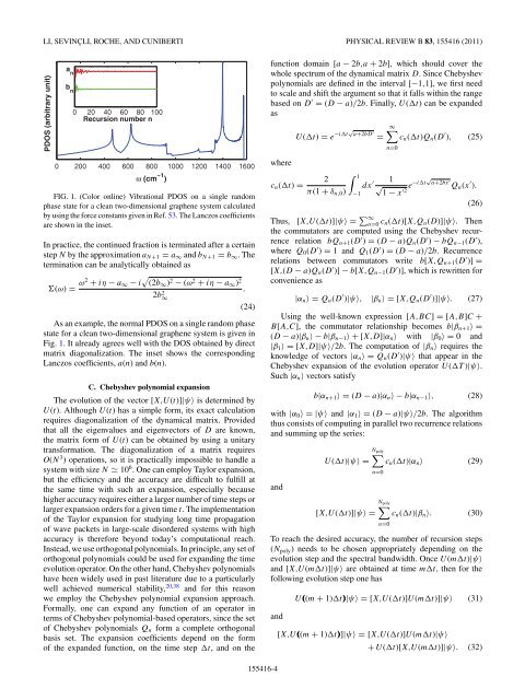
FIG. 1. (Color online) Vibrational PDOS on a single random
phase state for a clean two-dimensional graphene system calculated
by using the force constants given in Ref. 53. The Lanczos coefficients
are shown in the inset.
In practice, the continued fraction is terminated after a certain
step N by the approximation aN+1 = a∞ and bN+1 = b∞.The
termination can be analytically obtained as
(ω) = ω2 + iη − a∞ − i (2b∞) 2 − (ω2 + iη − a∞) 2
.
2b 2 ∞
(24)
As an example, the normal PDOS on a single random phase
state for a clean two-dimensional graphene system is given in
Fig. 1. It already agrees well with the DOS obtained by direct
matrix diagonalization. The inset shows the corresponding
Lanczos coefficients, a(n) and b(n).
C. Chebyshev polynomial expansion
The evolution of the vector [X,U(t)]|ψ〉 is determined by
U(t). Although U(t) has a simple form, its exact calculation
requires diagonalization of the dynamical matrix. Provided
that all the eigenvalues and eigenvectors of D are known,
the matrix form of U(t) can be obtained by using a unitary
transformation. The diagonalization of a matrix requires
O(N 3 ) operations, so it is practically impossible to handle a
system with size N 10 6 . One can employ Taylor expansion,
but the efficiency and the accuracy are difficult to fulfill at
the same time with such an expansion, especially because
higher accuracy requires either a larger number of time steps or
larger expansion orders for a given time t. The implementation
of the Taylor expansion for studying long time propagation
of wave packets in large-scale disordered systems with high
accuracy is therefore beyond today’s computational reach.
Instead, we use orthogonal polynomials. In principle, any set of
orthogonal polynomials could be used for expanding the time
evolution operator. On the other hand, Chebyshev polynomials
have been widely used in past literature due to a particularly
well achieved numerical stability, 20,38 and for this reason
we employ the Chebyshev polynomial expansion approach.
Formally, one can expand any function of an operator in
terms of Chebyshev polynomial-based operators, since the set
of Chebyshev polynomials Qn form a complete orthogonal
basis set. The expansion coefficients depend on the form
of the expanded function, on the time step t, and on the
function domain [a − 2b,a + 2b], which should cover the
whole spectrum of the dynamical matrix D. Since Chebyshev
polynomials are defined in the interval [−1,1], we first need
to scale and shift the argument so that it falls within the range
based on D ′ = (D − a)/2b. Finally, U(t) can be expanded
as
where
cn(t) =
U(t) = e −it√ a+2bD ′
1 2
π(1 + δn,0) −1
=
∞
cn(t)Qn(D ′ ), (25)
n=0
dx ′ 1
√
1 − x ′2 e−it√ a+2bx ′
Qn(x ′ ).
(26)
Thus, [X,U(t)]|ψ〉 = ∞
n=0 cn(t)[X,Qn(D)]|ψ〉. Then
the commutators are computed using the Chebyshev recurrence
relation bQn+1(D ′ ) = (D − a)Qn(D ′ ) − bQn−1(D ′ ),
where Q0(D ′ ) = 1 and Q1(D ′ ) = (D − a)/2b. Recurrence
relations between commutators write b[X,Qn+1(D ′ )] =
[X,(D − a)Qn(D ′ )] − b[X,Qn−1(D ′ )], which is rewritten for
convenience as
|αn〉 =Qn(D ′ )|ψ〉, |βn〉 =[X,Qn(D ′ )]|ψ〉. (27)
Using the well-known expression [A,BC] = [A,B]C +
B[A,C], the commutator relationship becomes b|βn+1〉 =
(D − a)|βn〉−b|βn−1〉+[X,D]|αn〉 with |β0〉 =0 and
|β1〉 =[X,D]|ψ〉/2b. The computation of |βn〉 requires the
knowledge of vectors |αn〉 =Qn(D ′ )|ψ〉 that appear in the
Chebyshev expansion of the evolution operator U(T )|ψ〉.
Such |αn〉 vectors satisfy
b|αn+1〉 =(D − a)|αn〉−b|αn−1〉, (28)
with |α0〉 =|ψ〉 and |α1〉 =(D − a)|ψ〉/2b. The algorithm
thus consists of computing in parallel two recurrence relations
and summing up the series:
and
Npoly
U(t)|ψ〉 = cn(t)|αn〉 (29)
n=0
Npoly
[X,U(t)]|ψ〉 = cn(t)|βn〉. (30)
n=0
To reach the desired accuracy, the number of recursion steps
(Npoly) needs to be chosen appropriately depending on the
evolution step and the spectral bandwidth. Once U(mt)|ψ〉
and [X,U(mt)]|ψ〉 are obtained at time mt, then for the
following evolution step one has
and
155416-4
U((m + 1)t)|ψ〉 =[X,U(t)]U(mt)]|ψ〉 (31)
[X,U((m + 1)t)]|ψ〉 =[X,U(t)]U(mt)|ψ〉
+ U(t)[X,U(mt)]|ψ〉. (32)