Efficient linear scaling method for computing the thermal conductivity ...
Efficient linear scaling method for computing the thermal conductivity ...
Efficient linear scaling method for computing the thermal conductivity ...

You also want an ePaper? Increase the reach of your titles
YUMPU automatically turns print PDFs into web optimized ePapers that Google loves.
EFFICIENT LINEAR SCALING METHOD FOR COMPUTING ... PHYSICAL REVIEW B 83, 155416 (2011)<br />
Error<br />
10 −2<br />
10 −4<br />
10 −6<br />
10 0<br />
10 −2<br />
10 −4<br />
Real part<br />
Imaginary part<br />
10<br />
0 30 60 90 120<br />
−6<br />
n<br />
0 1000 2000 3000 4000 5000<br />
x<br />
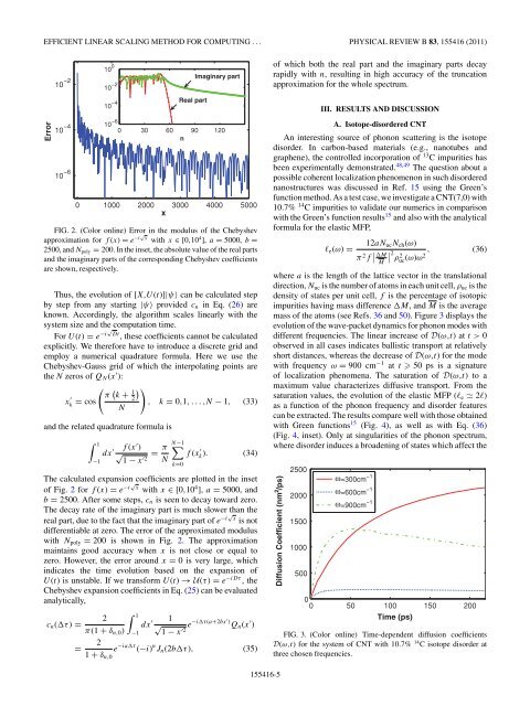
FIG. 2. (Color online) Error in <strong>the</strong> modulus of <strong>the</strong> Chebyshev<br />
approximation <strong>for</strong> f (x) = e −i√ x with x ∈ [0,10 4 ], a = 5000, b =<br />
2500, and Npoly = 200. In <strong>the</strong> inset, <strong>the</strong> absolute value of <strong>the</strong> real parts<br />
and <strong>the</strong> imaginary parts of <strong>the</strong> corresponding Chebyshev coefficients<br />
are shown, respectively.<br />
Thus, <strong>the</strong> evolution of [X,U(t)]|ψ〉 can be calculated step<br />
by step from any starting |ψ〉 provided cn in Eq. (26) are<br />
known. Accordingly, <strong>the</strong> algorithm scales <strong>linear</strong>ly with <strong>the</strong><br />
system size and <strong>the</strong> computation time.<br />
For U(t) = e−i√Dt , <strong>the</strong>se coefficients cannot be calculated<br />
explicitly. We <strong>the</strong>re<strong>for</strong>e have to introduce a discrete grid and<br />
employ a numerical quadrature <strong>for</strong>mula. Here we use <strong>the</strong><br />
Chebyshev-Gauss grid of which <strong>the</strong> interpolating points are<br />
<strong>the</strong> N zeros of QN(x ′ ):<br />
x ′ <br />
1<br />
π k + 2<br />
k = cos<br />
, k = 0,1,...,N− 1, (33)<br />
N<br />
and <strong>the</strong> related quadrature <strong>for</strong>mula is<br />
1<br />
−1<br />
dx ′ f (x′ N−1<br />
) π <br />
√ = f (x<br />
1 − x ′2 N<br />
′ k ). (34)<br />
The calculated expansion coefficients are plotted in <strong>the</strong> inset<br />
of Fig. 2 <strong>for</strong> f (x) = e−i√x 4 with x ∈ [0,10 ], a = 5000, and<br />
b = 2500. After some steps, cn is seen to decay toward zero.<br />
The decay rate of <strong>the</strong> imaginary part is much slower than <strong>the</strong><br />
real part, due to <strong>the</strong> fact that <strong>the</strong> imaginary part of e−i√x is not<br />
differentiable at zero. The error of <strong>the</strong> approximated modulus<br />
with Npoly = 200 is shown in Fig. 2. The approximation<br />
maintains good accuracy when x is not close or equal to<br />
zero. However, <strong>the</strong> error around x = 0 is very large, which<br />
indicates <strong>the</strong> time evolution based on <strong>the</strong> expansion of<br />
U(t) is unstable. If we trans<strong>for</strong>m U(t) → U(τ) = e−iDτ ,<strong>the</strong><br />
Chebyshev expansion coefficients in Eq. (25) can be evaluated<br />
analytically,<br />
1<br />
k=0<br />
2<br />
cn(τ) =<br />
π(1 + δn,0)<br />
dx<br />
−1<br />
′ 1<br />
√<br />
1 − x ′2 e−iτ(a+2bx′ )<br />
Qn(x ′ )<br />
2<br />
= e<br />
1 + δn,0<br />
−iaτ (−i) n Jn(2bτ), (35)<br />
of which both <strong>the</strong> real part and <strong>the</strong> imaginary parts decay<br />
rapidly with n, resulting in high accuracy of <strong>the</strong> truncation<br />
approximation <strong>for</strong> <strong>the</strong> whole spectrum.<br />
III. RESULTS AND DISCUSSION<br />
A. Isotope-disordered CNT<br />
An interesting source of phonon scattering is <strong>the</strong> isotope<br />
disorder. In carbon-based materials (e.g., nanotubes and<br />
graphene), <strong>the</strong> controlled incorporation of 13C impurities has<br />
been experimentally demonstrated. 48,49 The question about a<br />
possible coherent localization phenomenon in such disordered<br />
nanostructures was discussed in Ref. 15 using <strong>the</strong> Green’s<br />
function <strong>method</strong>. As a test case, we investigate a CNT(7,0) with<br />
10.7% 14C impurities to validate our numerics in comparison<br />
with <strong>the</strong> Green’s function results15 and also with <strong>the</strong> analytical<br />
<strong>for</strong>mula <strong>for</strong> <strong>the</strong> elastic MFP,<br />
ℓe(ω) =<br />
12aNucNch(ω)<br />
π 2f <br />
M <br />
M<br />
2 ρ2 , (36)<br />
uc (ω)ω2<br />
where a is <strong>the</strong> length of <strong>the</strong> lattice vector in <strong>the</strong> translational<br />
direction, Nuc is <strong>the</strong> number of atoms in each unit cell, ρuc is <strong>the</strong><br />
density of states per unit cell, f is <strong>the</strong> percentage of isotopic<br />
impurities having mass difference M, and M is <strong>the</strong> average<br />
mass of <strong>the</strong> atoms (see Refs. 36 and 50). Figure 3 displays <strong>the</strong><br />
evolution of <strong>the</strong> wave-packet dynamics <strong>for</strong> phonon modes with<br />
different frequencies. The <strong>linear</strong> increase of D(ω,t) att>0<br />
observed in all cases indicates ballistic transport at relatively<br />
short distances, whereas <strong>the</strong> decrease of D(ω,t) <strong>for</strong> <strong>the</strong> mode<br />
with frequency ω = 900 cm −1 at t 50 ps is a signature<br />
of localization phenomena. The saturation of D(ω,t) toa<br />
maximum value characterizes diffusive transport. From <strong>the</strong><br />
saturation values, <strong>the</strong> evolution of <strong>the</strong> elastic MFP (ℓe 2ℓ)<br />
as a function of <strong>the</strong> phonon frequency and disorder features<br />
can be extracted. The results compare well with those obtained<br />
with Green functions 15 (Fig. 4), as well as with Eq. (36)<br />
(Fig. 4, inset). Only at singularities of <strong>the</strong> phonon spectrum,<br />
where disorder induces a broadening of states which affect <strong>the</strong><br />
Diffusion Coefficient (nm 2 /ps)<br />
155416-5<br />
2500<br />
2000<br />
1500<br />
1000<br />
500<br />
ω=300cm −1<br />
ω=600cm −1<br />
ω=900cm −1<br />
0<br />
0 50 100<br />
Time (ps)<br />
150 200<br />
FIG. 3. (Color online) Time-dependent diffusion coefficients<br />
D(ω,t) <strong>for</strong> <strong>the</strong> system of CNT with 10.7% 14 C isotope disorder at<br />
three chosen frequencies.