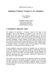
Instantaneous release problems in natural rivers ... - MANHAZ
Instantaneous release problems in natural rivers ... - MANHAZ
Instantaneous release problems in natural rivers ... - MANHAZ

Create successful ePaper yourself
Turn your PDF publications into a flip-book with our unique Google optimized e-Paper software.
<strong>Instantaneous</strong> <strong>release</strong> <strong>problems</strong> <strong>in</strong><br />
<strong>natural</strong> <strong>rivers</strong>: experiments and<br />
alarm models.<br />
Paweł M. Rowiński<br />
Institute of Geophysics<br />
Polish Academy of<br />
Sciences<br />
Warsaw, Poland<br />
orkshop on Modell<strong>in</strong>g of pollutant transport <strong>in</strong> water bodies for decision mak<strong>in</strong>g<br />
ay 30 - 31, 2005, Centre of Excellence <strong>MANHAZ</strong>
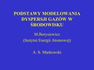
Natural Rivers – Plan View<br />
• Straight<br />
• S<strong>in</strong>uous<br />
• Meander<strong>in</strong>g<br />
•Braided<br />
• Anabranch<strong>in</strong>g<br />
• Anastomos<strong>in</strong>g<br />
Morphology
River<strong>in</strong>e wetlands<br />
• River<strong>in</strong>e wetlands form as l<strong>in</strong>ear strips,<br />
generally parallel<strong>in</strong>g river & stream<br />
channels.<br />
• They are found at lower elevations <strong>in</strong> a<br />
floodpla<strong>in</strong> and tend to be more frequently<br />
<strong>in</strong>undated and for a longer duration than<br />
areas at slightly higher elevation.
Clean<strong>in</strong>g or<br />
Filter<strong>in</strong>g pollutants<br />
From surface waters<br />
River<strong>in</strong>e Wetlands<br />
Accumulation of harmful substances<br />
May become disastrous<br />
Habitat for wildlife &<br />
plants<br />
e.g. wildlife<br />
mortality!
AIMS<br />
• understand<strong>in</strong>g of the mechanisms govern<strong>in</strong>g<br />
pollution transport <strong>in</strong> the river wander<strong>in</strong>g<br />
through a wetland area.<br />
• creation of respective mathematical models<br />
of the pollution transport <strong>in</strong> the stream as a<br />
start<strong>in</strong>g po<strong>in</strong>t
AIMS -CONTINUATION<br />
CONTINUATION<br />
• Evaluation of the threats by an accidental<br />
<strong>release</strong> of the pollutants at the downstream<br />
locations <strong>in</strong> a complex multi-channel river<br />
system.<br />
• Particular aim: determ<strong>in</strong>ation of<br />
concentration pattern of accidental <strong>in</strong>puts of<br />
toxic materials with<strong>in</strong> the Narew National<br />
Park.
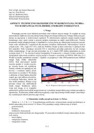
The Upper Narew River<br />
with<strong>in</strong><br />
the Narew National Park<br />
Legend<br />
Kurowo<br />
Radule<br />
Waniewo<br />
Kruszewo<br />
Łupianka Stara<br />
boundary of NNP protective zone<br />
river<br />
boundary of Narew National Park<br />
0 2 050 4 100 8 200<br />
Meters<br />
Rzędziany<br />
Izbiszcze<br />
Łapy<br />
Bok<strong>in</strong>y<br />
Uhowo<br />
Topilec<br />
Choroszcz<br />
Baciuty<br />
Suraż
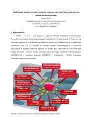
Narew – anastomos<strong>in</strong>g river<br />
In case of the Upper Narew we<br />
deal with the multi-channel system<br />
on a flood pla<strong>in</strong> but <strong>in</strong> contrast to<br />
the typical braided <strong>rivers</strong>, they are<br />
represented by relatively small<br />
slopes.<br />
Anastomos<strong>in</strong>g multichannel streams<br />
evelop when vegetation has stabilized the<br />
ream banks and the channel.
There are islands between<br />
various channels seen at normal<br />
stages of water but from time<br />
to time they are flooded for<br />
the period of days and weeks.
Methods<br />
• Tracer study <strong>in</strong> which a known mass of a<br />
conservative solute (Rhodam<strong>in</strong>e WT) is <strong>release</strong>d<br />
<strong>in</strong>to the stream.<br />
• Study consists <strong>in</strong> the exam<strong>in</strong>ation of the<br />
concentration versus time of the artificially<br />
<strong>release</strong>d dye at downstream stations and fitt<strong>in</strong>g<br />
appropriate models.<br />
• DEVELOPMENT OF MATHEMATICAL<br />
MODEL
Hydrological Survey<br />
• A precondition for a proper understand<strong>in</strong>g<br />
of the physical processes that occur <strong>in</strong> a<br />
river (and among them the processes<br />
govern<strong>in</strong>g the transport of pollutants) is a<br />
detailed recognition of hydrological and<br />
morphometric state with<strong>in</strong> the river channel<br />
and possibly on the floodpla<strong>in</strong>s.
Hydrological Survey urvey (NNP)<br />
• Description of channel network<br />
• Streamwise velocity field<br />
• Discharges at selected cross-sections<br />
• Water surface slopes (along whole river<br />
reach and local) and bed slope<br />
• Hydraulic and topographic characteristics
GPS SURVEY<br />
RESULTS
Geodesy
Terra<strong>in</strong> diversity
Velocity measurements
Example of velocity distribution
x 1<br />
Hydraulics computations<br />
h 1<br />
z v 1 (x,y)<br />
x<br />
y<br />
Q<br />
z<br />
x 2<br />
x<br />
h 2<br />
v 2 (x,y)<br />
y<br />
x
Cross-section Cross section survey layout<br />
LEGEND<br />
HG44<br />
G43<br />
HG42<br />
HG41<br />
0 330 660 1 320<br />
Meters<br />
HG40<br />
Floodpla<strong>in</strong> limits<br />
HG39<br />
HG38<br />
HG37<br />
Cross-section
elevation [m a.sl.]<br />
124<br />
123<br />
122<br />
121<br />
120<br />
119<br />
118<br />
117<br />
116<br />
115<br />
The generated, obta<strong>in</strong>ed from a field survey,<br />
and simplified G5 cross-section<br />
cross section<br />
G6<br />
generated<br />
measured<br />
simplified<br />
0 200 400 600 800 1000 1200 140<br />
distance [m]
Flood wave rout<strong>in</strong>g through the<br />
Narew river - computations
Unsteady flow rout<strong>in</strong>g<br />
through the ma<strong>in</strong> channel
Dynamic wave model for synthetic hydrograph<br />
Qt ( ) = Q + Qexp( −( t−T) /( T −T))(<br />
t/ T)<br />
discharge [m3/s]<br />
35<br />
30<br />
25<br />
20<br />
15<br />
10<br />
5<br />
0<br />
b 0<br />
p g p p<br />
HG0<br />
HG18<br />
HG27<br />
G33<br />
HG37<br />
HG44<br />
0 100 200 300 400 500 600 700 800 900 1000 1100 1200<br />
( T /( T −T<br />
))<br />
p g p
discharge [m3/s]<br />
50<br />
40<br />
30<br />
20<br />
10<br />
0<br />
Flood wave – spr<strong>in</strong>g 2004<br />
HG0<br />
HG18<br />
HG27<br />
G33<br />
HG37<br />
HG44<br />
0 100 200 300 400 500 600 700 800 900 1000
Unsteady flow rout<strong>in</strong>g of<br />
overbank flows
water level [m a.s.l.]<br />
117<br />
116.5<br />
116<br />
115.5<br />
115<br />
114.5<br />
114<br />
113.5<br />
Recorded and simulated water elevations<br />
at Bok<strong>in</strong>y village cross-section<br />
cross section<br />
measured<br />
simulated<br />
0 1000 2000 3000 4000 5000<br />
time [h]
Maximum water levels at the cross-sections cross sections HG18<br />
120<br />
118<br />
116<br />
Elevation [m above sea level]<br />
maximum water level<br />
1980a<br />
1978<br />
1980b<br />
1981<br />
1979<br />
114<br />
0.00 206.75 413.50 620.25 827.00<br />
HG18<br />
Distance [m]
looded area maps for<br />
e typical<br />
lood ood wave recorded <strong>in</strong> 1978<br />
LEGEND<br />
1978<br />
0 500 1 000 2 000<br />
!<br />
HG27<br />
!<br />
G24<br />
!<br />
!<br />
G28<br />
G23<br />
!<br />
HG44<br />
HG22<br />
!<br />
!<br />
G21<br />
!<br />
!<br />
G43 HG41<br />
!<br />
!<br />
!<br />
!<br />
!<br />
HG42 HG40<br />
HG42<br />
!<br />
HG38<br />
! HG31<br />
G29 G30<br />
HG18<br />
!<br />
!<br />
!<br />
!<br />
HG16<br />
!<br />
G15<br />
G14<br />
HG11<br />
!<br />
G10<br />
!<br />
!<br />
!<br />
G9<br />
G8<br />
G33<br />
!<br />
G7<br />
!<br />
!<br />
!<br />
G6<br />
HG5<br />
HG36<br />
HG34<br />
!<br />
!<br />
HG37<br />
G3 !<br />
G2<br />
!
Dye tracer test<br />
• The method of <strong>in</strong>stantaneous <strong>in</strong>jection of the<br />
tracer was applied<br />
• The dye <strong>release</strong> consisted of 20 liters of 20%<br />
solution of Rhodam<strong>in</strong>e WT at the cross-section<br />
just downstream of the bridge at Suraż.<br />
• Concentrations were measured at six transects<br />
(3.62 km, 8.34 km, 9.01 km, 9.23 km, 13.58 km,<br />
and 16.83 km). First cross-section was established<br />
at a distance at which 1D conditions were<br />
supposed to be achieved.
o ga<strong>in</strong> more understand<strong>in</strong>g<br />
recognition of hydraulics<br />
conditions is needed<br />
Tracer test
Spread<strong>in</strong>g of Rhodam<strong>in</strong>e WT at the early stage<br />
where lateral mix<strong>in</strong>g occurs
The stage where the tracer is mixed across
Variation of concentration with time at the<br />
cross-sections cross sections downstream of the <strong>in</strong>jection<br />
c(t)<br />
800<br />
700<br />
600<br />
500<br />
400<br />
300<br />
200<br />
100<br />
0<br />
2-N<br />
3-N<br />
5-N<br />
6-N<br />
7-N<br />
0 5 10 15 20 25 30 35 40<br />
time [hours]
Why the mathematical<br />
treatment of pollution transport<br />
offers so many difficulties?
50<br />
45<br />
40<br />
35<br />
30<br />
25<br />
20<br />
15<br />
10<br />
5<br />
0<br />
U [cm/s]<br />
Vertical 13 y = 4 cm<br />
Firstly:<br />
River flow turbulence<br />
Test 2 U = 19.4 cm/s<br />
Test 3 U = 6.1 cm/s<br />
Test 1 U = 38.5 cm/s<br />
0 20 40 60 80 100 120 140 160 180<br />
t [s]
Secondly:<br />
Extremely complex geometry<br />
especially <strong>in</strong> wetland areas
Model<strong>in</strong>g concept
Flow Q<br />
Lateral<br />
<strong>in</strong>flow<br />
Ma<strong>in</strong> channel<br />
Exchange due to<br />
transient storage<br />
Transient<br />
storage<br />
Small <strong>rivers</strong><br />
Ma<strong>in</strong> channel<br />
wetlands<br />
Transient storage<br />
Side pockets,<br />
hyporheis stratum,<br />
bed irregularities<br />
Downstream<br />
transport<br />
Advection and<br />
dispersion<br />
Outflow
Storage zone
Models of pollution transport<br />
Steady and uniform flow conditions<br />
2<br />
∂C ∂C ∂ C ε<br />
+ U − D = C 2<br />
D −C<br />
∂t ∂x ∂x<br />
T<br />
Steady but non-uniform flow conditions<br />
Transient storage<br />
zones<br />
Ma<strong>in</strong> channel<br />
∂C ∂C<br />
1 ∂ ⎛ ∂C<br />
⎞ ε<br />
+ u − ⎜ DA ⎟ =<br />
∂t<br />
∂x<br />
A ∂x<br />
⎝ ∂x<br />
⎠ T<br />
∂C 1<br />
=<br />
∂t<br />
T<br />
( C − )<br />
D CD<br />
( )<br />
( C C)<br />
D −
Schematic representation of the solution<br />
method – splitt<strong>in</strong>g technique<br />
TRANSPORT<br />
<strong>in</strong>put output<br />
<strong>in</strong>put<br />
advection<br />
output<br />
advection dispersion storage zone<br />
advection<br />
advection -<br />
dispersion<br />
output<br />
upw<strong>in</strong>d<br />
scheme<br />
dispersion<br />
Crank - Nicholson<br />
scheme<br />
storage<br />
zones<br />
Runge – Kutta<br />
method<br />
output
Identification of model<br />
parameters
Optimization Procedure 1 – based on frequency<br />
response function<br />
⎡ 2 2 3<br />
U x 2 4DεTω 4 D( T ω + ω+ εω)<br />
⎤<br />
H( x, iω) = exp⎢ x− U + + i<br />
2 2 2 2 ⎥<br />
⎢⎣ 2D 2D T ω + 1 T ω + 1 ⎥⎦<br />
Optimization procedure on the reach by reach basis<br />
with specially designed objective function compar<strong>in</strong>g<br />
the reverse of Fourier transformation of function H and<br />
the measured concentrations.
Another formulation of optimization problem<br />
Criterion for parameters derivation<br />
[ ] ( ) ( ) 2<br />
TH<br />
⎧ K<br />
⎪ ⎫⎪<br />
m<strong>in</strong> ⎨FuD , , ε,<br />
T = ∑ ∫ ⎡⎣Cx, t −Cx,<br />
t⎤⎦ dt⎬<br />
⎩ ⎭<br />
m k k<br />
uD , , ε , T<br />
⎪ k = 2 0<br />
⎪<br />
Constra<strong>in</strong>ts for the<br />
problem<br />
Water cont<strong>in</strong>uity equation<br />
( )<br />
X ≤ X x ≤ X<br />
m<strong>in</strong> max<br />
Q= uA
Control Random Search<br />
Start of computations – set of po<strong>in</strong>ts<br />
Determ<strong>in</strong>ation of the best xL and<br />
the worst xH from the given set<br />
Formation of a simplex conta<strong>in</strong><strong>in</strong>g x L<br />
xn+1 - result: new po<strong>in</strong>t xW Reflection of the last po<strong>in</strong>t from simplex<br />
Replacement of x H by x W<br />
Stop criterion<br />
F − F x<br />
sr<br />
( L ) < ε<br />
x 1<br />
constant values of objective function<br />
optimum<br />
simplex 3<br />
simplex 2<br />
simplex 1<br />
The search<strong>in</strong>g rule for the doma<strong>in</strong><br />
of the objective function by means<br />
of simplex method<br />
x 2
Dead-zone Dead zone model parameters –<br />
E L [km 2 /h]<br />
ε<br />
T[h]<br />
U a [km/h]<br />
Parameters<br />
[0-N,2-N]<br />
0.0027<br />
0.0920<br />
0.4530<br />
0.5200<br />
Upper Narew<br />
[2-N,3-N]<br />
0.0220<br />
0.0120<br />
0.6550<br />
1.8400<br />
[3-N,5-N]<br />
0.0051<br />
0.7920<br />
11.2570<br />
0.4880<br />
Sections<br />
[5-N,6-N]<br />
0.0338<br />
0.3690<br />
7.0706<br />
1.6200<br />
[6-N,7-N]<br />
0.0034<br />
0.2260<br />
0.9030<br />
0.7800<br />
[0-N,7-N]<br />
0.0120<br />
0.1020<br />
1.440<br />
0.9190
Examples of measured and dead-zone dead zone<br />
model results<br />
0,40<br />
0,35<br />
0,30<br />
0,25<br />
0,20<br />
0,15<br />
0,10<br />
0,05<br />
0,00<br />
Dimensionless concentration<br />
10 15 20 25 30 35 40<br />
time [hours]<br />
experimental data<br />
model
Cont<strong>in</strong>uation of studies<br />
• Computations under flood conditions, also<br />
when the entire floodpla<strong>in</strong> is <strong>in</strong>undated.<br />
• The above requires a very good recognition<br />
of the topography of the entire valley<br />
• Flow computations based on CCHE models<br />
– currently conducted
Conclud<strong>in</strong>g remarks<br />
• It is shown that because of the asymmetric nature<br />
of all the observed breakthrough curves, the<br />
temporary storage of the admixture plays a crucial<br />
role <strong>in</strong> the analyses of the pattern of its spread <strong>in</strong><br />
the multi-thread river system. This reflects the<br />
<strong>in</strong>teractions with the adjacent wetland areas (high<br />
values of ε<br />
<strong>in</strong> the model)
Conclud<strong>in</strong>g remarks -cont cont<br />
• A tracer test def<strong>in</strong>itely facilitates the analyses and<br />
quantification of the hydrodynamic and also<br />
chemical processes <strong>in</strong> surface waters, particularly<br />
<strong>in</strong> such complex environment as the Upper Narew.<br />
Because of its complete safeness for the<br />
environment such method is recommended as a<br />
tool for the recognition of the system behavior.
THANK YOU FOR<br />
YOUR ATTENTION