Introduction to vector and tensor analysis

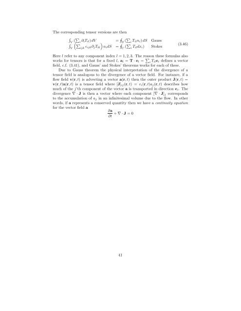
The corresponding tensor versions are then
V (i
∂iTil) dV =
nidS =
V
ijk ɛijk∂jTkl
S (
i Tilni) dS Gauss
C (
i Tildxi) Stokes
(3.46)
Here l refer to any component index l = 1, 2, 3. The reason these formulas also
works for tensors is that for a fixed l, al = T · el =
i Tilei defines a vector
field, c.f. (3.41), and Gauss’ and Stokes’ theorems works for each of these.
Due to Gauss theorem the physical interpretation of the divergence of a
tensor field is analogous to the divergence of a vector field. For instance, if a
flow field v(r, t) is advecting a vector a(r, t) then the outer product J(r, t) =
v(r, t)a(r, t) is a tensor field where [J]ij(r, t) = vi(r, t)aj(r, t) describes how
much of the j’th component of the vector a is transported in direction ei. The
divergence ∇ · J is then a vector where each component [∇ · J]j corresponds
to the accumulation of aj in an infinitesimal volume due to the flow. In other
words, if a represents a conserved quantity then we have a continuity equation
for the vector field a
∂a
+ ∇ · J = 0
∂t
41