ThC03.1

2005 American Control Conference
June 8-10, 2005. Portland, OR, USA
Time-Dependent Dynamics in
Networked Sensing and Control
Justin R. Hartman, Michael S. Branicky, and Vincenzo Liberatore
Electrical Engineering and Computer Science Department
Case Western Reserve University, Cleveland, OH 44106
jjhartman@ra.rockwell.com, {mb,vincenzo.liberatore}@case.edu
Abstract— A networked sensing and control system (NSCS)
combines networked sensors with control and actuation units
so as to control a physical environment. An NSCS can effectively
use sensing and control signals only if those signals are
delivered on time. The paper analyzes the behavior of an NSCS
as a function of network real-time service. In particular, we
consider the range of effective sampling periods and network
delays that lead to stability for the controlled physical plant.
A high-level conclusion is that the actual stability region is
affected by the time-dependent behavior of packet delays and
losses and can differ from an idealized stability region derived
from an aggregate view of the loss and delay processes.
I. INTRODUCTION
A networked sensing and control system (NSCS) combines
networked sensors with control and actuation units so
as to control a physical environment (Fig. 1). Applications
are far-reaching and include, for example, industrial automation
and distributed instrumentation [1]. A fundamental
problem in NSCS is that sensor and control signals are
useless or dangerous if they are delivered too late. In
particular, a late control can jeopardize the stability, safety,
and performance of the controlled physical environment. As
a result, the physics of an NSCS critically depends on the
real-time network behavior.
A broad research objective is to establish a methodology
and the theoretical underpinnings of networked control [8].
In this paper, we analyze and simulate a representative
physical system on simple topology. Our primary objective
is to ascertain to what extent the complexity of time-varying
network dynamics can be incorporated into a controltheoretical
model. The paper focuses on packet-switched
sensor networks because they are in widespread use in
industrial automation and because the analysis is simpler
than in an ad-hoc network.
In Section II, we introduce the NSCS that will be analyzed
throughout the paper. Section III frames the main
analytical properties of this NSCS, including the stability
region and the traffic locus. In Section IV, we describe our
co-simulation methodology. Section V gives the results of
our co-simulations. Section VI concludes the paper.
For a fuller listing of works in the NSCS realm, consult
the bibliography and the references contained herein, the
thesis [5] from which this paper is condensed, or consult
the papers and resources provided online in [8].
0-7803-9098-9/05/$25.00 ©2005 AACC
2925
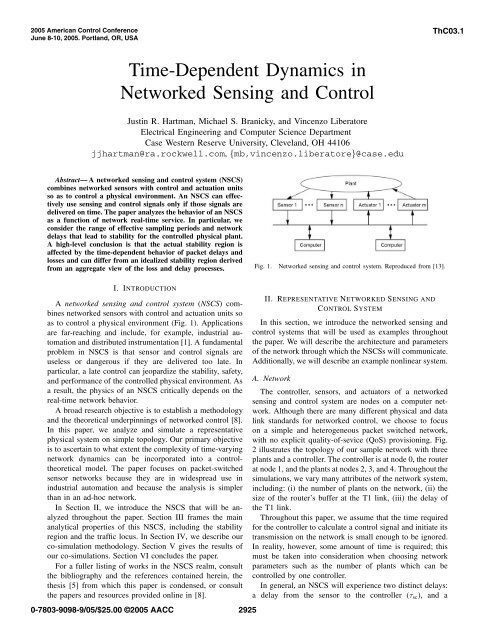
Fig. 1. Networked sensing and control system. Reproduced from [13].
II. REPRESENTATIVE NETWORKED SENSING AND
CONTROL SYSTEM
ThC03.1
In this section, we introduce the networked sensing and
control systems that will be used as examples throughout
the paper. We will describe the architecture and parameters
of the network through which the NSCSs will communicate.
Additionally, we will describe an example nonlinear system.
A. Network
The controller, sensors, and actuators of a networked
sensing and control system are nodes on a computer network.
Although there are many different physical and data
link standards for networked control, we choose to focus
on a simple and heterogeneous packet switched network,
with no explicit quality-of-sevice (QoS) provisioning. Fig.
2 illustrates the topology of our sample network with three
plants and a controller. The controller is at node 0, the router
at node 1, and the plants at nodes 2, 3, and 4. Throughout the
simulations, we vary many attributes of the network system,
including: (i) the number of plants on the network, (ii) the
size of the router’s buffer at the T1 link, (iii) the delay of
the T1 link.
Throughout this paper, we assume that the time required
for the controller to calculate a control signal and initiate its
transmission on the network is small enough to be ignored.
In reality, however, some amount of time is required; this
must be taken into consideration when choosing network
parameters such as the number of plants which can be
controlled by one controller.
In general, an NSCS will experience two distinct delays:
a delay from the sensor to the controller (τsc), and a

Fig. 2. Network topology with three plants.
delay from the controller to the actuator (τca). Each can
be analyzed using Eqs. (10) and (11) to find the bounds in
which the the sensor-to-controller or controller-to-actuator
delay will remain. Figure 3 illustrates the timing of the
packets on an NSCS, including the sensor-to-controller and
controller-to-actuator delays.
Fig. 3. Delay timing diagram for an NSCS. Reproduced from [14].
location, with motion to the right being positive). For more
details about the inverted pendulum, including Matlab code,
see [3], [9], [11].
Fig. 4. Cartoon of inverted pendulum system. Modified from [11].
Once the system has been linearized, we can express it
in state-space form, as in Eq. (2).
⎡ δx
δt
δ ˙x
⎢ δt
⎣ δφ
δt
δ ˙ ⎤ ⎡
0 1 0 0
⎥ ⎢ 0 0 0 0
⎦ = ⎣ 0 0 0 1
φ
3g
0 0
δt
4L − 3BR 4ML2 ⎤ ⎡ ⎤ ⎡
x 0
⎥ ⎢ ˙x ⎥ ⎢ 1
⎦ ⎣ φ ⎦ + ⎣ 0
˙φ − 3
⎤
⎥
⎦ u.
4L
(2)
When we sample a continuous-time system with a constant
sampling period h, the resulting discrete-time system
can be described by
where
x [k +1]=Φx [k]+Γu [k] , (3)
Φ=e Ah , Γ=
h
0
e As ds B. (4)
Assuming the full state is available through sensors,
a linear controller of the form u[k] = −Kx[k] can be
designed to meet stability or performance objectives of the
the overall, closed-loop system:
x [k +1]=Φx [k] − ΓKx[k] =(Φ− ΓK)x [k] . (5)
B. Control System
We introduce and describe the system which will be used
as an example: an inverted pendulum. It consists of a single
point mass on the end of a rod, swinging freely from a cart
on a track. Fig. 4 presents a cartoon of this system. The
equations of motion for the inverted pendulum are:
¨φ + 3BR
4ML2 ˙ φ − 3g
There are well-known methods (pole placement, LQR, etc.)
thatmaybeusedtodesignK [4]. In this paper, we will
primarily be concerned with the case where K is chosen
such that the closed-loop system matrix Φ − ΓK is Schur
(i.e., all its eigenvalues have magnitude less than one).
3
sin φ = − ¨x, (1)
4L 4L
where BR is the coefficient of friction of the pivot joint, M
is the mass of the weight at the end of the rod, L is the length
of the rod, and g is the gravitational constant. The input
(control signal, u) to the cart-mass system is the acceleration
¨x = u of the cart, and the outputs are the angle of the
pendulum, φ (as measured from the “up” vertical position,
with clockwise rotation being positive), and the position of
III. ANALYSIS
A. Constant Network Delays
For networked sensing and control systems with fixed
delays, we can analyze the system by reformulating the
system matrices. Since the actuation of the system occurs at
some time τ after the controller has calculated the control
signal, we must revise the system model to account for
this delay. For delays less than one sampling period, and
assuming a constant sampling period h, we can model the
system as follows [4]:
the cart on the track, x (as measured from an arbitrary zero x [k +1]=Φx [k]+Γ0 (τ) u [k]+Γ1 (τ) u [k − 1] , (6)
2926

where
Φ=e Ah h−τ
, Γ0 (τ) = e As h
Bds, Γ1 (τ) =
0
h−τ
e As B ds.
(7)
By augmenting the system state space with the previous
control signal value, we obtain ˜x [k +1]= Øx [k]+ ˜ Bu[k] ,
where
à =
Φ Γ1
0 0
, ˜ B =
Γ0
1
L∈L
, ˜x [k] =
x [k]
u [k − 1]
.
(8)
The delay for all packets in transit on the links in L will be
bounded by [τmin,τmax].
C. Varying Delay and Effective Sampling Period
The effective sampling period of an NSCS is the average
sampling period of the NSCS over a period of time, taking
into account all of the packet losses:
th
heff (t) = , (12)
t − hd (t)
where h is the nominal sampling period in seconds, and
d (t) is the total number of packets belonging to the plant
under observation dropped before time t.
If all the packets dropped on a link are due to oversaturation
of the network, then we can use aprioriknowl edge of the network topology, link speeds, sampling periods,
and data packet sizes to calculate the rate, r, at which control
packets will be transmitted:
ηL
r =min , 1 , (13)
8ET
The stability of the system in Eq. (5) in an NSCS setting,
sampled periodically with period h and subject to fixed
delay τ, can be assessed by testing the Schur-ness of the
matrix
à − ˜ B [K 0] . (9)
For delays greater than one sampling period, a similar
process of augmenting the state space with more delayed
control signals (e.g. u[k − 2], ..., u[k − n]) can be used. For
a fuller treatment of these techniques, see [13], [4].
In special cases (e.g., scheduled, no-collision transmissions
on a private network), these methods are applicable.
However, in NSCS involving the Internet, delays are in
general unpredictable [6].
B. Network Bottlenecks
Two of the primary difficulties in the analysis and design
of networked sensing and control systems are packet loss
and transmission delays. Some amount of delay is inherent
in the data transmission across a network, and does not
change; the portion of network-induced delay which can
vary, as well as the phenomena of packet losses, are a
result of collisions and queuing at intermediate nodes on
a network. We investigate the primary causes of data loss
and delay here.
In network devices (routers, switches, and hubs), the
size of the link storage buffer is configurable. Hence, the
maximum delay possible of an NSCS packet (traveling over
asetofLlinks from source to destination) is directly related
to the size of the link buffers:
τmax =
δL +
L∈L
8P (βL
+1)
,
ηL
(10)
where δL is the fixed link delay of link L, P is the packet
size in bytes, βL is the buffer size of link L in number of
packets, and ηL is the link speed of link L in bits per second.
(We assume for simplicity that all packets have the same size
P . If the buffer size is expressed in bytes rather than the
number of packets, one can simply use the packet size P
to determine βL.) Eq. (10) predicts that the maximum link
delay increases with the buffer size. Of course, a smaller
buffer also implies a larger number of packet losses.
The minimum delay for a network path is
τmin =
δL + 8P
where ηL is the link speed of the bottleneck link (in bits per
second), and ET is the number of bytes expected to arrive
at the bottleneck link during one second of operation. For
periodic traffic sources, we can replace ET in Eq. (13) with
asum:ET =
. (11)
ηL
Si
i∈N hi ,whereSiisthesize of the periodic
packet from the ith node (in bytes), hi is the transmission
period of the ith node, and N is the set of all periodic nodes
on the network.
Thus, given an expected usage pattern of the network, including
all NSCSs and other regular periodic traffic sources,
one can calculate an expected value of the transmission rate.
Further, if we are given the transmission rate r, we can also
calculate the effective sampling period, heff:
heff = h
r =max
8h i∈N
ηL
Si
hi ,h , (14)
where h is the sampling period for which the plant was
designed.
D. Sampling Period and Delay Stability Region
For an ideal networked sensing and control system with
no data loss and fixed delays, we can derive bounds on the
sampling period and delay under which the system remains
stable. By varying the sampling period and the constant
delay of the system and testing the stability of the resulting
system matrix (see Eq. (9)), we can plot the boundary of a
region of stability, which we call the sampling period and
delay stability region (SPDSR). This idea was developed
by Zhang et al. in [14], [13]; a generalized algorithm
for discovering the SPDSR given continuous-time system
matrices and a discrete-time feedback matrix is given in
[5].
2927

E. Traffic Locus
A traffic locus is a locus of points describing, in the same
sampling period and delay space as the stability regions,
the theoretically possible points of effective sampling period
and network-induced delay for a single plant, as a function
of the amount of traffic on the network.
At all times, the packet delays on a network will be
bounded by [τmin,τmax] from Eqs. (10) and (11). As long
as the amount of traffic remains below the bandwidth of the
network, the effective sampling period of a plant will be
its actual sampling period, and the delay will remain fixed
at τmin. However, once the amount of traffic exceeds the
network bandwidth, the delay will remain fixed at τmax and
the effective sampling period will increase. For networks
where all nodes are periodic traffic sources, we can express
the traffic locus as
T (heff) =
τmin
h eff , for heff = h,
τmax
h eff , for heff >h,
(15)
where h is the sampling period for which the plant was
designed, and heff can be calculated from Eq. (14) for
different amounts of network traffic.
IV. CO-SIMULATION METHODOLOGY
A. Network
In order to simulate a networked sensing and control
system, the simulation of the dynamics of the state-space
equations of a control system was combined with the simulation
of a network topology into a single ns-2 simulation
script. This script utilizes the network components of ns-2
to simulate network dynamics, such as the transmission,
queuing, forwarding, and receipt of packets, as well as
any network cross-traffic, such as FTP flows; the script
also utilizes the Agent/Plant extension [2], [7] to simulate
the sampling, control, and actuation of the control system
components. The dynamics of each plant were simulated
inline by first-order Euler approximations [5].
For these simulations, the controller is connected directly
to a router by means of a T1 line, which has a bandwidth of
1.5 Mbps and a fixed link delay of 1 ms. Every other node on
the network is a plant, which contains both the sensors for
full-state feedback and the actuator for the control signal.
All plant nodes are connected to the router via 10 Mbps
links, with fixed link delays of 0.1 ms.
To illustrate the possible asymmetry of network delays,
consider the sample network topology, where each link has
a link buffer size of 50 packets. Using Eqs. (10) and (11),
we discover that the sensor-to-controller and controller-toactuator
delays are bounded by
1.494ms ≤ τsc ≤ 17.770ms,
1.494ms ≤ τca ≤ 3.936ms.
In addition, if faster nodes flood the downstream T1 link
to the controller, then the sensor-to-controller delay will be
fixed at τsc, max. The controller, however, cannot flood the
2928
faster outbound links; therefore, the controller-to-actuator
delay will be fixed at τca, min.
In addition to varying the network attributes listed above,
we may wish to randomize or fix the scheduling of the
plants’ samples on the network. When we do not randomize
the system sampling times, each plant uses the same
sampling period for which it was designed, and the plants’
samples are scheduled to be equidistant in time from one
another within the sample period. More precisely, we choose
the sampling period and sampling times of each plant be
hi = H, ti [k] =
k +
i − 1
N
hi, (16)
where i ∈{1,...,N}. Here,hi is the sampling period of
the i th plant, ti [k] is the absolute time of the k th sample of
the i th plant, H is the sampling period for which the system
was designed, and N is the total number of plants. When
the sampling of the plants is fixed according to Eq. (16), it
establishes a periodicity among the samples of all plants. It
also provides the same amount of bandwidth to each plant
on the network.
For no “overlap” of transmission times, one must assume,
in addition to Eq. (16), that the transmission time of each
packet is less than the bandwidth devoted to each packet.
More precisely,
P
η
H
< , (17)
N
where P is the size of the periodic NSCS packet, η is
the bandwidth of the network path, and H and N are
as before. If this assumption is not true, then we say the
resulting network is over-commissioned; that is, the nodes
commissioned on the network require more bandwidth than
the network is able to provide. Such a situation will result
in packet losses.
When the sampling times are randomized, each plant
(with the exception of the first plant, which we are observing)
chooses a sampling period up to 20% greater
or less than the designed sampling period. In addition,
the scheduling of the plants is randomized throughout the
sampling period. Assuming there is no jitter in the plants’
timing, we choose the sampling period and sampling times
of the first plant in the same way as the non-randomized
case of Eq. (16). Then for each plant i>1, we choose
two random variables, ρi ∈ [0.8, 1.2] and ψi ∈ [0, 1), which
represent the skew of the sampling period and the skew
of the initial sample time, respectively, from a uniform
distribution on their intervals. We then fix each plant’s
sampling period and sampling times as follows:
hi = ρiH, ti [k] =(k + ψi) hi. (18)
When the sampling of the plants is randomized, it eliminates
the periodicity found in the non-randomized sample
schedules of Eq. (16); this better mirrors the real-world case
where clock asynchronicity and skew cause aperiodic traffic
sequences. Additionally, individual plants on the network

may be effectively allocated more or less bandwidth than
the non-randomized case.
B. Control System
The system contains nonlinearities, and we will linearize
it for ease of analysis. However, we will simulate both
linear and nonlinear system equations in order to observe
the effects of the nonlinearity in the simulation results.
We have chosen values for the inverted pendulum system
parameters: g = 9.8066 m/s2 , M = 8 kg, L =
0.125 m, BR =0.1. These parameters correspond to reasonable
values in a physical implementation. The open loop
system is unstable (poles at 0, 0, and ±8) and controllable.
We designed a full-state feedback controller for the inverted
pendulum system to sample at a constant rate of 50 ms,
which is used in the remainder of this paper:
K = −0.6673 −1.1453 −19.4454 −2.4364 .
(19)
This yields system poles at 0.6809 ± 0.0086i and 0.9647 ±
0.0340i for the closed-loop system matrix Φ − ΓK. See[5]
for details. For all simulations that follow, we use the initial
condition (x, ˙x, φ, ˙ φ)=(0, 0, −.2095, −0.0977).
While the analytic stability region can be informative,
we wish to discover the stability region of a plant using
the effective sampling period from Eq. (14). In order to
do this, we must cause the NSCS to drop packets by
over-saturating the network’s bandwidth. Since the effective
sampling period is directly proportional to the number of
plants on the network, and the maximum delay of the link
path is directly related to the router queue size, we can
vary the number of plants and the router queue size to test
different points in the sample space.
C. Implementation
Simulations using the ns-2 network simulator used
version 2.26, running in Cygwin version 1.5.5. Matlab-based
calculations were done in Matlab 6.5.0.180913a Release
13. In all simulation results, we only tracked the state and
output of the first plant in Fig. 2 (boxed node 2). For all
other plants, only the network events are simulated; their
dynamics are symmetric and hence not simulated, in order
to conserve processor time during simulation.
V. CO-SIMULATIONS
A. Baseline
As a first step to understanding the influence of the control
network on an NSCS, we compare the performance of the
“ideal” NSCS against that of the non-networked, discretetime
system. We have simulated the inverted pendulum
system with only one plant on the network, sampling at
50 ms, with no additional cross-traffic. Fig. 5 illustrates the
system state of the baseline NSCS vs. the non-networked
inverted pendulum system.
The baseline NSCS experiences small and constant
sensor-to-controller and controller-to-actuator delays (about
2929
Phi (radians)
0.2
0.1
0
−0.1
Phi
−0.2
Non−Networked
Baseline NCS
0 5 10 15
Time (s)
Phi dot (radians / s)
4
2
0
−2
−4
Phi by Phi dot
Non−Networked
Baseline NCS
−0.2 −0.1 0
Phi (radians)
0.1 0.2
X (meters)
X dot (m / s)
0
−0.02
−0.04
−0.06
−0.08
−0.1
−0.12
0.5
−0.5
X
0 5 10 15
Time (s)
1
0
X by X dot
Non−Networked
Baseline NCS
Non−Networked
Baseline NCS
−1
−0.1 −0.05 0
X (m)
0.05 0.1
Fig. 5. Simulation of baseline inverted pendulum system.
1.5 ms each) due to the fixed propagation and transmission
delays along the network paths. These delays cause the
state of the inverted pendulum system to differ from that of
the non-networked system at the same point in time. This
difference in system state causes a difference in the control
signal that is applied to the system.
B. Many Plants
In the baseline NSCS simulations, the only nodes communicating
on the network are the controller and the plant
under observation. This configuration uses little of the
system bandwidth, as the two nodes only exchange 64-byte
packets every 50 ms (using 10 Kbps, which is approximately
0.65% of the available bandwidth). In order to use more of
the network bandwidth, we will simulate the system with
147 NSCS plants communicating with the controller, which
will utilize the total amount of bandwidth available on the
T1 line. We fix the sample scheduling of the plants on the
network according to the non-randomized scheme of Eq.
(16). The performance of the inverted pendulum system
with this configuration is very similar to that of the baseline
system (data not shown).
When 147 plants communicate on the network, the bandwidth
of the T1 line is slightly exceeded. Because of that,
some sensor-to-controller packets are lost. Fig. 6 shows the
control signal of this system, as well as the number of
packets in the router queue, the number of packets lost at the
T1 line buffer, and the sensor-to-controller and controllerto-actuator
delays. As the queue begins to fill, the sensorto-controller
delay increases as incoming packets must wait
for the queue to empty. Once the queue has filled, packets
begin to be lost.
Although we are at the edge of bandwidth saturation, with
time-varying delays and some packet loss, the pendulum
shows performance similar to that of the baseline system.
C. Over-Commissioned Network
In order to better simulate and analyze packet loss,
we will study NSCSs which use more than the available
bandwidth. If the network is over-commissioned in this

Cart Acceleration
Number of Packets
5
0
−5
−10
Control Signal
−15
Baseline
147 Plants
−20
0 5 10 15
Time (s)
120
100
80
60
40
20
Total Dropped Packets
0
0 5 10 15
Time (s)
Delay (s)
Size (packets)
50
40
30
20
10
Router Queue Size
0
0 5 10 15
Time (s)
Sensor−to−Controller and Controller−to−Actuator Delays
0.02
0.015
0.01
0.005
Plant−to−Controller
Controller−to−Actuator
0
0 5 10 15
Time (s)
Fig. 6. Control signal, queue size, packet losses, and delays of the inverted
pendulum system with 147 plants.
way, the network is guaranteed to lose packets; by varying
the number of plants on the network, we can change the
amount of sensor-to-controller packets which make it to the
controller.
1) Non-Randomized Sample Scheduling: First, we fix the
scheduling of the plants on the network according the nonrandomized
schedule of Eq. (16). This evenly distributes the
amount of bandwidth per node. Fig. 7 illustrates the state
of the inverted pendulum system with 175 plants with nonrandomized
sensor scheduling. Even though we are only
slightly above the bandwidth of the T1 link, the system is
already marginally stable, because the inverted pendulum
system is sensitive to lost packets and long delays.
Phi (radians)
0.3
0.2
0.1
0
Phi
−0.1
Baseline
−0.2
175 Plants
0 5 10 15
Time (s)
Phi dot (radians / s)
5
0
−5
Phi by Phi dot
−0.2 0
Phi (radians)
Baseline
175 Plants
0.2
X (meters)
X dot (m / s)
0.05
0
−0.05
−0.1
0 5
Baseline
175 Plants
10 15
Time (s)
1
0.5
0
−0.5
−1
X
X by X dot
Baseline
175 Plants
−0.1 −0.05 0
X (m)
0.05 0.1
Fig. 7. Simulation of inverted pendulum on an over-commissioned
network.
Fig. 8 shows the control signal and network dynamics of
the inverted pendulum on an over-commissioned network.
Because of the amount of traffic, the router queue fills
quickly, and delays become high (18.23 ms) and nearly constant.
Also, approximately 8.4% of the sensor-to-controller
packets were lost.
2) Randomized Sample Scheduling: When the sampling
of the sensors is randomly scheduled according to Eq. (18),
the performance for the plant under observation can be
2930
Cart Acceleration
Number of Packets
Control Signal
15
10
5
0
−5
−10
−15
Baseline
−20
175 Plants
0 5 10 15
Time (s)
4000
3000
2000
1000
Total Dropped Packets
0
0 5 10 15
Time (s)
Delay (s)
Size (packets)
50
40
30
20
10
Router Queue Size
0
0 5 10 15
Time (s)
Sensor−to−Controller and Controller−to−Actuator Delays
0.02
0.015
0.01
0.005
Plant−to−Controller
Controller−to−Actuator
0
0 5 10 15
Time (s)
Fig. 8. Control signal, queue size, packet losses, and delays of the inverted
pendulum system on an over-commissioned network.
better or worse than when it is not randomized, depending
on the scheduled sampling times of the other plants.
The performance and stability of an NSCS on an overcommissioned
network with random scheduling is highly
dependent on the sensitivity of the NSCS to packet loss
and delay.
Fig. 9 illustrates the effective sampling of the first plant
versus the number of plants on the network and the link
buffer size. When the network is beyond saturation, the
buffer is overflowed, and therefore changing the buffer size
only increases the network-induced delay. However, as the
number of plants increases, both packet losses and the
effective sampling period increase.
Effective Sampling Period (s)
0.095
0.09
0.085
0.08
0.075
0.07
0.065
0.06
0.055
0.05
260
240
220
Number of Plants
200
180
Effective Sampling Period
160
0
20
40
Queue Size
Fig. 9. Effective sampling period vs. number of plants, link buffer size.
The effective sampling period of Eq. (14) is the expected
value over an infinitely long period, and with only periodic
traffic sources. If other bursty traffic sources intermittently
transmit on the network, then Eq. (14) under-estimates heff.
D. Stability Region
Fig. 10 (dotted line) is an analytical bound assuming a
fixed-delay system with a fixed sampling period; Fig. 10
(solid line) simulates this by fixing the central link delay to
60
80

τmin, and changing the actual sampling period of the plant.
Fig. 11 shows the analytical stability region from Fig. 10,
along with the experimental stability region discovered by
varying the buffer size and the number of plants on the
network, which change both the maximum delay τmax and
the effective sampling period heff.
Delay/Sampling Period
1
0.9
0.8
0.7
0.6
0.5
0.4
0.3
0.2
0.1
Stability Regions
Analytical
Experimental
0
0.04 0.06 0.08 0.1 0.12 0.14 0.16 0.18 0.2 0.22 0.24
Sampling Period (s)
Fig. 10. Sampling period and delay stability region for the inverted
pendulum: analytical and experimental from ns-2.
Delay / Sampling Period
1
0.9
0.8
0.7
0.3
0.2
0.1
Sample Point 1
Sample Point 3
Stability Regions
Sample Point 2
Analytical
Experimental
0
0.04 0.06 0.08 0.1
Sampling Period (s)
0.18 0.2 0.22 0.24
Fig. 11. Effective sampling period and maximum delay stability region
for the inverted pendulum: analytical and from ns-2.
Because the analytical stability region is defined in terms
of a constant sampling period and constant delay, it does not
truly represent an NSCS. Under real network conditions,
the delays of an NSCS will not be constant—they will
vary randomly due to other traffic and collisions. Likewise,
the sampling period will not vary linearly—rather, it will
jump between discrete values (h [k] ∈{h, 2h, 3h, ...}) for
varying numbers of consecutively dropped packets. The
theoretical stability region, then, is likely to be too liberal;
this suspicion is confirmed in the region of Fig. 11.
We have chosen three points in the sampling period and
delay space to illustrate the performance of the inverted
pendulum system. At Sample Point 1, there are 176 inverted
pendulum plants, and the T1 link has a buffer of 51 packets.
The resulting effective sampling period is 60.282 ms, and
the average delay is 18.342 ms. The performance of this
configuration is qualitatively the same as the baseline system
(data not shown).
At Sample Point 2, there are 411 inverted pendulum
plants on the network, and the T1 link buffer size is 38
packets. The resulting effective sampling period is 143.750
ms, and the average delay is 13.961 ms. Although this point
is still within the SPDSR for the fixed delay and sampling
period, the effective sampling period caused by packet loss
causes it to become unstable (not shown).
At Sample Point 3, there are 294 plants on the network,
and the T1 link buffer size is 180 packets. The resulting
effective sampling period is 101.014 ms, and the average
delay is 62.042 ms. This point is outside both stability
regions, and the system is clearly unstable; see Fig. 12.
Phi (radians)
Phi dot (radians / s)
5
4
3
2
1
0
Phi
−1
0 5 10 15
Time (s)
15
10
5
0
−5
−10
−15
Phi by Phi dot
−5 0
Phi (radians)
5
X (meters)
0
−5
−10
−15
−20
−25
−30
0 5 10 15
Time (s)
X dot (m / s)
4
2
0
−2
−4
X
X by X dot
−20 0
X (m)
20
Fig. 12. Inverted pendulum system simulation at Sample Point 3.
E. Traffic Locus
Since the delay in the sampling period and delay space
is a fractional delay, this line actually traces a curve in the
state space. Fig. 13 illustrates an example traffic locus for
the inverted pendulum system. In this sample system, the
queue size at the T1 boundary is fixed at 25; therefore,
the maximum delay (using Eq. (10)) is 9.681 ms, and the
minimum delay is 1.4744 ms. When the network bandwidth
is below 100% utilization, the system can be represented by
Sample Point 1, where heff = h = 0.05 s, and T (heff) =
T (h) = τmin h =
eff .0014744
0.05 =0.0295. However,whentraffic
increases just beyond the saturation point of the T1 link
(which occurs when there are 154 plants on the network),
heff =0.05013, the delay becomes τmax, andT (0.0513) =
.009681
0.0513 = 0.189, which is represented by Sample Point
2. As more plants are added the delay remains fixed at
τmax, more packets are dropped, and the effective sampling
period increases. Sample Point 3 represents the system with
250 plants on the network, where heff = 0.08138 and
2931
T (0.08138) = .009681
0.08138 =0.119.
Fig. 14 illustrates a traffic locus for the inverted pendulum
system with a router buffer size of 120, which makes τmax =
40.606 ms. Various numbers of NSCS plants are shown to
illustrate the effect of increasing the amount of network
traffic.

Delay/Sampling Period
1
0.9
0.8
0.7
0.6
0.5
0.4
0.3
0.2
0.1
Sample
Point 2
Sample
Point 1
Sample
Point 3
Traffic Locus
Analytical Stability Region
Traffic Locus
0
0 0.05 0.1 0.15 0.2 0.25
Sampling Period (ms)
Fig. 13. Traffic locus for the inverted pendulum system (Queue size=25).
Delay/Sampling Period
1
0.9
0.8
0.7
0.6
0.5
0.4
0.3
0.2
0.1
154 Plants
200 Plants
Traffic Locus
400 Plants
600 Plants
< 154 Plants
0
0 0.05 0.1 0.15 0.2 0.25
Sampling Period (s)
Fig. 14. Traffic locus for the inverted pendulum system (Queue size=120).
VI. CONCLUSIONS
Sensor networks introduce non-trivial issues, such as
routing, power management, and security. Networked Sensing
and Control Systems are further complicated because
the controlled physics depends on real-time communication
properties.
Previous work highlighted the importance of the stability
region to predict whether a NSCS is stable given the values
of network delays and packet loss rates [14], [13]. The
region often exhibits a non-convex shape (e.g., Fig. 10
and [14], [13]), which in turn can result in paradoxical
behaviors. For example, a shorter delay can lead to an
unstable system, while a longer one might re-stabilize it.
The region can be computed numerically from average delay
values and average loss rates. However, we also computed
it directly through co-simulations, and the resulting region
lacked the “non-convex tail” in this case (see Fig. 11). In
other words, an accurate packet-level simulations removed
the paradoxes implied by an average-case analysis. Our
intuition is that the more surprising cases are in some sense
associated with an “ill-defined” or “non-robust” system
state, which disappears when network randomness is taken
into account. A main conclusion of this paper is that the
stability region must account for the exact network dynamics
2932
to avoid the paradoxical effects that had been previously
found in average-case analyses. In particular, these results
give stronger support to a co-simulation methodology.
Additionally, we have explored the effect of adaptive and
bursty data sources in [5]. The stability region for NSCSs
was originally introduced in [14], [13].
Future work should address the use of analytical tools
to calculate a bound similar to the experimental bound
discovered in Fig. 11. Also relevant is the design of specific
compensation schemes for NSCSs, that explicitly take into
account delay and packet loss in crafting sensing and control
policies. While preliminary work has been accomplished
under various assumptions (see, e.g., [12], [10], [13], [5]),
there are still many open problems.
ACKNOWLEDGMENTS
This research was partially supported by the NSF (grant
CCR-0309910); it does not necessarily reflect the views of
the NSF. We would also like to acknowledge our colleague,
Stephen Phillips, at ASU, who is a co-PI on the above
grant. Mr. Hartman is currently with Rockwell Automation,
1 Allen Bradley Dr., Mayfield Heights, OH 44124.
REFERENCES
[1] A. Al-Hammouri, A. Covitch, D. Rosas, M. Kose, W. S. Newman, and
V. Liberatore, Compliant Control and Software Agents for Internet
Robotics, in Eighth IEEE International Workshop on Object-oriented
Real-time Dependable Systems (WORDS 2003), 280–287.
[2] M. S. Branicky, V. Liberatore, and S. M. Phillips, “Networked Control
System Co-Simulation for Co-Design,” in Proc. American Control
Conference, Denver, USA, vol. 4, June 2003, pp. 3341–3346.
[3] D. W. Deley, “Controlling an Inverted Pendulum: An Example
of a Digital Feedback Control System,” WWW, Apr. 13, 2004,
members.cox.net/srice1/pendulum/synopsis.htm.
[4] G. F. Franklin, J. D. Powell, and M. L. Workman, DigitalControlof
Dynamic Systems, 2nd ed. Reading, MA: Addison-Wesley, 1990.
[5] J.R. Hartman, “Networked Control System Co-Simulation for Co-
Design: Theory and Experiments,” M.S. thesis, Case Western Reserve
University, Electrical Engineering and Computer Science, June 2004.
dora.case.edu/msb/pubs/jrhMS.pdf.
[6] J.F. Kurose and Keith W. Ross, Computer Networking: A Top-Down
Approach Featuring the Internet, 2nd ed., Addison-Wesley, 2003.
[7] V. Liberatore, “Network Control Systems,” WWW, December 2002,
manual for Agent/Plant extension to ns-2,
home.case.edu/˜vxl11/NetBots/ncs.pdf.
[8] V. Liberatore, M. S. Branicky, S. M. Phillips, and P. Arora,
“Networked Control Systems Repository,” WWW, May, 2004,
home.case.edu/ncs/.
[9] B. Messner and D. Tilbury, “Control Tutorials for Matlab—
Example: Modeling an Inverted Pendulum,” WWW, August 1997,
www.engin.umich.edu/group/ctm/examples/pend/
invpen.html.
[10] J. Nilsson, “Real-Time Control Systems with Delays,” Ph.D. dissertation,
Lund Institute of Technology, Automatic Control, Feb. 1998.
[11] I. Tammeraid et al., “Applications of Linear Algebra with Matlab—
Example: A Cart and an Inverted Pendulum,” June 28, 1999, WWW,
www.cs.ut.ee/˜toomas l/linalg/matlabap/control/
control12.html.
[12] G. C. Walsh, H. Ye, and L. Bushnell, “Stability Analysis of Networked
Control Systems,” in Proc. American Control Conference,
San Diego, USA, June 1999, pp. 2876–2880.
[13] W. Zhang, “Stability Analysis of Networked Control Systems,” Ph.D.
dissertation, Case Western Reserve University, Electrical Engineering
and Computer Science, May 2001.
[14] W. Zhang, M. S. Branicky, and S. M. Phillips, “Stability of Networked
Control Systems,” in IEEE Control Systems Magazine, vol. 21, no. 1,
February 2001, pp. 84–99.