Applicative Fault Tolerant Control for Semi-Active Suspension System

2013 European Control Conference (ECC)
July 17-19, 2013, Zürich, Switzerland.
Applicative Fault Tolerant Control for
Semi-Active Suspension System : Preliminary Results ⋆
Sébastien Varrier 1 , Carlos A. Vivas-Lopez 2 , Jorge de-J. Lozoya-Santos 2 , Juan C. Tudón M. 2
Damien Koenig 1 , John-Jairo Martinez 1 , Ruben Morales-Menendez 2
Abstract— This paper presents applicative results about fault
detection and control for semi-active suspension system. The
control is extended from the “Acceleration Driven Damping”
(ADD) controller combined with a robust fault detection scheme
in order to estimate the fault. The approach, based on a
quarter of vehicle model includes the nonlinearities of the
shock absorber. The robust fault estimation module is based
on H ∞ background providing robustness. It aims to estimate a
sensor fault on the system, especially a bias on accelerometers.
Combination of both strategies allows to attenuate the effect
the fault on the system. This approved structure aims to be
implemented in real time. Validations has been made in a F-
Class vehicle in Carsim TM software which provides realistic
non-linear vehicle behavior. Results show the effectiveness of
the fault tolerant strategy for semi-active dampers.
I. INTRODUCTION
Nowadays, modern cars become more and more complex
in its structure in order to improve passenger comfort and
security. As a consequence, different vehicle control strategies
including robustness and/or fault tolerance [1] have
been proposed to enforce safety in vehicles. Additionally,
Fault-Tolerant Controller (FTC) are designed to maintain
the stability of the system and the desired performance
when occur process and/or instrument failures. It has been
observed two different groups of FTC, [2]: passive (when
the fault tolerance is designed off-line) and active (based on
an automatic control reconfiguration mechanism).
Active fault tolerance often relies in the design of an
external fault detection unit. Its signal, also called residual
serves to reconfigurate the controller to achieve good specifications.
In the field of fault detection, several works have
received considerable attention. Analytical redundancy-based
methods are the most handled approaches [3], [4], [5]. Some
statistical and geometrical techniques as proposed in [6], [7]
and some observer-based methods [8] complete the field of
fault detection.
In most cases, ground vehicles are modeled as Linear
Parameter Varying (LPV) systems. This modeling allows
to rewrite a non-linear system like a Linear one, scheduled
by some parameters. The most commonly handled
methodologies are the gridding approach, polytopic or Linear
⋆ This work is partially supported by the PCP project 03/2010 (France
- México) and by the French national project INOVE ANR 2010 BLAN
0308.
1 S. Varrier, D. Koenig and J-J Martinez are with the Gipsa-Lab, 38402
Grenoble, France sebastien.varrier@gipsa-lab.fr
2 C. A. Vivas-Lopez J. de-J. Lozoya-Santos, R. Morales-Menendez and
Juan C. Tudón M. are with Tecnológico de Monterrey, 64849, Monterrey
N.L., México
Fractional Representation (LFR) one as proposed in [29]
and references therein. However, those control strategies
remain hard in terms of implementation and computation
and are reserved for high performances computers. Recently,
this modeling/control technique has been extended to FTC
approaches. For instance, a comparison between an active
and passive fault-tolerant LPV controller is presented in [10].
In [11], an FTC under multiple failures is proposed for
polytopic LPV systems. Similarly, [12] proposed an FTC
based on an LPV-model reference adaptive controller.
Particularly in automotive control applications, some researches
on FTC are designed for active suspension systems:
in [13] an FTC based on sliding mode observers is proposed,
while in [14] a fault tolerant LPV control is designed to
guarantee road holding and roll stability; in both proposals
the system observability must be preserved. For semi-active
suspension systems, a control strategy under different faulty
schemes in a Quarter of Vehicle (QoV) model is proposed
in [15], an on-line parametric estimation is used to create a
fault signature by using parity relations; however, the fault
is not estimated.
In this work, it is proposed a combination of an approved
controller for a semi-active suspension and a fault estimator.
In effect, all semi-active control strategies need information
from sensors, like accelerometers and/or deflection sensors.
However, a faulty information from one of the measurement
can lead to worst results than a classical passive suspension.
The study case exposed in this paper highlight this observation
by analyzing the faulty case. In order to overpass this
situation, the fault information taken into account to switch
to a passive situation in order to attenuate the effect of the
fault. The fault estimator is based on H ∞ design, adapted
from control design in order to achieve fault estimation.
The paper is organized as follows : sections II recalls the
modeling of a quarter of vehicle equipped with a semi-active
magneto-rheological (MR)-damper. Then section III presents
the principle of the fault estimator, followed by the details
about the controller under consideration in section IV. Thus
an applicative study case developed in Carsim shows the effectiveness
of the approach by comparing healthy and faulty
situations in section V. Finally, section VI concludes the
paper and exposes some perspectives as real implementation.
II. VEHICLE MODELING AND ANALYSIS
A. Modeling of the system
This work uses independent corner control system for
semi-active suspension. A corner of a vehicle can be rep-
978-3-952-41734-8/©2013 EUCA 3803

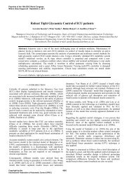
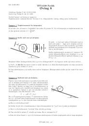
esented as a lumped parameter Quarter of Vehicle (QoV)
model illustrated on figure 1. It consists of the sprung mass
Fig. 1.
Quarter of vehicle
ms
k s MR
m us
m s (weight of cabin, power engine, etc), unsprung mass m us
(weight of tire, wheel, arms), the suspension strut and the
stiffness of the tire k t . A suspension strut is composed of
a spring k s , a passive damping element c p , and a variable
damping c v . The road disturbances, z r , excites the QoV
model. The vertical displacements of sprung, and unsprung
masses, z s and z us , result from the ground excitation.
Finally, the dynamic behavior of a Quarter of Vehicle
with a semi-active suspension is described by the following
system of ordinary differential equations:
kt
F
m s¨z s = −F MR − k s z def
m us¨z us = k s z def + F MR − k t (z us − z r )
where m s and m us are the sprung and unsprung mass,
respectively; z def is the suspension deflection; z r represents
the road profile; k s and k t are respectively the stiffness of
the suspension and the tire and F MR the semiactive damping
force.
The semi-active suspension is represented by an MRdamper,
which can be modeled as the sum of various
forces: a linear viscous friction (F c ), a spring force (F k )
and an electrically variable force (F I ) which is subject to
saturations. Thus, the resulting model for the damper force
(F M ) can be stated as:
F M = F I + F c + F k
F M = If c tanh(a 1 ż def + a 2 z def ) + b 1 ż def + b 2 z def (2)
} {{ } } {{ } } {{ }
F I
F c F k
which can be rewritten:
z
z
s
z r
us
(1)
F M = If c ρ 1 + b 1 ż def + b 2 z def (3)
where ρ 1 = tanh(a 1 ż def + a 2 z def ). The parameters f c ,
ρ 1 , a 1 , a 2 , b 1 and b 2 characterize the magneto-rheological
damper and has been obtained thanks to experimental results
[32]. Its value are :
Variable Description Value
I Electric current [A]
f c Dynamic yield force in the
MR damper model
600.95
[N.A −1 ]
ρ 1 Varying parameter to represent
hysteresis of the
damper
a 1 Pre-yield viscous damping
coefficient in MR damper
37.85
[N.m −1 ]
a 2 Pre-yield viscous damping
coefficient in MR damper
22.15
[N.m −1 ]
Post-yield viscous damping 2,830.86
b 1
b 2
coefficient in MR damper
Post-yield viscous damping
coefficient in MR damper
[N.s.m −1 ]
-7,897.21
[N.s.m −1 ]
In the study, each corner of the vehicle is equipped with 3
sensors: chassis acceleration ¨z s , wheel acceleration ¨z us and
a deflection sensor z def . However, the chassis acceleration
sensor ¨z us is faulty. The fault is considered to be additive.
In effect, most of accelerometers are subject to biases which
can be represented by an additive fault. The dynamical model
given in (1) is completed with the dynamics of the damper
(3). It results a state-space representation of the QoV model
as :
⎡
⎤ ⎡
¨z s
⎢ ż s
⎥
⎣¨z us
⎦ = ⎢
⎣
ż us
} {{ }
ẋ
− b1
m s
− c1 b 1 c 1
⎤ ⎡ ⎤
m s m s m s
ż s
1 0 0 0
⎥ ⎢ z s
⎥
b 1 c 1
m us m us
− b1
m us
− c1+kt ⎦ ⎣ż m us
⎦
us
0 0 1 0 z us
} {{ } } {{ }
⎡
− fcρ1
m s
0
f cρ 1
m us
⎤
A
⎡
− 1 m s
⎤
0
+ ⎢ ⎥
⎣ ⎦ I + ⎢ 0
⎥
⎣ 1 ⎦ F o + ⎢
0
⎥
⎣ k t ⎦ z r (4a)
m us
m us
0
0
0
} {{ } } {{ } } {{ }
B I B F B r
where the measurement vector y provided by the 2 accelerometers
¨z s , ¨z us and the deflection sensor z def is given
by :
⎡ ⎤
¨z s
y = ⎣ ¨z us
⎦
z def
⎡ ⎤
⎡
− b1
m s
− c1 b 1 c 1
⎤ ż s
m s m s m s
= ⎣ b 1 c 1
m us m us
− b1
m us
− c1+kt ⎦ ⎢ z s
⎥
m us ⎣ż us
⎦
0 1 0 −1
} {{ } z us
C
⎡ ⎤ ⎡ ⎤ ⎡ ⎤
− fcρ1
m s
0 1
+ ⎣ f cρ 1 ⎦ I + ⎣ k t ⎦
m us
m us
z r + ⎣0⎦
F o (4b)
0 0 0
} {{ } } {{ } }{{}
D I D r D F
with c 1 = k s + b 2 .
In this model, non linearity of the MR-damper ρ 1 appear
in a linear way in the matrices B I and D I of the system,
⎡
⎤
x
3804

so the system is LPV. Moreover, the system is subject to the
road excitation z r which is considered as a disturbance for
control and fault estimation. The control input of the system
is the electric current I inside the MR-damper.
B. Analysis of control laws
The QoV model suspension tuning looks for good comfort,
road holding and safe suspension deflections, [26]:
• The vertical chassis acceleration (¨z s ) response to road
disturbances (z r ), between 0 and 20 Hz, represents
the felt acceleration by the driver, i.e. ride comfort
specification.
• The vertical wheel deflection (z us −z r ) response to road
disturbances (z r ), between 0 and 30 Hz represents the
ability of the wheel to stay in contact with the road, i.e.
the road-holding specification.
For road holding the hard damping suspension is desirable,
but it deteriorates the ride comfort. The performance will be
obtained through of the control system focused on comfort
and road holding. Hence the goals of the control system are:
(1) the minimization of the vertical acceleration (¨z s ) gain in
the frequency of resonance of the sprung mass, and (2) the
minimization of the tire deflection (z us -z r ), in the frequency
of resonance of the tire deflection
III. FAULT ESTIMATION
The objective of the fault estimation is to estimate the fault
F o in the sensor. The proposed method is based on the H ∞
theory. Since the classical H ∞ approach is generally used
for controller synthesis, it can be easily extended for fault
detection and estimation. The objective of the synthesis is to
minimize the error of estimation between the fault and its
estimation, Fig. 2.
f 0
˜f
W W
u I
O
G s
ˆf
Fig. 3.
Standard
Controller [ ]
Kc
K s =
K d
Standard
Plant P
[ ] y
u
Problem under standard form
These “weighting filters” W I and W O allow us to specify
the frequency behavior of the closed loop system.
According to the scheme in Fig. 2, the fault estimation
error is given by :
˜f f − ˆf
[ y
= T F o − K e
u
= T F o − K e1 y − K e2 u
]
= T F o − K e2 u − K e1 G QoV u − K e1 G f F o
= (T − K e1 G f )F o − (K e2 + K e1 G QoV )u (5)
It can be shown that the fault estimation is directly affected
by both the fault itself F o and also the control input u.
A good estimation is achieved when the fault error ˜f is
as small as possible. In order to achieve this objective, a
weighting filter W f W f as illustrated in Fig. 4 is introduced
in the output ˜f.
20
Sensitivity of the estimation error
z
S f
0
W f
u
QoV System
y
Singular Values (dB)
−20
−40
−60
−80
f o
G(s)
−100
H ∞ Fault
Estimator
Fig. 2.
Matching
Filter
T
f
ˆf
+
-
Fault estimation problem
The optimization problem is rewritten in the “standard
form” problem, Fig. 3, where it is added “weighting filters”
W I and W O .
˜f
−120
10 −2 10 0 10 2 10 4
Frequency (rad/s)
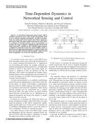
Fig. 4. Sensitivity of the estimation error S f and its corresponding
sensitivity filter W f
Its strong attenuation in low frequencies permits to have
a low estimation error ˜f, and so a good fault estimation. On
the other hand, the reader can easily appreciate the interest of
the matching filter T since it allows to specify the frequency
specification of the fault estimation.
Remark 1: In the structure of the fault estimator, it has
been chosen to consider as inputs both : 1 - the output of
3805

Semi-active suspension system based on
independent QoV control system
K
k t
m
m
s
2 Zones
MR damper
Model
us
I
z..
s
.
zs
Threshold
..
z us
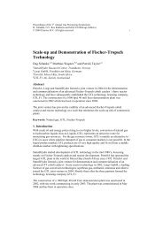
Fig. 5. F-Class vehicle and the semi-active suspension control system
based on a QoV model.
the system y and 2 - the control input u. This second input
is not mandatory/classical for the purpose of fault detection.
However, is presence is clearly justified in this purpose as it
brings a second degree of freedom K e2 appreciated in the
right and side of equation (5).
IV. ADD CONTROLLER
Model-free controllers are the most used in commercial
vehicles; examples of this approach are ground-hook, modified
sky-hook and the mix-1-sensor [28], [23], [27]. Because
of that, a model-free controller based on the On-Off Semi-
Active OSA control scheme is proposed.
The Acceleration Driven Damping (ADD) was developed
in [30], and [31]. It uses the the signs of the body vertical
acceleration ¨z s and the suspension relative velocity (ż s −ż us )
to select between the minimum and maximum damping
coefficients each sampling time. The main goal for this
control approach is to minimize the vertical acceleration. The
control law of the ADD controller is given by the equation
6.
c in (t) = c max if ¨z s (ż s − ż us ) ≥ 0
(6)
c in (t) = c min if ¨z s (ż s − ż us ) < 0
The ADD performance was studied in [30]. It was demonstrated
that the controller has significant benefits at bandwidths
beyond the sprung mass resonance frequency, but near
this the controller behaves similar to a passive suspension.
For this work, in particular, the ADD control scheme was
selected because its dependance of the vertical acceleration.
This because it uses directly the measured vertical acceleration
to compute the control law and a fail in its measure
impacts strongly on the decision of the damping coefficient.
A. Presentation and Scenario
V. APPLICATION
A F-Class vehicle, is a luxury car highly equipped, with
excellent performance in handling and comfort, detailed
construction, and innovative technology. Specifically for this
work, the car selected posses an independent suspension
configuration in each corner, where each one uses an MR
damper, and a deflection sensor.
The MR damper receives the electric current generated
by the ADD controller, Fig.5. The MR damper model, used
.
zus
z r
FDI
ADD
in simulations is two 2-Zones model, which is a modified
version of model in [25], simulates the MR damper force in
pre-yield and post-yield zones, the gain of damping force due
to electric current is independent of the velocity of piston:
⎧
⎨
F D =
⎩
c p ż + k p z + c MRpre−yield Iż
c p ż + k p z + c MRpost−yield I ż
|ż|
for |ż| < v yield
for |ż| > v yield
(7)
where F D is MR-damping force, k p is the stiffness coefficient,
c p is the damping coefficient, c MRpost−yield is the
damping coefficient in post-yield zone due to electric current,
c MRpreyield is the joint damping coefficient due to electric
current and velocity of piston in pre-yield, and v yield is
the velocity where the MR damping force yields and the
fluid changes from viscous to non Newtonian. The model
has a precision of 2 % when it simulates a random piston
displacement, [21], under persistent electric current.
The full vehicle simulation was made using CarSim TM .
The axis system is the vehicle-body-fixed system, SAE
standard J670e, [22].
The test was implemented in CarSim TM to evaluate the full
vehicle model, Fig. 6. The test was a Random road profile.
This profile tests the suspension under typical operation
conditions, Fig 6.
Roughness [m]
0.005
0
−0.005
(a) RP roughness
(b) CarSim
Fig. 6.
0 50 100
TM
Longitud [m]
simulation
Implemented test in CarSim TM for full vehicle.
The lumped parameters of front and rear QoV models are
needed for the controller design. These are obtained from
the vehicle parameters, Table I.
Thus, the sprung mass corresponding to the front left
corner, comprises the vehicle chassis and components. This
mass is supported by the suspension. The unsprung mass
corresponds to the wheel components, links and tire. Both
3806

TABLE I
PARAMETERS OF A F-CLASS VEHICLE IN CARSIM TM MODEL.
0.6
Roll : Comparison of the different controls
Variable Description Value Unit
m sfront Front QoV sprung mass 546.5 Kg
m us QoV unsprung mass 50 kg
k sf Front spring stiffness 83 N/mm
k t All tire stiffness 230 N/mm
(m us ), and (m s ) are obtained from the full vehicle parameters.
The lumped parameters of the QoV model follows a
distribution of the body weight of 60 % in front and 40 %
rear. Hence, a single front corner of the vehicle has a 30 %
of the total body weight.
B. Results
It is added an additive fault F o on the sprung mass
accelerometer :
¨z s = ¨z s,acc + F o
The fault of F o = +10m.s −2 arrives at time t = 10s.
Figure 7 shows the performance of the H ∞ fault estimator.
Roll [deg]
0.4
0.2
0
−0.2
−0.4
−0.6
Fault tolerant Control
−0.8
0 2 4 6 8 10 12 14 16 18 20
Time [s]
0.2
0.15
Fig. 8.
Faulty control
Comparison of the roll
Vertical acceleration : Comparison of the different controls
Faulty control
Fault tolerant Control
Estimated fault [m.s −2 ]
12
10
8
6
4
2
Estimated fault
Vertical acceleration [m.s −2 ]
0.1
0.05
0
−0.05
−0.1
−0.15
−0.2
0 2 4 6 8 10 12 14 16 18 20
Time [s]
0
−2
0 5 10 15 20 25
Time [s]
Fig. 9.
Comparison of the vertical acceleration
Fig. 7.
Estimated fault
A reconfiguration mechanism has been also considered in
this study. It consists of a simple switch. In fault free case,
the semi-active control allows to increase the comfort of the
passengers. When a fault is detected, the semi-active control
is no more used, and a passive suspension is considered :
{
IADD in fault free case
I =
if there is a fault
I 0
where I 0 represents the nominal value of the current.
In effect, when the fault occurs the control strategy if degraded
since its computation is based on the measurements.
The following figures show the roll (Fig. 8) and vertical
acceleration (Fig. 9) of the vehicle. The classical ADD
controller (solid blue lines) show that the performances of the
controller are degraded in the presence of the fault (t ≥ 10s).
Nevertheless, red dashed lines show the response of the
accommodated Controller. When a fault is detected, the
controller output is kept constant to a nominal value in order
to achieve performances of a passive damper. Thanks to this
approach, the performances are not so degraded.
VI. CONCLUSION
A robust Fault-Tolerant methodology for semi-active suspension
control is presented in this paper. The innovation
in this paper relies in the combination of an approved
control law (namely ADD) and a Fault detection approach.
In this paper, the fault detector is made from the H ∞
background. The interest of this approach relies in the robust
design. On the other hand, the ADD controller presents good
performances for comfort. However, this paper highlight the
effect of a sensor fault on the system. In effect, it is shown
that the performances of the ADD controller are degraded
when a fault occurs. The fault accommodation controller
switch to a passive damper when a fault is detected. This
3807

control strategy allows to reduce the bad performances due
to the fault.
REFERENCES
[1] R.J. Patton, “Fault Tolerant Control: The 1997 Situation”, 3 rd IFAC
SAFEPROCESS, England, August 1997, pp. 1033-1055.
[2] Y. Zhang and J. Jiang, “Bibliographical Review on Reconfigurable
Fault-tolerant Control Systems”, Annual Reviews in Control, vol. 32,
2008, pp. 229-252.
[3] E. Chow and A. Willsky, “Analytical Redundancy and the Design
of Robust Failure Detection Systems”, IEEE Trans. on Automatic
Control, vol. 1, 1984, pp. 603-619.
[4] R.J. Patton and J. Chen, “A Review of Parity Space Approaches to
Fault Diagnosis for Aerospace Systems”, J. of Guidance, Control and
Dynamics, vol. 17(2), 1994, pp. 278-285.
[5] J. Gertler, “Fault Detection and Isolation Using Parity Relations”,
Control Eng. Practice, vol. 5(5), 1997, pp. 653-661.
[6] Basseville, M. and Nikiforov, I.V., “Detection of Abrupt Changes -
Theory and Application”, Prentice- Hall, Inc., Englewood Cliffs, N.J.,
1993
[7] Balas, G. and Bokor, J., and Szabo Z. “Invariant subspace for lpv
systems and their applications”, IEEE Transactions on Automatic
Control, 2003, vol. 48, pp. 2065–2069.
[8] Ding, S. “Model-based Fault Diagnosis Techniques”, Springer, Berlin,
2008.
[9] P. Apkarian, P. Gahinet and G. Becker, “Self-scheduled H ∞ Control of
Linear Parameter-Varying Sistems: A Design Example”, Automatica,
vol. 31, 1995, pp. 1251-1261.
[10] C. Sloth, T. Esbensen and J. Stoustrup, “Active and Pasive Fault-
Tolerant LPV Control of Wind Turbines”, American Control Conf.,
USA, Jun-Jul 2010, pp. 4640-4646.
[11] M. Rodrigues, D. Theilliol, S. Aberkane and D. Sauter, “Fault Tolerant
Control Design for Polytopic LPV Systems”, Int. J. AMCS, vol. 17(1),
2007, pp. 27-37.
[12] A. Vargas-Martínez, V. Puig, L.E. Garza-Castañón and R. Morales-
Menendez, “MRAC + H ∞ Fault Tolerant Control for Linear Parameter
Varying Systems”, SysTol’10, France, Oct. 2010, pp. 94-99.
[13] A. Chamseddine and H. Noura, “Control and Sensor Fault Tolerance
of Vehicle Active Suspension”, IEEE Trans. on Control Systems Tech.,
vol. 16(3), 2008, pp. 416-433.
[14] P. Gáspár, Z. Szabó and J. Bokor, “LPV Design of Fault-tolerant
Control for Road Vehicles”, SysTol’10, France, Oct. 2010, pp. 807-
812.
[15] D. Fischer and R. Isermann, “Mechatronic Semi-active and Active
Vehicle Suspensions”, Control Engineering Practice, vol. 12, 2004,
pp. 1353-1367.
[16] S. Guo, S. Yang and C. Pan, “Dynamical Modeling of Magnetorheological
Damper Behaviors”, J. of Intell. Mater., Syst. and Struct.,
vol. 17, 2006, pp. 3-14
[17] C. Poussot-Vassal, O. Sename, L. Dugard, P. Gáspár, Z. Szabó and J.
Bokor, “A New Semi-active Suspension Control Strategy through LPV
Technique”, Control Eng. Practice, vol. 16, 2008, pp. 1519-1534.
[18] A.L. Do, O. Sename and L. Dugard, “An LPV Control Approach for
Semi-Active Suspension Control with Actuator Constraints”, American
Control Conf., USA, Ju.-Jul. 2010, pp. 4653-4658.
[19] S. Varrier, D. Koenig and J.J. Martinez, “A Parity Space-Based Fault
Detection On LPV Systems : Approach For Vehicle Lateral Dynamics
Control System”, 8 th IFAC SAFEPROCESS, Mexico, 2012.
[20] S. Varrier, D.Koenig and J.J. Martinez, “Robust Fault Detection
for Vehicle Lateral Dynamics”, IEEE Conference on Decision and
Control, Hawai, 2012.
[21] C. Boggs and L. Borg and J. Ostanek, “Efficient Test Procedures
for Characterizing MR Dampers”, ASME 2006 Int. Mechanical Eng
Congress and Exposition, 2006.
[22] T. D. Gillespie, “Fundamentals of Vehicle Dynamics”, SAE Int, 1992.
[23] K. S. Hong and H. C. Sohn and J. K. Hedrick, “Modified Skyhook
Control of Semi-Active Suspensions: A New Model, Gain Scheduling,
and Hardware-in-the-Loop Tuning”, J. Dyn. Sys., Meas., Control,
March 2002, pp 158–167.
[24] J. Lozoya-Santos and R. Morales-Menendez and O.Sename and R.
Ramirez and L. Dugard, “Control Strategies for an Automotive Suspension
with a MR Damper”, IFAC World Conf, 2011
[25] D. Maher and P. Young, “An Insight into Linear Quarter Model
Accuracy”, Vehicle Syst. Dyn., 2011, vol. 49, pp. 463–480
[26] C. Poussot-Vassal and C. Spelta and O. Sename and S.M. Savaresi and
L. Dugard, “Survey and Performance Evaluation on Some Automotive
Semi-Active Suspension Control Methods: A Comparative Study on a
Single-Corner Model”, Annual Reviews in Control, 2012, vol. 36, pp.
148–160
[27] S. M. Savaresi and C. Spelta, “A Single-Sensor Control Strategy
for Semi-Active Suspensions”, Control Systems Technology, IEEE
Transactions on, 2009, vol. 17, pp. 143–152
[28] M. Valasek and M. Novak and Z. Sika and O. Vaculin, “Extended
Ground-Hook – New Concept of Semi-Active Control of Truck
Suspension”, Vehicle Syst. Dyn., 1997, vol. 29, pp. 289–303
[29] Robert, D. “Contribution linteraction commande/ordonnancement”
Ph.D. thesis, Institut National Polytechnique de Grenoble, 2007
[30] S. M. Savaresi and E. Silani and S. Brittanti, “Acceleration-Driven-
Damper (ADD): An Optimal Control Algorithm for Comfort-Oriented
Semi-Active Suspensions”, ASME J. Dyn. Syst., Meas., Control, 2005,
vol. 129(2), pp. 218–229
[31] S. M. Savaresi and E. Silani and S. Brittanti and N. Porciani, “On
Performance Evaluation Methods and Control Strategies for Semi-
Active Suspension Systems”, 42nd Control and Decision Conference,
2003, pp. 2264–2269
[32] J.-d.-J. Lozoya-S., R. Morales-M., R. Ramirez-M., J.-C. Tudón-M., O.
Sename, L. Dugard, “Magneto-Rheological damper - an experimental
study”, Journal of Intelligent Material Systems and Structures 23, 11
(2012), pp. 1213–1232
3808