Turbulence Modelling– 2 - Turbulence Mechanics/CFD Group

School of Mechanical Aerospace and Civil Engineering 

Turbulence Modelling– 2 

T. J. Craft 

George Begg Building, C41 

3rd Year Fluid Mechanics 

Contents: 

Reading: 

◮ Navier-Stokes equations 

F.M. White, Fluid Mechanics 

◮ Inviscid flows 

J. Mathieu, J. Scott, An Introduction to Turbulent Flow 

◮ Boundary layers 

P.A. Libby, Introduction to Turbulence 

◮ Transition, Reynolds averaging 

P. Bernard, J. Wallace, Turbulent Flow: Analysis Mea- 

◮ Mixing-length models of turbulence 

surement & Prediction 

◮ S.B. Pope, Turbulent Flows 

Turbulent kinetic energy equation 

◮ 

D. Wilcox, Turbulence Modelling for CFD 

One- and Two-equation models 

◮ 

Notes: http://cfd.mace.manchester.ac.uk/tmcfd 

Flow management 

- People - T. Craft - Online Teaching Material 

◮ As before, we can prescribe a lengthscale, and take ε as k 3/2 /l. The only 

unknown quantity in equation (2) is then the diffusion of k. 

◮ The molecular diffusion of k does not need modelling – but it is usually 

negligible compared with the turbulent contribution, except in the viscous 

sublayer. 

◮ The turbulent diffusion of k is usually modelled as a gradient transport 

process, giving: 

 

∂ 

Diffk = ν + 

∂y 

νt 

 

∂k 

σk ∂y 

(3) 

where σ k is known as the turbulent Prandtl number for the diffusion of 

kinetic energy, usually taken as unity. 

◮ Thus, with the above one-equation model, l is prescribed algebraically, 

and k is found as the solution of the transport equation 

 

Dk ∂ 

= ν + 

Dt ∂y 

νt 

 

∂k k 

+ Pk − 

σk ∂y 

3/2 

(4) 

l 

Turbulence Modelling– 2 2010/11 3 / 19 

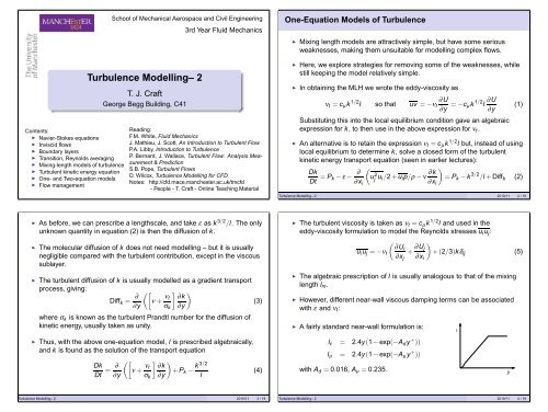
One-Equation Models of Turbulence 

◮ Mixing length models are attractively simple, but have some serious 

weaknesses, making them unsuitable for modelling complex flows. 

◮ Here, we explore strategies for removing some of the weaknesses, while 

still keeping the model relatively simple. 

◮ In obtaining the MLH we wrote the eddy-viscosity as 

νt = cμk 1/2 ∂U 

l so that uv = −νt 

∂y = −cμk 1/2 l ∂U 

∂y 

Substituting this into the local equilibrium condition gave an algebraic 

expression for k, to then use in the above expression for νt. 

◮ An alternative is to retain the expression νt = cμk 1/2 l but, instead of using 

local equilibrium to determine k, solve a closed form of the turbulent 

kinetic energy transport equation (seen in earlier lectures): 

Dk 

Dt = P k − ε − ∂ 

∂x i 

 

u 2 j u i/2+u ip/ρ − ν ∂k 

∂x i 

(1) 

 

= P k − k 3/2 /l + Diffk (2) 


◮ The turbulent viscosity is taken as νt = cμk 1/2l and used in the 

eddy-viscosity formulation to model the Reynolds stresses uiuj: 

∂Ui 

uiuj = −νt + 

∂xj ∂U 

j 

+(2/3)kδ ij 

∂xi ◮ The algebraic prescription of l is usually analogous to that of the mixing 

length lm. 

◮ However, different near-wall viscous damping terms can be associated 

with ε and νt: 

◮ A fairly standard near-wall formulation is: 

lε = 2.4y(1 − exp(−Ady + )) 

lμ = 2.4y(1 − exp(−Aμy + )) 

with A d = 0.016, Aμ = 0.235. y 


l 

(5)

◮ One advantage of solving an equation for k 

is that the turbulence energy, and thus the 

viscosity, does not now have to vanish 

when ∂U/∂y vanishes locally. 

◮ In the wall-jet example shown, P k is non-zero either side of the velocity 

maximum. Although it will be zero at the peak, k will be non-zero, being 

diffused across this region. 

◮ Some transport effects have thus been incorporated into the turbulence 

model. 


Two-Equation Models 

◮ In complex flows, prescribing the lengthscale becomes impossible. It may 

be difficult to define the distance to the wall, and the local level of l is 

affected by convection and diffusion processes. 

bl thicker on upper 

surface due to apg 

y 

x 

larger lengthscale 

due to thickening bl 

◮ An alternative, building on the modelling already y adopted for k, is to 

y 

obtain l from its own separate transport equation. 

l 

l 

more uniform 

lengthscale 

further 

downstream 

◮ Most two-equation models solve a transport equation for a variable of the 

form k 

U 

U 

al b . Since we also solve the k transport equation, this enables us 

to obtain l. 

◮ A popular choice of second variable is ε, the dissipation rate of k. ie 

a = 3/2, b = −1 (since ε = k 3/2 /l). 


Other One-Equation Models 

◮ Although we have considered a transport equation for k, other 

one-equation models have been proposed, where the transport equation 

is for some other variable. 

◮ Amongst others, Barth (1990), Spalart & Allmaras (1994) and 

Menter (1994) have all developed models that solve for νt itself. 

◮ A typical example is that of Menter (1994): 

 

∂Ui 

Dνt 

= c1νt − 

Dt ∂xj ∂Uj 

2 ν 

− c2 

∂xi 2 

t ∂ νt ∂νt 

+ 

l2 ∂xj σν ∂xj ◮ Different one-equation models will perform somewhat differently in 

particular flows, but are generally more widely applicable than 

mixing-length schemes. 

◮ However, they do still need a lengthscale to be prescribed – in the above 

example for the destruction term in the νt transport equation. 


The k-ε Model 

◮ In earlier lectures we obtained a transport equation for k. 

◮ It is possible to derive an exact transport equation for ε, by manipulating 

the transport equations for u i (since ε = ν(∂ui/∂xj) 2 ). 

◮ However, the result is not very useful for direct modelling purposes: most 

of the terms appearing in it need to be modelled. A modelled transport 

equation for ε is thus usually devised via a more empirical approach. 

◮ Typical model ε equations are devised by reference to the k equation: 

Dε 

Dt 

= 

ε 

cε1 

k Pk 

Source 

− 

ε 

cε2 

2 

 

k 

 

Sink 

+ 

 

∂ 

ν + 

∂xj νt 

 

∂ε 

σε ∂xj 

Diffusion 

(7) 

◮ The source term ensures that if k is being created by mean shear the 

dissipation rate also increases. 

◮ The sink term ensures that if P k is zero both k and ε decrease. 


(6)

◮ The turbulent timescale k/ε and model coefficients cε1 and cε2 are 

associated with the generation and destruction terms. 

◮ The simple diffusion model is similar to that adopted in the k equation. 

◮ The coefficients cε1, cε2 and σε are taken as constants, to be tuned over 

a range of flows. 

◮ Generally, one might expect that the wider the range of flows considered 

when tuning these model coefficients, the more applicable the scheme 

will be to complex, real-life, flow situations. 

◮ We now consider how values for these model coefficients are typically 

obtained. 


◮ Equation (8) gives an expression for ε. Substituting this, and the 

expression for k, into equation (9) leads to: 

−U 2 cn(n+1)x −(n+2) c 

= −cε2 

2n2U 2x −2(n+1) 

cx −n 

◮ Cancelling common factors gives 

(n+1) = ncε2 or cε2 = n+1 

n 

◮ From experiments, the decay rate n ≈ 1.1, giving cε2 ≈ 1.9. 

◮ Thus, taking cε2 ≈ 1.9 in the model should ensure that it will return the 

correct rate of decay of turbulence in the absence of any generation. 


(10) 

Decaying Grid Turbulence 

◮ A value for cε2 can be found by considering decaying grid turbulence. 

◮ In a uniform stream passed2 through a 

turbulence-generating grid, 1k 

decays x 

downstream of the grid (there are no 

x 

velocity gradients, so Pk = 0). 

3 

◮ k decays exponentially with distance downstream of the grid, k = cx 

) 

−n . 

The constants c and n can be measured experimentally. 

2 

y 

◮ In such decaying homogeneous 1 grid turbulence, Pk = 0 and diffusion can 

be neglected. 

◮ The k and ε equations then reduce to 

U dk 

dx 

U dε 

dx 

2 

d 

= −ε or ε = −U 

3 dx (cx −n ) = cnUx −(n+1) 

ε 

= −cε2 

2 

k 


Log-Law Region of an Equilibrium Boundary Layer 

y 

U 

k 

k=cx −n 

◮ In an earlier lecture we saw that in the fully turbulent, local equilibrium, 

region of a simple boundary layer we should have: 

2 

Pk = ε |uv | = uτ |uv |/k = c 1/2 

μ so k = u 2 τ /c 1/2 

μ 

where the friction velocity uτ ≡ (τw/ρ) 1/2 . 

◮ The mean velocity satisfied the log-law: 

U 

uτ 

= 1 

log(Eyuτ/ν) so 

κ 

∂U uτ 

= 

∂y κy 

and νt = κyuτ 

◮ As a second constraint we ensure that the modelled ε equation will return 

the above results in a simple boundary layer. 

◮ The convection term Dε/Dt can be neglected, but diffusion cannot be 

ignored (the lengthscale increases linearly with wall-distance, so 

ε = k 3/2 /(2.5y) and hence ε ∝ 1/y). 


x 

(8) 

(9)

◮ The ε transport equation in this case then becomes 

 

νt 

0 = P2 k 

d 

(cε1 − cε2)+ 

k dy 

= (uv )2 

k 

σε 

d(P k) 

dy 

2 ∂U 

(cε1 − cε2)+ 

∂y 

d 

dy 

 

νt d 

−uv 

σε dy 

∂U 

 

∂y 

◮ Substituting in the earlier expressions for uv , k, ∂U/∂y and νt then gives 

0 = u 4 u 

τ 

2 τ 

κ2y 2 

c 1/2 

μ 

u2 (cε1 − cε2)+ 

τ 

d 

 

κyuτ d 

u 

dy σε dy 

2 

uτ 

τ 

κy 

= u4 τ c1/2 μ 

κ2 

d u4 τ y 1 

(cε1 − cε2) − 

y 2 dy σε y 2 

 

= u4 τ c 1/2 

μ 

κ2y 2 (cε1 − cε2)+ u4 τ 

σεy 2 

◮ Cancelling u4 τ /y 2 leaves a relation between the model coefficients cε1, 

cε2, and σε: 

c 1/2 

μ (cε1 − cε2) 

κ2 = − 1 

σε 

(11) 


The Resultant k-ε Model 

◮ A commonly used set of coefficients, obtained as outlined above, is 

cμ σ k σε cε1 cε2 

0.09 1.0 1.3 1.44 1.92 

◮ In summary, the k-ε model then solves transport equations for k and ε: 

Dk 

Dt = Pk − ε + ∂ 

Dε 

Dt 

= 

 

νt ∂k 

∂xj σk ∂xj εPk ε 

cε1 − cε2 

k 

(12) 

2 

∂ νt ∂ε 

+ 

k ∂xj σε ∂xj 

(13) 

and uses the linear stress-strain relation: 

 

∂Ui 

uiuj = (2/3)kδij − νt + 

∂xj ∂U 

j 

∂xi with turbulent viscosity νt = cμk 2 /ε. 


(14) 

◮ We thus want to choose model coefficients that satisfy equation (11), to 

ensure the model will return an appropriate logarithmic velocity profile 

when applied to a local equilibrium boundary layer. 

◮ The model will then return a lengthscale k 3/2 /ε that does increase 

linearly with wall distance in a local equilibrium boundary layer. 

◮ However, in more complex flows it need not always return this same 

variation (whereas in the simpler models considered, we imposed such a 

variation regardless of local flow conditions). 

◮ To finally determine the coefficients, cε1 is chosen from computer 

optimization, considering simple free flows (eg. plane jet or mixing layer). 


◮ The k-ε model is generally more expensive to apply than zero- or 

one-equation schemes. 

◮ On the other hand, it does not require one to prescribe lengthscales 

across the flow, and is thus more convenient to apply to complex flow 

geometries. Only appropriate boundary conditions for k and ε need to be 

provided at the flow domain edges. 

◮ Wall-jet profiles show better performance than the one-equation model 

results seen earlier. 

Turbulence Modelling– 2 2010/11 16 / 19

Other Two-Equation Models 

◮ Other two-equation models mostly still solve a transport equation for k, 

but use the second equation to solve for something other than ε. 

◮ For example, the k-ω model of Wilcox (1988) solves for ω (≡ ε/k): 

Dk 

Dt = P k − ωk + diffusion (15) 

Dω ωPk = cω1 

Dt k − cω2ω2 + diffusion (16) 

and defines the turbulent viscosity as νt = cμk/ω. 

◮ The model coefficients in these other schemes are usually obtained in 

similar ways to those already outlined for the ε equation. 

◮ In the near-wall, viscosity-affected, layer most two-equation models 

include a number of ‘damping’ terms – usually dependent on either the 

turbulent Reynolds number (Rt = k 2 /(εν)) or non-dimensional wall 

distance y + . Details of these are not considered here. 


◮ There are a number of more advanced modelling practices. 

◮ These range from simple refinements to coefficients, or more complex 

algebraic stress-strain relationships, through to full second-moment 

closures where separate transport equations are solved for each of the 

Reynolds stress components, u iuj. 

◮ A number of the more advanced schemes are now available in 

commercial CFD packages, but details of their development is beyond 

this course. 


Summary of Two-Equation Model Performance 

◮ For industrial engineering simulations, two-equation models are the most 

widely used approach for modelling the effects of turbulence. 

◮ The simpler modelling schemes often require substantial ad-hoc, 

case-by-case input to the model (eg. prescription of lengthscales). 

◮ Although not considered here, even two-equation models have a number 

of well-known weaknesses when applied to certain important classes of 

flows (eg. impinging flows, curved flows, rotating flows, . . . ). 

x 

r 

Q 

Turbulence Modelling– 2 2010/11 18 / 19

Turbulence Modelling– 2 - Turbulence Mechanics/CFD Group

You also want an ePaper? Increase the reach of your titles

Delete template?

Save as template?