Turbulent Heat Flux Modelling - Turbulence Mechanics/CFD Group

School of Mechanical Aerospace and Civil Engineering 

Turbulent Heat Flux Modelling 

T. J. Craft 

George Begg Building, C41 

MSc Fluid Mechanics 

Contents: 

◮ Navier-Stokes equations 

◮ Inviscid flows 

◮ Creeping Flows 

Reading: 

◮ Boundary layers 

F.M. White, Fluid Mechanics 

◮ Transition, Reynolds averaging J. Mathieu, J. Scott, An Introduction to Turbulent Flow 

◮ Turbulent heat transport 

P.A. Libby, Introduction to Turbulence 

◮ Mixing-length models of turbulence 

P. Bernard, J. Wallace, Turbulent Flow: Analysis Mea- 

◮ Turbulent kinetic energy equation 

◮ Turbulent heat flux modelling 

◮ One- and Two-equation models 

◮ Flow management 

surement & Prediction 

S.B. Pope, Turbulent Flows 

D. Wilcox, Turbulence Modelling for CFD 

Notes: http://cfd.mace.manchester.ac.uk/tmcfd 

- People - T. Craft - Online Teaching Material 

Eddy-Diffusivity Models 

◮ When considering the dynamic field, an analogy was drawn between the 

Reynolds stresses and viscous stresses. 

◮ This led to the eddy-viscosity approach of modelling 

 

∂Ui 

uiuj = −νt + 

∂xj ∂U 

j 

+(2/3)kδ ij 

∂xi with νt being the eddy (or turbulent) viscosity. 

◮ We noted that νt is not a property of the fluid, but depends on local flow 

conditions. 

◮ Apart from in the viscous sublayer, νt is generally much larger than ν. 

◮ We examined a number of modelling approaches for approximating νt, 

ranging from mixing-length (zero-equation) schemes to two-equation 

models. 

Turbulent Heat Flux Modelling 2010/11 3 / 11 

(2) 

Introduction 

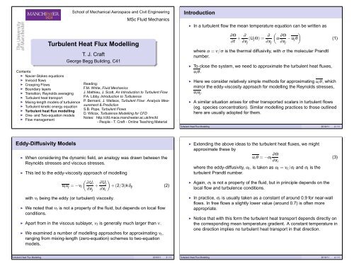
◮ In a turbulent flow the mean temperature equation can be written as 

 

∂Θ ∂ ∂ 

+ (U 

∂t ∂x 

jΘ) = α 

j ∂xj ∂Θ 

 

− u 

∂x 

jθ 

j 

where α = ν/σ is the thermal diffusivity, with σ the molecular Prandtl 

number. 

◮ To close the system, we need to approximate the turbulent heat fluxes, 

uiθ. 

◮ Here we consider relatively simple methods for approximating u iθ, which 

mirror the eddy-viscosity approach for modelling the Reynolds stresses, 

u iuj. 

◮ A similar situation arises for other transported scalars in turbulent flows 

(eg. species concentration). Similar modelling practices to those outlined 

here are usually adopted for them. 


◮ Extending the above ideas to the turbulent heat fluxes, we might 

approximate these by 

∂Θ 

uiθ = −αt 

∂xi 

where the eddy-diffusivity, αt, is taken as αt = νt/σt and σt is the 

turbulent Prandtl number. 

◮ Again, σt is not a property of the fluid, but in principle depends on the 

local flow and turbulence conditions. 

◮ In practice, σt is usually taken as a constant of around 0.9 for near-wall 

flows. In free flows a slightly lower value (around 0.7) is often more 

appropriate. 

◮ Notice that with this form the turbulent heat transport depends directly on 

the corresponding mean temperature gradient. A constant temperature in 

one direction implies no turbulent heat transport in that direction. 


(1) 

(3)

Turbulent Heat Fluxes in Simple Shear Flow 

◮ In a simple shear flow, with U(y), Θ(y), the eddy-diffusivity model gives 

uθ = −(νt/σt) ∂Θ 

= 0 

∂x 

vθ = −(νt/σt) ∂Θ 

U(y) 

∂y 

y 

x 

◮ In equilibrium conditions experiments suggest σt ≈ 0.7 − 0.8 and 

|uθ /vθ | ≈ 1.1 in an homogeneous free shear flow. 

◮ Measurements at 

higher strain rates 

show σt ≈ 1.1 and 

|uθ /vθ | ≈ 2.2. 


Buoyancy-Affected Flows 

◮ In a buoyancy-affected flow we saw an extra generation term appears in 

the k transport equation: 

G k = −β gi uiθ (5) 

◮ With the above eddy-diffusivity model we relate the turbulent heat fluxes 

directly to the corresponding temperature gradients. 

◮ To understand the model behaviour we thus examine two cases: one 

where the temperature gradient and gravitational vector are aligned, and 

one where they are not. 

U(y) 

g 

y 

x 

Θ(y) 

Tcold 


Thot 

g 

y 

x 

Θ(y) 

◮ Clearly the model prediction of uθ = 0 is not an accurate representation 

of reality. 

◮ However, if streamwise gradients are relatively small, misrepresenting uθ 

may not have too serious an effect, at least in some non-buoyant flows. 

◮ The reason for this can be seen from the 

boundary layer form of the mean 

temperature equation: 

U ∂Θ 

∂x 

∂Θ ∂ 

+ V = 

∂y ∂y 

 

α ∂Θ 

 

− vθ 

∂y 

(4) 

U(y) 

y 

x 

◮ In this situation only the cross-stream heat flux, vθ , is particularly 

influential. 


Horizontal Buoyant Flows 

◮ In the (stable) situation shown, using 

the eddy-diffusivity model for vθ , we 

now get 

G k = −β g vθ = β g(νt/σt) ∂Θ 

∂y 

U(y) 

y 

(6) x 

g 

Θ (y) 

Θ(y) 

◮ ∂Θ/∂y is positive, g is negative, so G k is negative as we would expect. 

◮ If the temperature gradient were reversed, G k would change sign, again 

as expected. 

◮ Although qualitatively showing the correct sign, such simple models are 

often not particularly accurate in a quantitative sense, particularly in 

stably stratified flows. 

Turbulent Heat Flux Modelling 2010/11 8 / 11

Vertical Buoyant Flows 

◮ Now consider a vertical flow as shown. 

◮ We still have 

G k = −β g vθ = β g(νt/σt) ∂Θ 

∂y 

(7) 

Thot 

g 

y 

x 

Tcold 

◮ However, ∂Θ/∂y is now rather small (the dominant temperature gradient 

is normal to the wall), so Gk is also small. 

◮ From the simple shear flow discussion earlier, we expect the model to 

underpredict the magnitude of the streamwise heat flux (vθ in this case). 

◮ Here, this underprediction can be expected to lead to an underestimation 

of the magnitude of G k. 


◮ If using the linear EVM formulation for the stresses the heat flux 

expressions become 

k 

uθ = cθ 

ε νt 

∂U ∂Θ 

∂y ∂y 

k 

vθ = −(2/3)cθ 

2 ∂Θ 

ε ∂y 

◮ The GGDH generally gives a better representation of the turbulent heat 

fluxes than the simple eddy-diffusivity model (in the above example, uθ is 

non-zero now). 

◮ However, to realize a significant improvement a better underlying model 

for the Reynolds stress components than the eddy-viscosity 

representation is often needed. 


The GGDH Heat Flux Model 

◮ An improved turbulent heat flux model is often provided by the 

generalized gradient diffusion model of Daly & Harlow (1970). 

◮ In this, we take 

k 

uiθ = −cθ 

ε u ∂Θ 

iuj ∂xj ◮ The constant cθ is typically taken around 0.3. 

◮ In a simple shear flow considered earlier, we now have 

k ∂Θ 

uθ = −cθ uv 

ε ∂y 

k ∂Θ 

y 

vθ = −cθ v 2 

ε ∂y x 

◮ Note that reliable values of the individual Reynolds stress components 

are now needed. 


U(y) 

Θ(y) 

(8)

Turbulent Heat Flux Modelling - Turbulence Mechanics/CFD Group

Create successful ePaper yourself

Delete template?

Save as template?