Buckling of thin-walled conical shells under uniform external pressure
Buckling of thin-walled conical shells under uniform external pressure
Buckling of thin-walled conical shells under uniform external pressure

You also want an ePaper? Increase the reach of your titles
YUMPU automatically turns print PDFs into web optimized ePapers that Google loves.
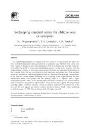
p cr p<br />
125<br />
120<br />
115<br />
110<br />
105<br />
By various substitutions [19], it can be shown that Eq. (1)<br />
can be transferred to the form<br />
0:92Eðte=RÞ 25<br />
pcr ¼ , (2)<br />
Le=R<br />
where te is the effective thickness <strong>of</strong> cone t cos a; t the<br />
thickness <strong>of</strong> cone; and Le the effective length <strong>of</strong> cone L/2<br />
(1+r/R). Thus, <strong>conical</strong> <strong>shells</strong> subjected to <strong>external</strong><br />
<strong>pressure</strong> may be analyzed as cylindrical <strong>shells</strong> with an<br />
effective thickness and length.<br />
6.1. Sole-fish buckling mode<br />
Fig. 8. Parametric considerations.<br />
100 0 0.1 0.2 0.3 0.4 0.5 0.6 0.7 0.8 0.9 1.0<br />
1-r/R<br />
Fig. 9. Cone function.<br />
An important parameter in buckling analysis <strong>of</strong> axisymmetrically<br />
loaded <strong>shells</strong>, for instance, the models thrashed<br />
out herein, is the number <strong>of</strong> circumferential waves in the<br />
buckling mode layout. Notionally speaking, the buckling<br />
mode is in the form <strong>of</strong> a single harmonic mode around the<br />
circumference, but in a test, owing to the incidence <strong>of</strong><br />
imperfections, miscellaneous modes may be implicated. A<br />
well-established way <strong>of</strong> construing geometric imperfection<br />
and deformation measurements to decipher the dominant<br />
harmonic modes and their relationship is to carry out<br />
ARTICLE IN PRESS<br />
B.S. Golzan, H. Showkati / Thin-Walled Structures 46 (2008) 516–529 525<br />
Fourier decompositions. Such decompositions were not<br />
carried out for the imperfection or deformation measurements<br />
on these models, since the form <strong>of</strong> buckling that was<br />
developed all over the cones was drastically outlying from a<br />
well-ordered wave configuration. On such specimens there<br />
was an overall buckling predisposed by position <strong>of</strong> weld<br />
lines and efficiency <strong>of</strong> the supports and formation <strong>of</strong> the<br />
initial leakage point. So as to set forth a better depiction <strong>of</strong><br />
this buckling, principally based on empirical remarks and<br />
for the first time we coined the name ‘‘sole-fish buckling<br />
mode’’ on this phenomenon. The spine <strong>of</strong> this animal can<br />
better illustrate the weld line and its impact on the other<br />
parts <strong>of</strong> the shell. The appearance <strong>of</strong> non-periodical waves<br />
can be easily spotted from this plot.<br />
7. Observations and milestones<br />
7.1. Frusta specimens<br />
In Figs. 10 and 11 a contrast is carried out between<br />
initial and ultimate geometry <strong>of</strong> specimen SC5 in which the<br />
maximum deformation is located roughly at the height<br />
<strong>of</strong> 1<br />
3 h.<br />
In all <strong>shells</strong> <strong>of</strong> this study the loading was continued to<br />
farther than the range <strong>of</strong> postbuckling behavior. It is<br />
observed that a ‘‘V’’ shape yield line is developed in the<br />
region close to the restrained boundaries <strong>of</strong> the frusta,<br />
before failure takes place. The same phenomenon was<br />
reported by Showkati [21]. InFig. 6 a typical behavior is<br />
represented for specimen SC5 and SC6.<br />
By escalating the <strong>external</strong> <strong>pressure</strong>, the failure mode<br />
was gradually approached. In most specimens, incidence<br />
<strong>of</strong> a very large displacement in one edge caused an<br />
288<br />
270<br />
252<br />
306<br />
234<br />
324<br />
216<br />
342<br />
198<br />
300<br />
280<br />
260<br />
240<br />
220<br />
200<br />
180<br />
160<br />
140<br />
120<br />
100<br />
80<br />
60<br />
40<br />
20<br />
0<br />
0<br />
180<br />
18<br />
162<br />
36<br />
144<br />
54<br />
126<br />
Fig. 10. Polar plot <strong>of</strong> final geometry measured on specimen SC5.<br />
72<br />
90<br />
108