Propagation Low-Frequency

More documents

Recommendations

Info

1962 Johler: Propagation of Low-Frequency Signal 413 where q5'=-45-7r/2=arg [E(co, d)] and E(co, d)= Eo(w, d).. The real part of the amplitude-time function (45) Re E(ti', d) is the desired function for the cosine source (41), and the imaginary part -Im E(t', d) = Re [iE(t', d) ] is the desired function for the sine source (42). This integral can be evaluated with the aid of quadrature techniques [23]. Thus, the problem has been reduced to the evaluation of a real integral rX E(t', d) = Ft(w, d)dw - Re f f(w, d) exp (iwt)dw. (46) _m The transfer function for the ground wave, E(Q, d), (38) which can now be inserted directly in the integrand of the Fourier integral is illustrated in Figs. 7 and 8. Since the transfer characteristic E(co, d) =Eo(w, d) is complex, both anmplitude and phase are presented as a function of frequency for various distances. The phase is presented as the phase lag ¢Ck where the total true phase arg [E(w, d) ] = - [kid +4c+r/2 ]. The effect of the conduction currents in the earth on the propagation has been introduced as the conductivity for typical land, a = 0.005 mho/m. The effect of the displacement currents in the earth on the propagation has been introduced by the dielectric constant E2 = 15 (relative to a vacuum). The permeability yLo=4ir(10-7) henry/meter has been assumed. The use of the series of residues applicable to propagation about a spherical earth takes account of the vertical lapse of the index of refraction of the earth's atmosphere [I] by the factor a (38) where a-0.75. Although it has been assumed that both transmitter and receiver are located on the surface of the earth, the effect of elevating transmitter and/or receiver can be introduced by multiplying each term of the series of residues (38) by the factorf8(h1)f8(h2) where hi and h2 are the height of the transmitter and receiver, respectively, above the surface of the earth, and (1), (13), (18) f8(h) = v 1 2 /3 - 2habl/3 - IV 2 (kia)213 - 2T IV2{ -(2)"1/3,r in which lv(z) is the modified Hankel function tabulated by Furry [24 ]. The integrand of the Fourier integral (Fig. 9) in the frequency-amplitude plane at some given local time t' can be related to the more conventional notion of the Fourier spectrum f(c(w, d) by eliminating the notion of a negative frequency w. Thus, the amplitude spectrum is I f2(w, d) I = I f(Co,d) + f(- , d)| (w > 0) (48) and the phase spectrum is 0.(w, d) = arg [f.(w, d)] = arg [f(w, d) + f(-w, d)] (w > 0). (49) The phase, cfr.(w, d) can be reckoned (Fig. 9) from the origin t' = 0 to the crest of the continuous wave or Fourier spectrum wave at a certain frequency (0.2 Mc, Fig. 9). The corresponding amplitude If(w, d) does not correspond to the amplitude of the integrand Fj(w, d). The two waves do intersect, however, at the point t'= 10 ,usec, (see, e.g., Fig. 9), at which point the Fourier spectrum wave enters the integration (45) with a phase shift beyond the crest of the wave. Thus, the Fourier spectrum waves will all be phase advanced by different amounts between the zero and infinite frequency limits of integration. The Fourier spectrum wave, f.,(w, d), could, therefore, represent exactly the signal observed through a receiver, if and only if the receiver transfer function, fr(co), as shown in (1), (39), introduced an "infinite Q" or zero bandwidth circuit into the transform, Ft(w, d), such that only a single frequency was admitted. But this is another way of saying the receiver circuit rings or oscillates indefinitely as a result of the "high Q" of the circuit. Thus, in general, it is necessary to perform the integration (1), (39) for each time t' from zero to infinite frequency to describe the signal E(t', d). Fortunately the wave (Fig. 9) Ft(w, d) damps out rapidly as the frequency f is increased. Indeed, the particular wave illustrated (Fig. 9) applies to short distances (d = 50 statute miles) whereas for greater distances [23] the integrand for the case of the ground wave pulse is rather severely mutilated by the transfer function (Figs. 7, 8) such that the wave Ft(w, d) damps out in a cycle or fraction thereof, which is another way of sayinig the integral E(t', d), (1) converges rapidly. This convergence phenomenon, together with any further mutilation introduced by the receiver transfer characteristic Jfr(w) can be exploited in the application of quadrature techniques on the integral [23 ]. The detailed structure of the transient for various combinations of characteristic frequencyf =wc/27r and dampinig cl for both sine and cosine source functions are illustrated in Figs. 10-13 (pp. 414-415). The dispersion of the pulse at great distance is evident in the illustrationis. The most noteworthy attribute of this dispersion was ani increase in the natural period of the pulse or a stretching of the pulse in the time domain. The propagation medium thus illustrated, assuming a perfect (infinite bandwidth) receiver fr(w) = 1 filters the signal, and indeed at the greater distances the exact form of the source becomes obscured by the filtering action. The cosine source (Figs. 11 and 13) employs an abrupt initial current. The radiated field therefore propagated an impulse type of function which is superposed upon the sinusoid. This can be explained quite simply for the case of an infinitely conducting earth with the
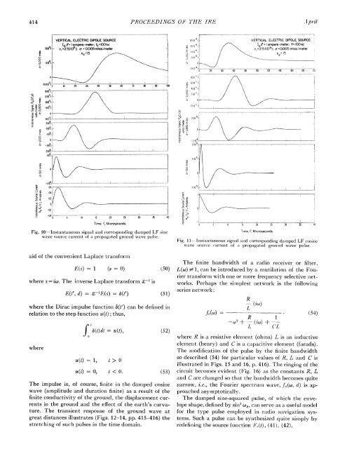
414 PROCEEDINGS OF THE IRE .1 pril Vg 1505 12001 E 8° 0'° o 4(101 2101 e 0 0e -49 -2(169) U)4) '0 10 20 30 40 50 60 70 80 90 100 |1 0. ___ _ -20A 04 z 02 - -04 .0 5 15 20 25 30 35 40 Time. t Microseconds Fig. 10-Instanltaneous signlal atod correspondliiog damped LF sinle wave soulrce currenlt of a1 propalgated groulnd ssave pullse. aid of the convenient Laplace tranisform E(s) =1 (v= 0) where s =iw. The inverse Laplace tranisform £-C is E(t', d) = £''E(s) = (t) where the Dirac impulse funlctioln 6(t') can be definied in relation to the step funictioin u(t); thus, where rt b()dt =(t), ,,j u(t)=1, I>0 (52) u(t) =O t < 0. (53) The impulse is, of course, finiite in the danmped cosine wave (amplitude and durationi finlite) as a result of the finite conductivity of the ground, the displacement currents in the ground and the effect of the earth's curvature. The transient response of the ground wave at great distances illustrates (Figs. 12-14, pp. 415-416) the stretching of such pulses in the time domain. 'E uT E V) 3C .1 -a lT -0 -3E 2 0) c el I0 400-1 2(10-I) O -2, If0 0 20 _ _ 40 VERTICAL ELECTRIC DIPOLE SOURCE 1of= ampere-meter; f=I-Okc c, =2.5(io5); o0=0.005 mhos/meter If2= 5 60 80 100 120 140 160 180 20', T IXtt ^1> 1f1^ IAX $1vX 1nt 4tir~~~~~~~~~~~~~~~~~~~~~~~~~~~~~~~ ~~~ \- \~~~~~~~~~~~~~~~~~~~~~~~~~~~~~~~~~~~~~ .S i 4 i . I~~~~~~~~~~~~~~~~~~~~~~~~~~ "I -ti - O 5 iO 15 20 25 30 35 40 Time, t Microseconds Fig. 11- Instanitanieous sigInal anid correspoindinig daniped LF cosinie xs ave souirce (current of a1 propagated gronioid wave ptulse. The finiite bandwidth of a radio receiver or filter, (50°) fr(°) #;£ 1, cani be introduced by a mutilation of the Fourier transform with onie or more frequency selective nietworks. Perhaps the simplest nietwork is the followinig f ,1\series network: (-51) fr(co) R I (ico) - R I -co2 +- (iw) + - L C'L (54) where R is a resistive elemnenit (ohms) L is an iniductive element (henry) and C is a capacitive element (farads). The n1odificationi of the pulse by the finite bandwidth so described (54) for particular values of R, L anid C is illustrated in Figs. 15 anid 16, p. 416). The ringinig of the circuit becomes evident (Fig. 16) as the constants R, L and C are changed so that the bandwidth becomes quite narrow, i.e., the Fourier spectrumii wave, fJ0(w, d) is approached asymptotically. The damped sine-squared pulse, of which the enivelope shape, defined by sinil w, can serve as a useful nmodel for the type pulse employed in radio navigation systems. Such a pulse can be syiothesized quite simiply by redefining the source funiction F,(t), (41), (42), __
Page 1 and 2: 404 PROCEEDINGS OF HIIE IRE A pril
Page 3 and 4: 406 PROCEEDINGS OF THE IRE A2 pril
Page 5 and 6: 408 PROCEEDINGS OF THE IRE .1 pril
Page 7 and 8: 410 PROCEEDINGS OF THE IRE A pril w
Page 9: 412 a,-2 .2 LL-i r 2 C: :2 Lu LL- F
Page 13 and 14: 416 l L L- O . ._ a cr, PROCEEDINGS
Page 15 and 16: 418 PROCEEDINGS OF T'HE IRE .gA pri
Page 17 and 18: 420 ELECTRON DENSITY, EL/CC Fig. 19
Page 19 and 20: 422 PROCEEDINGS OF THE IRE A pril H
Page 21 and 22: 424 a2,6 = -a i,6 exp [-i lre (2) a
Page 23 and 24: 426 The analytic expressions for th

Propagation Low-Frequency

Create successful ePaper yourself

Delete template?

Save as template?