Propagation Low-Frequency

1962
ll
((I2)I
0
Johler: Propagation of Low-Frequency Signal
14(0-13)
12 (10-13)
to 0(i0-')
1 8 (10 13)
E 6 (10 13)
0
< 4(1003)
-n iti" 12~ I]
x 2(10 13)
3(0) 0KO
20
E */\) - 0-13) II
- 10
0
4(109° } 2(10- °
tW 2(109) ~2(1°-!3 f\
-(20-9) -((010)
-E E 20Lo OO-p °
0 0n
0~~~~~~~~~~~~~~~~~~~~~~~~~~~~~~~~~~~~~~~~~~~~~~~~~~~~0
__9_
A? E
0
to
0.5
0
I
60 80 100 120 40 160 10 200
Time, t' Microseconds
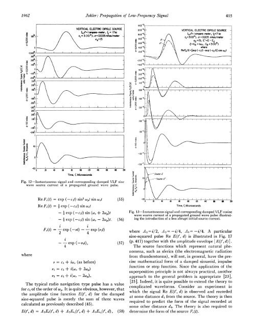
Fig. 12-IInstantaneous signal and correspondinig damped VLF sine
wave source current of a propagated ground wave pulse.
where
-nhS
0 20 40
Re F0(t) = exp (-cit) sin2 o.,t sin w,t
Re F,(t) = 1 exp (- cit) sincot
-_ exp (-c1t) sin (w, + 2cow)t
-4 exp (-cit) sin (wc - 2co)t.
Fs(t) = - exp (-Pt)- -
i i
2 4
exp (vpt)
(55)
(56)
--exp (-V2t), (57)
4
= cl + iwc (as before)
Vo = C1 + i(w, + 2wo)
P2 =
C1
.I
+ i(cw,- 2p).
VERTICAL ELECTRIC DIPOLE SOURCE
I I l-I aTr e-meter; fc - 17kc
cl - 3(104);cr- 0,005 mhos/meter -
P.215
The typical radio navigation type pulse has a value
for cl of the order of cop. It is quite obvious, however, that
the amplitude time function E(t', d) for the damped
sine-squared pulse is merely the sum of three waves
calculated as previously described (45).
E(t', d) = AI E,(t', d) + A2Ep,(t', d) + A 3E,,(t', d), (58)
c
0?
0 1._
, Lu
n; E
us -r
w ,r
a 4>
cE x
R
F-..
7.
.I
V.Vi AAI
20 0 40 60 s0 (00 120 140 0 U10 200
Time, t. Microseconds
415
VERTICAL ELECTRIC DIPOLE SOURCE -
10o = ampere-meter; fc- 17 kc
cl=3(104). a- = 0005 mhos/meter
E- /~. \ s2=15; E'=E-Ec
E-6C,
-\t=C2+iwc, C2=3(O3 -
where-
Re Fs (t) =[exp (-c1t) - exp (-c21)] cos wCt
E
----.qource E'
Fig. 13-Instantaneous signal and corresponding damped VLF cosine
wave source current of a propagated ground wave pulse illustrating
the introduction of a less abrupt initial source current.
where A i = i/2, A2 =-i/4, A3 =-i/4. A particular
sine-squared pulse Re E(t', d) is illustrated in Fig. 17
(p. 417) together with the amplitude envelope E(t', d) |.
The source functions which represent natural phenomena,
such as sferics (the electromagnetic radiation
from thunderstorms), will not, in general, have the precise
mathematical form of a damped sinusoid, impulse
function or step function. Since the application of the
superposition principle is not always practical, another
approach to the general problem is appropriate [23],
[25]. Indeed, it is quite possible to extend the theory to
complicated waveforms. Consider an experiment in
which the signal Re E(t', d) is observed and recorded
at some distance d, from the source. The theory is then
required to predict the form of the signal recorded at
some other distance d2. The theory is also required to
determine the form of the source F8(t).
II