Propagation Low-Frequency

More documents

Recommendations

Info

1962 Johler: Propagation of Low- Frequency Signal 419 has beeni treated by approximating the medium with one or more slabs of uniform compositioni as exemplified by the works of Brekhovskikh [29], Hines [30], Ferraro and Gibbon [31 J. Such methods have been exploited by Johler and Harper [27], and carried to the limit, such that the number of slabs p for each calculation depends upon the computation precision required and the particular values of the electric and geometric paranmeters. The detailed structture of such a flexible model is illustrated in Fig. 18 as a stack of plasma slabs of arbitrary thickness (but consistent with computation efficiency) zn except the topmost slab of thickness zp= co. The number of such slabs p is also quite flexible, since the notion is implied in such a model that the measured electron density-altitude, N(h) or N(z) profile, and collision frequency altitude, v(h) or v(z) profile, can be approximated to any desired accuracy by decreasing zn and increasing p simultaneously until a stable reflection process is obtained. A constant electron density and collision frequency with respect to altitude z is of course assumed for each slab. A set of four roots -=v of (71) are found to exist in each slab. Two of the roots will exhibit a negative imaginary (Im ¢ negative) corresponding to an upgoing wave (+z direction, Figs. 5 and 18) and two of these roots will correspond to a positive imaginary (Im r positive) corresponding to a downgoing wave (-z direction, Figs. 5 and 18). It is necessary to consider both upgoing and downgoing waves in the analysis of either the ~at,la,,2ai, 3a,,4al,,6al ,6 bl,lbl,2bl,,3b1,41b,5b1,6 C1,iCl,2il,3C1,4C1,5C1,6 dl,ldl,2d,,3dl,4 d,,5d,,6 a2,3(a2,4 a2,5 a2,6 a2,7a2,8 a2,9a2,l0 b2,3b2,4b2,51b2,6b2,7b2,8b2,9b2,10 C2,3C2,4C2,5C2,6C2,7C2,8 C2,9C2,10 d4,3d2,4d2,5d2,6d2,7d2,8 d2, d2,10 a3,7(a3,8(a3,9a3, 0la3,l1 a3,2 a3,13 a3,14 b3,7b3,8b3,9b3, l0b3, l1b3,12b3,13b3,14 C3,7C3,8C3,9C3,10C3,11 C3,12C3,13C3,14 d3,7d3,8d3,9d3,l0d3,11 d3,12d3,13d3,14 Cp,p+4 . reflection or transmission process at the ioniosphere, except for the topmost slab, where only the upgoing waves are considered. It is necessary to distiniguish between the ordiniary and extraordinary magneto-ionic componients of propagation for both the upgoing anid downgoing waves. This is accomplished by an examination of the form of the index of refraction function with respect to frequency and altitude (or electron density and collision frequenicy which varies with respect to altitude). Thus, the index of refractioni v [as defined by (71), (72) ] is detailed for each frequenicy and slab zn, 7 = 7n,. The upgoing ordiniary and extraordinary 77)e and the downgoinig ordinary and extraordinary 1,7),e function conitinuity is examiined in detail as a function of frequency to determine, if any, the crossover points of the functions for each slab or electron density under consideration. The absolute distinction between ordinary and extraordinary magneto-ionic wave components [19], [27] remains quite arbitrary, but the analysis must be consistent between each slab and consistent within each slab for upgoing anid downgoing waves. 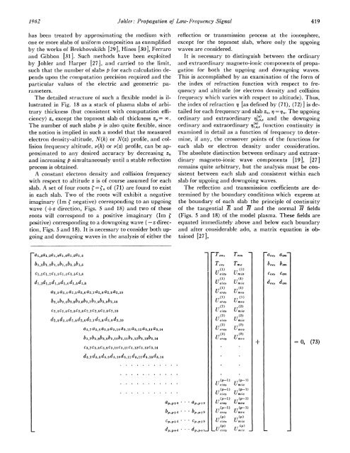The reflection and transmission coefficients are determined by the boundary conditions which express at the boundary of each slab the principle of continuity of the tangential E and H and the normal H fields (Figs. 5 and 18) of the model plasma. These fields are equated immediately above and below each boundary and after considerable ado, a matrix equation is obtained [27], . . Cp,p+9 Tein, T ee) (1) Ueioy (1) Ueio, (1) Uero) (11) Tere, (2) (2) Unie, (2) U erOy (2) Uere) u(p-i) Ueio, (p-i) Uete) (p-i) U erol (P-1) U ere (p) Ue o u(p) beic, T-M Tine (1) (1) (1) Ummo (1) Umre (2) Urnio (2) Umie (2) U mro (2) (p 1) Umio (p-I) Urnie (p-1) Umro (-) Umte- aoe) boe, Coe doe) aom born dont ± - O, (73)
420 ELECTRON DENSITY, EL/CC Fig. 19-Electron denisity-altitude [N(h) or V(z)] (quiescent and disturbed) profiles. where the elements of the matrix a1,, . . . are defined in the Appendix. The upgoing ordinary and extraordinary and the downgoing ordinary and extraordinary magneto-ionic components of propagation are coupled within the ionosphere (Fig. 18) as a result of the introduction of the boundary conditions described in concise form in the nmatrix equationi (73). Thus, at the upper and lower boundary of each slab, energy is transferred between the four magneto-ionic components of propagationi [four roots of the quartic equation (71)]. This type of coupling is distinct from the coupling of the polarization components, external to the ionosphere described previously [beginning of Sectioni V-see also Fig. 4 and (36) ]. The continuously stratified technique can be illustrated by evaluating reflections from an ionosphere inodel determined by actual measured profiles of electron density (Fig. 19) and collision frequency (Fig. 20). A typical daytime-room profile N(h) presented by Waynick [32] (Fig. 19) anid a corresponding disturbed profile of Seddoni and Jackson [33], indicative of the intensity of ioniization during a local auroral zone ioinosonde blackout, were selected for purposes of illustrating application of the described conitiniuous stratification techniques. The region of the ionosphere oni the latter curve, below 1000 electrons/cc, was represented (dashed curve, Fig. 19) with a Gaussian distribution [6], N = Nniax exp [-(z - zrnax) /k'], where the constanits N10ax, z.,I,., and k' were determined bv the measuredl profile > 1000 electronis/cc. In particular, Nmax 26,000, Zm1a, = 85,000, k' 1.92 (108). The Nicolet/3 collision frequency [34], [35] was employed in this analysis. These collision frequencies are applicable to the classical magneto-ionic theory employinlg the approximation g-v [27], [36] in the equation of motion of the electroni (70). PROCEEDINGS OF THE IRE (09 NICOLET / 3 ^-+@ \ ~~~~~~~~NN3.081' 1216 CST, 4 JULY 1957 st10 7 - \ \ \ CHURCHILL - z19551 \ CROMPTNu et cl (19531 1l06 -PWE 1\(953) 14 50 I1 60 70 g0 90 100 110 120 ALTITUDE, h, KILOMETERS Fig. 20 Collisioni frequency-altitude [v(h) or v(z)l profiles (Nicolet/3 was employed in calculations)). .11 pril The reflection coefficients T'EE, 7',0, Tlh,, aiid Twnm were evaluated (Figs. 21-28, pp. 421-422). The reflection coefficients for the quiescent profiles are illustrated in Figs. 19-25. The disturbed profiles reflection coefficienits are illustrated in Figs. 26-28. The reflection coefficients TC,1Cnj show a steadNy decrease in amplitude as the frequency is inicreased. A small perceptible rise is nioted inear the gyrofrequency, however. This was a result of the approximnationi g-v [27] and the assumed model, whereas the use of a complex collision frequency g could exhibit higher attenuation niear the gyrofrequency. Such a complex collision frequenicy can be deduced from the work of Phelps [36], Molmlud [37], Janicel anid Kahani [38], where a collisioin frequence vP=(u) proportional to the electroni energy or temperature is derived. Johler aniid Harper [27] have introduced electroni collisions proportionial to energy as a modificationi of the coefficients of the quartic equation (71). This, of course, introduces somiie changes in the detail of the reflection coefficieints, but the general formii of the reflection coefficients of the classical ihuagneto-ionic theory remains unaltered at LF/VLF. T'he miiagniitude of the abniormiial comiiponenits |en,I 6 also shows a decrement as a funictioni of frequency. These components are quite small for the assumiied imiodel ( < 0.1 at 10 kc, for examnple). The correspondintg disturbed blackout reflection coefficients imply a slight chatnge in the angle of inicideence Oi as a result of a lowerinig of the ionosphere. Ilowever, the principal cause of chanige as a result of this profile is, nievertlheless, the redistribution of the electron density-altitude profile. It is iinterestinig to niote an inlcreased aIttellUation at the higher frequencies 100 kc to 1000 kc. I-lowever, the hiigh attenuation or total ionosonde blackout which characterizes high frequencies does iiot seemli to exist at LF. Indeed, an enhancement in the field is aniticipated from this profile at VLF ( < 30 kc).
Page 1 and 2: 404 PROCEEDINGS OF HIIE IRE A pril
Page 3 and 4: 406 PROCEEDINGS OF THE IRE A2 pril
Page 5 and 6: 408 PROCEEDINGS OF THE IRE .1 pril
Page 7 and 8: 410 PROCEEDINGS OF THE IRE A pril w
Page 9 and 10: 412 a,-2 .2 LL-i r 2 C: :2 Lu LL- F
Page 11 and 12: 414 PROCEEDINGS OF THE IRE .1 pril
Page 13 and 14: 416 l L L- O . ._ a cr, PROCEEDINGS
Page 15: 418 PROCEEDINGS OF T'HE IRE .gA pri
Page 19 and 20: 422 PROCEEDINGS OF THE IRE A pril H
Page 21 and 22: 424 a2,6 = -a i,6 exp [-i lre (2) a
Page 23 and 24: 426 The analytic expressions for th

Propagation Low-Frequency

You also want an ePaper? Increase the reach of your titles

Delete template?

Save as template?