Propagation Low-Frequency

1962 Johler: Propagation of Low-Frequency Signal
417
cr
n
- l-i
a:
LD
n-
cr
t (psec)
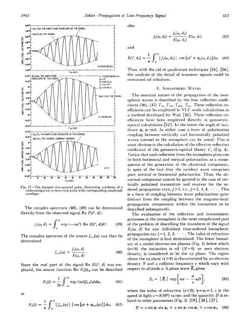
Fig. 17-The damped sine-squared pulse, illustrating synthesis of a
radio-navigationi system-type pulse with corresponding amplitude
envelope.
The complex spectrum (48), (49) can be determined
directly from the observed signal Re E(t', d):
rX
fM(w, d) = exp (-iwt') Re E(t', d)dt'. (59)
The complex spectrum of the source fx,8(wo) can then be
determined
fMw, d) (0
= E(w,d)
(60)
Since the real part of the signal Re E(t', d) was employed,
the source function Re F8(t). can be described
or
t'(fL sec)
- IFs(t)I,THE AMPLITUDE ENVELOPE OF THE SOURCE
Re Fs(t), THE SOURCE CURRENT MOMENT
ex
F,(t) = exp (x)z8Xdo
21r co
(61)
1 0x
F (t) = - f.a(W) I{cos [wt + x,a(cw)] I d@o, (62)
7ro
also
and
JxW2 ) fE(w,7
(co, di) E(w,d2)
(63)
E(t', d2) = f(, (co d2) cos [wt' + 0;(w, d.)]dcd. (64)
Thus, with the aid of quadrature techniques [24], [26],
the analysis of the detail of transient signals could be
continued ad infinitum.
V. IONOSPHERIC WAVES
The essential nature of the propagation of the ionospheric
waves is described by the four reflection coefficients
(36), (37) Tee, Tem Trrmmn Tine. These reflection coefficients
can be employed in VLF mode calculations in
a method developed by Wait [26]. T hese reflection coefficients
have been employed directly in geomnetricoptical
calculations [12 ]. In the latter the angle of incidence
Xi is real. In either case a form of polarizationi
coupling between vertically anid horizonitally polarized
waves external to the ionosphere canl be noted. This is
most obvious in the calculation of the effective reflection
coefficient of the geometric-optical theory Cj (Fig. 4).
Notice that each reflection from the ionosphere gives rise
to both horizontal and vertical polarization as a conisequence
of the generation of the abnormal componenit,
in spite of the fact that the incident wave comprises
pure vertical or horizontal polarization. Thus, the abnormal
component cannot be ignored in the case of vertically
polarized transmitter and receiver for the ordered
propagation rays, j> 1, i.e., j= 2, 3, 4, . This
is a form of coupling between wave polarizations quite
distinct from the coupling between the magneto-ionic
propagation components within the ionosphere to be
described subsequently.
The evaluation of the reflection and transmission
processes at the ionosphere is the most complicated part
of the problem of describing the transform of the signal
Ej(co, d) for any individual time-ordered ionospheric
propagation ray j= 1, 2, 3, . . The index of refraction
of the ionosphere is first determined. The lower boundary
of a model electron-ion plasma (Fig. 5) below which
(z 0) is characterized by an electron
density N and a collision frequency v which vary with
respect to altitude z. A plane wave Ei gives
Ei =
|IiI
exp [iwt D
(65)
where the index of refraction (z