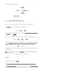
CHAPTER II DIMENSION In the present chapter we investigate ...

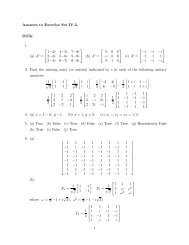
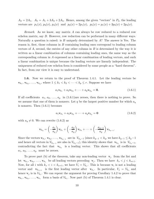
A2 = 2A1, A5 = A1 + 3A3 + 2A4. Hence, among the given “vectors” in P3, the leading
vectors are p1(x), p3(x), p4(x) and p2(x) = 2p1(x), p5(x) = p1(x) + 3p3(x) + 2p4(x).
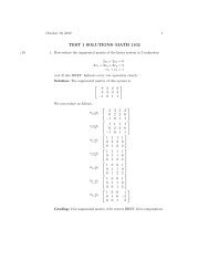
Remark. As we know, any matrix A can always be row reduced to a reduced row
echelon matrix, say B. However, row reduction can be performed in many different ways.
Naturally a question is raised: is B uniquely determined by A? The answer is Yes. The
reason is, first, those columns in B containing leading ones correspond to leading column
vectors of A, second, the entries of any other column in B is determined by the way it is
written as a linear combination of columns containing leading ones, the same way as the
corresponding column in A expressed as a linear combination of leading vectors, and such
a linear combination is unique because the leading vectors are linearly independent. The
uniqueness of reduced row echelon form is considered by some people as a “hard theorem”.
In fact, from our view it is easy to understand.
1.6. Now we return to the proof of Theorem 1.4.1. Let the leading vectors be
vk1 , vk2 , . . . , vkp , where 1 ≤ k1 < k2 < · · · < kp ≤ r. Suppose we have
a1vk1 + a2vk2 + · · · + apvkp = 0. (1.6.1)
If all coefficients a1, a2, . . . , ap in (1.6.1)are zeroes, then there is nothing to prove. So
we assume that one of them is nonzero. Let q be the largest positive number for which aq
is nonzero. Then (1.6.1) becomes
with aq = 0. We can rewrite (1.6.2) as
vkq =
a1vk1 + a2vk2 + · · · + aqvkq = 0 (1.6.2)
− a1
vk1
aq
+
− a2
vk2 + · · · + −
aq
aq−1
vkq− 1
aq
.
Since the vectors vk1 , vk2 , . . . , vkq− 1 are in Vkq−1 (since kq−1 < kq, we have kq−1 ≤ kq −1
and hence all vectors in Vkq− 1 are also in Vkq−1), this identity shows that vkq is in Vkq−1,
contradicting the fact that vkq is a leading vector. This shows that all coefficients
a1, a2, . . . , ap must be zeroes.
To prove part (b) of the theorem, take any non-leading vector vj from the list and
let vk1, vk2, . . . , vks be all leading vectors preceding vj. Then we have ks < j < ks+ 1.
Now, for all i with ks < i < ks+ 1, we have Vi = Vks . This is because vi is not a leading
vector and vks+1 is the first leading vector after vks . In particular, Vj = Vks and
hence vj is in Vks . We can repeat the argument for proving Corollary 1.4.2 to prove that
vk1 , vk2 , . . . , vks form a basis of Vks . Now part (b) of Theorem 1.4.1 is clear.
10