CHAPTER II DIMENSION In the present chapter we investigate ...

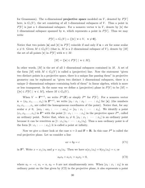
for Grassmann). The n-dimensional projective space modeled on V , denoted by P [V ]
here, is G1(V ), the set consisting of all 1-dimensional subspaces of V . Thus a point in
P [V ] is just a 1–dimensional subspace. For a nonzero vector v in V , denote by [v] the
1–dimensional subspace spanned by v, which represents a point in P [V ]. Thus we may
write
P [V ] = G1(V ) = {[v] | v ∈ V, v = 0}.
Notice that two points [u] and [v] in P [V ] coincide if and only if u = av for some scalar
a = 0. Given M ∈ G2(V ) (that is, M is a 2–dimensional subspace of V ), denote by [M]
the set of all points [v] in P [V ] with v ∈ M:
[M] = {[v] ∈ P [V ] | v ∈ M}.
In other words, [M] is the set of all 1–dimensional subspaces contained in M. A set of
the form [M] with M ∈ G2(V ) is called a (projective) line. Now the statement “given
two distinct points in a projective space, there is a unique line passing them” in projective
geometry can be rephrased as “given two distinct 1–dimensional subspaces, there is a
unique 2–dimensional subspace containing both of them” in linear algebra, which is more
or less transparent. In the same way we define a (projective) plane in P [V ] to be [M] =
{[v] ∈ P [V ] | v ∈ M}, where M ∈ G3(V ).
When V = F n+ 1 , we write P n (F) or simply P n for P [V ]. For a nonzero vector
x = (x0, x1, . . . , xn) in F n+ 1 , we write [x0 : x1 : x2 : · · · : xn] for [x]; (the numbers
x0, x1, . . . , xn are called the homogeneous coordinates of the point). Notice that, for any
scalar a = 0, [ax0 : ax1 : · · · : axn] = [x0 : x1 : · · · : xn]. We identify a point
(x1, x2, . . . , xn) in F n with the point [1 : x1 : · · · : xn] in the projective space P n , called
an ordinary point. Notice that, when x0 = 0, [x0 : x1 : · · · : xn] is an ordinary point
because it can be rewritten as [1 : x1/x0 : · · · : xn/x0]. Thus a non–ordinary point is of
the form [0 : x1 : · · · : xn]; it is called a point at infinity.
Now we give a closer look at the case n = 2 and F = R. In this case P 2 is called the
real projective plane. Let us consider a line
ax + by = c (C1)
in F 2 . Write x = x1/x0 and y = x2/x0. Then we have a(x1/x0) + b(x2/x0) = c, or
a0x0 + a1x1 + a2x2 = 0, (C2)
where a0 = −c, a1 = a, a2 = b are not simultaneously zero. When [x0 : x1 : x2] is an
ordinary point on the line given by (C2) in the projective plane, it also represents a point
30