CHAPTER II DIMENSION In the present chapter we investigate ...
CHAPTER II DIMENSION In the present chapter we investigate ...
CHAPTER II DIMENSION In the present chapter we investigate ...

Create successful ePaper yourself
Turn your PDF publications into a flip-book with our unique Google optimized e-Paper software.
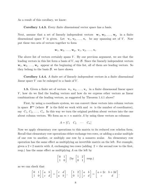
As a result of this corollary, <strong>we</strong> know:<br />
Corollary 1.4.3. Every finite dimensional vector space has a basis.<br />
Next, assume that a set of linearly independent vectors w1, w2, . . . , wp in a finite<br />
dimensional space V is given. Let v1, v2, . . . , vr be any spanning set of V . Now<br />
put <strong>the</strong>se two sets of vectors toge<strong>the</strong>r to form<br />
w1, w2, . . . , wp, v1, v2, . . . , vr<br />
The above list of vectors certainly spans V . By our previous argument, <strong>we</strong> see that <strong>the</strong><br />
leading vectors in this list form a basis of V , say B. Since <strong>the</strong> linearly independent vectors<br />
w1, w2, . . . , wp appear at <strong>the</strong> beginning of this list, all of <strong>the</strong>m are leading vectors. So<br />
<strong>the</strong>y belong to <strong>the</strong> basis B. <strong>we</strong> have shown<br />
Corollary 1.4.4. A finite set of linearly independent vectors in a finite dimensional<br />
linear space V can be enlarged to a basis of V .<br />
1.5. Given a finite set of vectors v1, v2, . . . , vn in a finite dimensonal linear space<br />
V , how do <strong>we</strong> find <strong>the</strong> leading vectors and how do <strong>we</strong> express o<strong>the</strong>r vectors as linear<br />
combinations of <strong>the</strong> leading vectors, as suggested by Theorem 1.4.1 above?<br />
First, by using a coordinate system, <strong>we</strong> can convert <strong>the</strong>se vectors into column vectors<br />
in space F m (where F is <strong>the</strong> field <strong>we</strong> work with and m is <strong>the</strong> number of coordinates),<br />
say C1, C2, . . . , Cn. <strong>In</strong> this way <strong>we</strong> turn <strong>the</strong> original problem about vectors into <strong>the</strong> one<br />
about column vectors. We form an m × n matrix A by using <strong>the</strong>se vectors as columns:<br />
A = [C1 C2 · · · Cn]<br />
Now <strong>we</strong> apply elementary row operations to this matrix to its reduced row echelon form.<br />
Recall that elementary row operations ei<strong>the</strong>r exchange two rows, or adding a scalar multiple<br />
of one row to ano<strong>the</strong>r, or multiply one row by a nonzero scalar. An elementary row<br />
operation has <strong>the</strong> same effect as multiplying an invertible matrix on <strong>the</strong> left. For example,<br />
given a 2 × 2 matrix with A, exchanging two rows (adding 2 × <strong>the</strong> second row to <strong>the</strong> first,<br />
resp.) has <strong>the</strong> same effect as multiplying A on <strong>the</strong> left by<br />
as <strong>we</strong> can check that<br />
<br />
0<br />
<br />
1 a<br />
<br />
b<br />
1 0 c d<br />
=<br />
<br />
0 1<br />
1 0<br />
<br />
c d<br />
,<br />
a b<br />
(by<br />
<br />
1 2<br />
0 1<br />
resp.)<br />
<br />
1 2 a b<br />
=<br />
0 1 c d<br />
8<br />
<br />
a + 2c b + 2d<br />
.<br />
c d