Phys. Rev. A - Victor S. L'vov Home-page - Weizmann Institute of ...

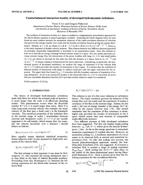
PHYSICAL REVIEW A VOLUME 46, NUMBER 8 15 OCTOBER 1992
Counterbalanced interaction locality of developed hydrodynamic turbulence
Victor L'vov and Gregory Falkovich
Department of Nuclear Physics, Weizmann Institute of Science, Rehovot 76100, Israel
and Institute of Automation, Academy of Science of Russia, Novosibirsk, Russia
(Received 18 December 199 1)
The problem of interaction locality in k space is studied in a diagrammatic perturbation approach for
the Navier-Stokes equation in quasi-Lagrangian variables. Analyzing the whole diagram series we have
found an exact relation between the asymptotic behavior of the triple-correlation function of velocities
that governs the energy transfer over scales and the double-correlation function giving the energy distri-

46 COUNTERBALANCED INTERACTION LOCALITY OF.. . 4763
Here the measure of the different scalings dp( h) is sup-
posed to be smooth. The exponent 3 - D (h ) defines the
probability of finding the scaling exponent h. The mul-
tifractality concept also gives a power behavior for all
correlation functions: since in (4) the smallest exponent
dominates in the limit of 2-0, then the correlators
behave by the power laws
though with an anomalous scaling defining by an unknown
function D (h ).
Both above pictures imply (3) and are based thus on
the locality assumption. The locality problem was studied
previously for the single-scaling Kolmogorov spectrum
only. It is done in the framework of the directinteraction
approximation [7] and in the entire perturbation
series without any cutoff [8]. Here we solve the general
locality problem without any assumptions about the
steady spectrum except (3) and scale invariance.
To analyze the mechanism of interaction balance, one
should know the triple moment for noncoinciding arguments
like
In Sec. 11, we find the asymptotic behavior of (6) for one
distance being much smaller than others. To find such
asymptotic behavior, one should use the exact formulas
for the correlation functions which are obtained by
analyzing the entire perturbation series (without any
cutoff) for the Navier-Stokes equation. Neither the di-
mensional approach nor finite closures could give the
correct answer in this case. We thus find the second [in
addition to (3)] exact relation for the asymptotic behavior
of the triple-correlation function. This relation allows us
to give in Sec. I11 the whole analysis of the interaction lo-
cality. In particular, we analyze the multifractal picture
directly in the framework of the Navier-Stokes equation.
The possible presence of different exponents gives rise to
a new question in the locality consideration. Is it possible
that locality is violated in the ultraviolet region for
sufficiently small h and in the infrared region for large h?
We show that locality analysis gives the upper restriction
for exponent h.
11. EXACT RELATION
FOR THE TRIPLE-CORRELATION FUNCTION
A natural way to analyze an interaction locality is to
consider the Navier-Stokes equation (NSE) for in-
compressible fluid flow in the k representation [2]:
where r is the Eulerian vertex and P is the transverse pro-
jector.
Equation (7) is nonlinear. Multiplying it by different
powers of velocity v (k, t ) and averaging, one could obtain
the equations for the correlation functions of the velocity
field. Time evolution of the nth correlation function is
governed by some integral with the correlation function
of order n + 1. As a first step, one could consider the
simultaneous double-correlation function
which describes the energy density over scales:
E (k, t) = k 'F( k, t ). Here angular brackets denote tur-
bulent ensemble averaging. The equation for Fa8 is as
follows:
Here F'~' is the simultaneous triple correlator:
From the physical viewpoint, the interaction locality
means that the main effect on the behavior of given k-
eddies (eddies of spatial scale 1 /k) arises because of their
interaction with eddies of the same order of size.
Mathematically, it means that the main contribution to
the integral (10) arises from the regions where q and p are
of order of k which means the convergence of the integral
(10) and nothing else. There exist different definitions of
locality separating, for instance, the case with the main
contribution from the region (k/2,2k) from the case
with that of the region (k /5,5k), etc. To our mind, such
a difference is of no principal importance for turbulence
theory, whereas the difference between the case of a convergent
integral in (10) (where one could define the energy
flux in the k space) and the case of divergency (where
energy is transferred nonlocally) is a qualitative one. Our
definition of locality is usual in the general theory of tur-
.
bulence 191.
So the main point here is the analysis of integral convergence
and, in particular, the question about the convergence
reserve that is the law of how the contribution
of a distant region in the k space turns into zero while the
distance increases. Interaction of k-eddies with q-eddies
of much larger scales is defined by the asymptotic behavior
of ~'~'(k,~,~;t) at q

4764 VICTOR L'VOV AND GREGORY FALKOVICH 46
viding convergence of the integral. It could be shown
that the locality analysis gives the same results for the exponent
interval whatever order n 12 of correlation function
is used.
Let us recall the relations between the scaling properties
of second and third correlation functions F'~' and
F'~' in the k representation and that of S, and Sj in the r
representation. Double correlators are related as follows:
For a power function F'~'( k ) a k -y with 3 < y < 5, the
main contribution to this integral is given by the region
k -- + l/l. Therefore, in the inertial interval where
S,(I)~I~~ we havey=3+f,.
Considering the similar integral for the triple correlators
S3( 1 ) and F'~'( k,q,p ) and assuming the main contributron
to be provided by the region k = q --p -- 1 / I, we
obtain the scaling behavior
F'~'( hk, hq, hp) = h-'~'~)(k,q,p) (13)
in this region. According to the scaling hypothesis for
high-order correlations, we shall assume that relation (13)
is valid for any k,p,q from the inertial interval. For the
third correlator, we thus know the total exponent only:
but not the exponents a and b separately. Therefore, one
should analyze the equation for F'~' following from (7).
It is important to emphasize that to obtain the correct expression
for F'~', one should analyze the entire series of
perturbation theory (see the Appendix for details).
The main difference between the quasi-Lagrangian and
the conventional (in terms of the Eulerian velocity)
descriptions of turbulence is that the wave vector k is no
longer preserved in the vertex V, and the functions (9)
and (1 1) become nondiagonal in k [i.e., the correlation
functions are not proportional to 6(k,-k,)]. This is the
result of the absence of spatial uniformity of the theory
due to the explicit dependence of the QL velocity (15) on
the coordinate of the marked point r,, where sweeping is
precisely eliminated.
It is convenient to develop the turbulence description
in w representation supposing statistical properties to be
invariant with respect to a time shift. We will study
double- and triple-correlation functions of velocity field.
By analogy with (9) and (1 11, let us introduce these func-
tions for the QL velocities u(r,; k, w) in the (w,kj repre-
sentation:
The main problem here is due to the fact that integrals
over k diverge in terms of Eulerian velocity v even for the
Kolmogorov spectrum. According to Kraichnan [lo],
such a divergency is caused by the strong sweeping of the
small eddies by the largest ones, so it is irrelevant to the
problem of the locality of dynamic interaction providing
energy cascade due to an energy exchange between the
eddies.
Following Ref. [8], we will use the quasi-Lagrangian
(QL) velocity u(r,,r,t) in order to eliminate the sweeping
in the vicinity of some space point r,:
If the velocities of all particles of the fluid are identical,
the above QL velocity naturally coincides with the La-
grangian velocity of fluid particle along the actual trajec-
tory. It should be noted that Eq. (15) contains no approx-
imations, since it is just the definition of the function
v( r, t 1. Formula (15) itself represents a precise relation
between the Eulerian and quasi-Lagrangian velocities. In
terms of the quasi-Lagrangian velocity, one can adequate-
ly construct a theory of turbulence [8,11], and, in particu-
lar, find the asymptotic behavior of the triple-velocity-
correlation function.
The motion equation for u(r,,;k,t ) may be derived by
substituting (15) into (7). The resulting equation has the
form of the initial Navier-Stokes equation (7) but with
another dynamic vertex V describing only the dynamic
interaction of eddies in the QL approach to the theory of
turbulence [8,11] (see also the Appendix):
It is important to emphasize that simultaneous correla-
tion functions of the order n for QL velocities F'"' coin-
cide with the same functions of Eulerian velocities F:"'
and do not depend on r, [8,11]. Therefore, we will con-
sider the problem of triad interactions in the QL ap-
proach with the sweeping being eliminated completely.
Using then the above-mentioned coincidence, we will ob-
tain a conclusion about the behavior of simultaneous

46 COUNTERBALANCED INTERACTION LOCALITY OF. . . 4765
correlation functions of Euler velocities. In particular,
we will use the following relations for the double- and
triple-velocity-correlation functions:
integrated the expressions (1 8) and (1 9) over all of wj .
In order to find an asymptotic behavior of the simul-
taneous triple-correlation function of Eulerian velocity,
we have analyzed in the Appendix the entire diagram
~~(r~;k,q,o)do/2~=~,(k,q)=~,(k)~(k-~l , (18) series for the triple moment of QL velocity. In the
asymptotic limit k

4766 VICTOR L'VOV AND GREGORY FALKOVICH - 46
+ waD /am + . . . into (20) and integrate the additional
terms arising in (21) in the same manner. Finally, we ob-
tain the following corrections to (23):
Here a, and a, are some dimensionless constants, x being
the dynamic scaling exponent (for the Kolmogorov solution,
y = y, x = f ). For multifractal subsets with an arbitrary
h, one could obtain x = 1 - h, since the typical frequency
scales with 1 as 6v(l)/l. We shall demonstrate
below that h 5 1, so x > 0. The account of the frequency
dependence gives indeed the small corrections in each order
of the expansion in k /q. Therefore, we shall use (23)
in the further calculations.
It is important to emphasize here that 6 functions of
the frequencies in (20) are the same in both terms arising
in (20) after substituting the vertex V. This leads to the
absence of a term proportional to kXF(k) in the expansion
(23). So the main term in the asymptotic expansion
of triple-correlation function (24) is a k ' -Y@l( q )/q. The
total scaling exponent of the triple-correlation function is
y, =7 according to (14). The scaling exponent of @,,,(q)
may be thus expressed in terms of the scaling exponent y
of the double correlator
Let us allow a small digression. It is interesting to
compare z, which one would obtain in the direct-
interaction approximation [7] for the triple-correlation
function, with the above correct answer. In that approxi-
mation (see the Appendix for details)
Using (201, one has in the same way the estimation for
functions @:
Due to the scaling relation 2x +y = 5 [8,11], the same result
for z, could be easily obtained in any (finite) order of
diagrammatic perturbation theory or under the assumption
that the dynamic vertex V is not renormalized. The
value oCzo coincides with the correct result z =7-y only
on the Kolmogorov solution x = f, y = y. For example,
in the multifractality approach, y > 9, which reflects the
renormalization of the vertices for a multifractal turbulence.
We do not know now how it occurs, but we
know the total exponent of the triple correlators. So, in
order to find the scaling exponent z of large wave vectors
in the triple-velocity correlator, it is necessary to take
into account the entire diagrammatic series which leads
to a renormalization of the vertices.
The difference between the initial result of Kraichnan
[7] and the present approach is due to the fact that the
direct-interaction approximation is an uncontrolled pro-
cedure. On the contrary, we shall analyze in the Appen-
dix the whole series, find the main contribution into the
triple correlator for q >>k, and prove that the neglected
terms are small by parameter (k/q)11'3. Our approach is
thus controlled with a really small parameter. We get a
result different from that of [7]: interactions with distant
scales are counterbalanced for a real spectrum with a
constant energy flux (whatever 4, it has), not only for the
Kolmogorov solution as in the direct-interaction approxi-
mation.
Now let us briefly explain the physical meaning of the
final expressions (23) and (24). The triple-correlation
function (11) with one wave number being small in com-
parison with two others corresponds to the triple-
correlation function (26) of velocity increments between
three points in r space, with one distance being smaller
than two others: r2,=r

46 COUNTERBALANCED INTERACTION LOCALITY OF . . . 4767
ergy exchange (29), and the next term becomes essential.
This term is even under k -+ - k and is proportional to
@,( k )q ,-y. Therefore, the infrared convergence is
defined by the integral
However, for the ultraviolet integral (301, the first term
in (23) gives a nonvanishing value:
The vertex I'( k,q,q a k was substituted in both (31) and
(32).
Dividing these integrals by F(k), one obtains the esti-
mate for a typical time of the nonlinear interaction of the
k-eddy with the largest eddies
which takes place for any reliable model of turbulence
(the exponents of low-order correlators are close to those
of the single-scaling Kolmogorov picture 6, =p /3).
IV. INTERACTION LOCALITY
IN THE MULTISCALING MODEL
We assumed the interaction to be local in k space for
the multifractal picture. Now it is necessary to check
that it is true for each h subset. Mathematically, the in-
tegral convergence means that one could change the or-
der of integrations over dh and dq. One may represent in
(33) the double-correlation function as an integral over
exponents h as in (4):
and a typical time of the interaction with the smallest eddies
Substituting this into (33), we find that the integral is proportional
to the negative power of L (i.e., it converges) if
h,,, < 1. It is interesting to note that the dimension
D (h) does not arise in the final expression, since qL = 1
for the lower limit of integration. The probability of
finding the largest eddy is equal to unity for all h subsets.
As one can see, the interaction with small scales produces Multifractality plays its role for small scales only.
some turbulent viscosity since r,, a k ,.
-
The
condition h < h,,, = 1 means that the maximal velocity
First, we substitute the simple single-scaling Kolmo- gradients 6u (q ) /q qh -' become singular at R co for
gorov solution into (33) and (34) to demonstrate how it
all h subsets.
converges. In this case, ~ (k)ak-"/~ and @(q)aq-10/3
For the ultraviolet integral (34), we could not represent
by virtue of (25). Calculating (33) and (341, we determine
@(q) as an integral over dh, since it is proportional to the
that the contributions of distance regions in the k space
ratio of two correlation functions F3(q)/F(q) [see (25)
into the integral (10) governing energy exchange behave
and (28)]. So the locality analysis for the interaction of
as ( k~)-~/~ and (kq)-4/3. That law was previously obk-eddies
with much smaller scales could give us only the
tained by Kraichnan, and it demonstrates the locality of
condition (35) and nothing else. It gives no restrictions
the simple Kolmogorov solution. It is worthwhile to note
for the possible values of exponent h. Indeed, it deals
that the contributions of small and large scales decrease
only with the exponent of the double-correlation funcwith
the distance by the same law. The same is true for a
tion, which is defined as min[2h - D (h) + 31 and not by
general local steady spectrum (not necessarily with the
the minimal value of h. The point is that D (h) decreases
Kolmogorov exponent), carrying constant energy flux.
while h decreases, so however slow (for small h) the drop
Indeed, in the general multifractal picture, we have
of the correlation function is in k space, the decrease in
y =c,+ 3. The exponent of @ is defined by (25) as
the probability of finding the small eddy from that h subz
=7-y =4-5, due to the flux constancy, which fixes
set provides the interaction locality.
the exponent if the triple-correlation function. There-
One could explain the physical meaning of the above
fore, F(q) = qS2+3 while @(q) = q4-C2. Substituting these locality analysii in the following way. The aforemeninto
(33) and (341, we obtain integrals that behave in the tioned locality means that a typical interaction time
same way independently of the value of 6,: (k~)"-~ and r( k, k') for the eddies of the same order of size should be
(kr1f-52. The coincidence of the laws of decreasing con- much larger than ri,( k, 1 /L ) and ruv( k , 1 /q) The first
tributions from the largest and smallest scales was first time could be estimated as a turnover time for the k-eddy
pointed out in [12] for Kolmogorov-like spectra of wave
turbulence. Such a coincidence means that in a stationary
spectrum, the contributions to interaction of all
scales, from small to large ones, are balanced [12,9]. It
from the h subset (we put k = k')
also means that for a spectrum with constant flux, the The time of an infrared interaction is estimated as being
dynamical interaction either converges at k -0 and co or necessary for the k-eddy to be distorted noticeably by the
diverges at both limits. It is worth noting that such a bal- velocity difference AuL(k) of the large-eddy flow on the
ance does not necessarily hold for any cascade steady
spectra. For example, it is not the case for a turbulence
system with two (or more) motion integrals giving
different steady spectra, as in two-dimensional turscale
of the small one. It is thus as follows:
bulence.
It is important that this time is defined by the scale of the
The locality condition is thus
k-eddy only and is independent of its velocity (that is,

4768 VICTOR L'VOV AND GREGORY FALKOVICH 46
-
which h subset the eddy belongs to). Comparing T( k) and In conclusion, we would like to say that the range of
rir, we obtain the above locality criterion h < h,,, = 1. exponents evidently should be restricted from below. We
The consideration of an ultraviolet interaction is a bit suppose that the high-order correlation functions behave
more complicated. The interaction of the given k-eddy as if they are determined by the positive exponents only
with small kl -eddies (with 7 l k >> k) should provide [3,4]. What we have shown here is that such a restriction
some turbulent viscosity v,: should be given not by locality analysis but by the other
rU,(k,kl,h )=[k2vT(kl,h )]-I .
conditions ie.g., incompressibility [13]).
The value of viscosity should depend on the turbulence APPENDIX: DIAGRAMMATIC APPROACH
level at the place and the time under consideration. This TO THE ASYMPTOTIC BEHAVIOR
means that the viscosity depends on the velocity of the OF THE HIGH-ORDER-VELOCITY-
k-eddy which generates the small eddies. The rate of en- CORRELATION FUNCTIONS
ergy dissipation
1. The quasi-Lagrangian diagram technique
be to the local
gives the viscosity
flux sik8u3(k7h). It
Following [8,11], we use the quasi-Lagrangian (QL) velocity
u(ro,r, t) (15) in order to eliminate the sweeping in
the vicinity of some space point ro. In the (t,k) representation
these equations reproduce the original Navier-
Stokes equations (7) but with another vertex V [Eq. (1611,
which was called dynamic [8].
The detailed analysis of the Wyld diagram technique
(DT) for quasi-Lagrangian velocities was given in [8,11].
Such a diagram technique was formulated [8] in terms of
the double-velocity-correlation function for the QL velocand
the following estimate for r,,:
ities u( r,; k, o) (l7j and Green's function:
Determining the ultraviolet locality, we obtain where f is an extraneous force. Let us introduce the
r/r,,= (k, /k )'-"

Here Zy6!ro; w, q, p ) and OY6( r,; w, q, p ) are mass operators
with inflowing momentum q and outflowing momentum
p. These mass operators are represented by an
infinite series of one-particle irreducible diagrams, which
have the same form as in the Wyld diagram technique for
Eulerian velocities [15,2] but the Eulerian vertices r (7)
have to be replaced by the dynamic vertices V (16):
Here Z2, is some functional of 2n vertices V, n double-
velocity-correlation functions F, and (2n - 1 ) Green's
functions G and G*; 02, is a functional of 2n vertices V,
(n + 1) functions F, and 2( n - 1) functions G and G *.
2. Diagram series for the triple-correlation function
There are many various approximate methods for cal-
culating the double-velocity-correlation function, which
F(~)
l,a& (r0;~1,~2,~3,ki,k~,k3) = x { 1 -
COUNTERBALANCED INTERACTION LOCALITY OF. . . 4769
gives a reasonable result in the inertial interval: the
Kolmogorov-Obukhov spectrum [2,16]. The triple-
velocity-correlation function is the first object that can-
not be calculated in the conventional approaches without
complete elimination of the sweeping. Therefore, it is
reasonable to use the quasi-Lagrangian approach for
analyzing triple or higher momenta of the velocity field.
In the QL diagram technique, the triple-correlation
function (17) is represented by an infinite series of dia-
grams that has the same form as in the Wyld diagram
technique for Eulerian velocities [15,2], though with the
dynamic vertices V (1 6):
Here F~~',, is some functional of (2n + 1) vertices V,
(n +2) double-velocity-correlation functions F, and
(2n + 1) Green's functions G and G*. In Kraichnan's
direct-interaction approximation F(~'=F(,~', where
0
(A6)
12,s
Here x( denotes the sum of three terms with the following replacement of the exponents: 1-2-3-1 and
lc2c3cl. The rules for reading these diagrams are as usual. They may be recollected by comparing the diagrams
for ~ 1 with ~ ' the corresponding analytical expressions:
The diagrams for Fi3' and Fi3' look like
+[term with 1+2-+3-+l , k-q-p-k]
+[term with lt2t3tl , kcqcpek]J . (A7)

4770 VICTOR L'VOV AND GREGORY FALKOVICH - 46
Note that the integral of the expression (A7) over a,,
a,, and 0 3 gives [according to (19)] the simultaneous
correlation function and it has to be proportional to
ti( k+q+p). Unfortunately, this common property is not
satisfied in (A7). The same problem arises under the cal-
culation of the simultaneous double-correlation function
for QL velocity. To solve the problem, it is necessary to
discuss some general properties of the QL technique in
more detail. We have already mentioned that all simul-
taneous correlation functions of Eulerian and quasi-
Lagrangian velocities coincide. This fact is reflected in
(1 8) and (19) for double- and triple-velocity-correlation
functions. Fulfillment of these general requirements for
In fact, fl'3' is independent of r. However, as was stated
above, this property must be fulfilled for the entire series,
but not for each of its terms. In principle, F(3) can be
calculated with any r, but in the case of a cutoff of the diagram
series, it is reasonable to do this at rrro because
this is the point where the sweeping has been eliminated
in the best way.
Now let us consider the diagram series (A61 for F'~) in
the asymptotic limit k

is some function of kj,oj (j= 1-4) expressed according
to (A10) via complete vertices A, B, and C. In an analyti-
cal form the relation (A13) is represented by the expres-
sion (20). It is very important to note that all lines F de-
pending only on k and w are presented in (A13) explicitly.
The diagrams for D do not contain such lines. Functions
F and G in these diagrams depend on k and o via sums
like k+qf--q--p and w+w,--w,. Function D thus de-
pends on k and o analytically and may be expanded at
COUNTERBALANCED INTERACTION LOCALITY OF. . .
The diagrams (A6), (A8), and (A10) for ~ (~'(k,~,~) may small k and w into series with respect to powers of k and
be represented in the following form:
w. This point allows us to obtain the asymptotical limit
of the triple correlator in the explicit form (24).
The final relations (24) or (28) are exact, since we made
no uncontrolled approximation while analyzing the
Navier-Stokes equation. Of course, using diagrammatic
series (as well as functional integral) is a poorly defined
where
procedure from the viewpoint of rigorous mathematics.
Nevertheless, in theoretical physics it could give exact results
in fluid mechanics as well as in quantum-field theory
or statistical mechanics if one analyzes series as a whole
(or, equivalently, the function integral). For example, the
Dyson equation or Ward identities are usually obtained
in that way. Note that the relation obtained is some analog
of Ward identities in the field theory.
(All)
We are grateful to V. Lebedev for reading the
manuscript and for valuable remarks. V.L. acknowledges
support from the Meyerhoff Foundation at the
Weizmann Institute.
[I] A. N. Kolrnogorov, Dokl. Akad. Nauk SSSR 32, 16 [4] A. Vincent and M. Meneguzzi, J. Fluid Mech. 225, 1
(1941). (1991).
[2] A. S. Monin and A. M. Yaglorn, Statistical Fluid Mechan- [5] G. Parisi and U. Frisch, in Turbulence and Predictability
ics (MIT, Cambridge, MA, 1971), Vols. I and 11. in Geophysical Fluid Dynamics, Proceedings of the Inter-
[3] F. Anselmet, Y. Gagne, E. Hopfinger, and R. Antonia, J. national School of Physics "Enrico Fermi," Course
Fluid Mech. 140, 63 (1984). LXXXVII, Varenna, 1984, edited by M. Ghil, R. Benzi,

4772 VICTOR L'VOV AND GREGORY FALKOVICH
and G. Parisi (North-Holland, Amsterdam, 19851, p. 84.
[6] T. Helsey, M. Jensen, L. Kadanoff, I. Procaccia, and B.
Sraiman, Phys. Rev. A 33, 1141 (1986).
[7] R. H. Kraichnan, J. Fluid Mech. 9, 1728 (1966).
[8] V. I. Belinicher and V. S. L'vov, Zh. Eksp. Teor. Fiz. 93,
533 (1987) [Sov. Phys.-JETP 66, 303 (198711.
[9] V. Zakharov, V. L'vov, and G. Falkovich, Kolmogoroc
Spectra of Turbulence (Springer-Verlag, Berlin, 199 11, Vol.
1.
[lo] R. H. Kraichnan, J. Fluid Mech. 6,497 (1959).
[I 11 V. S. L'vov, Phys. Rep. 207, 1 (1991).
[I21 G. Falkovich, Zh. Eksp. Teor. Fiz. 93, 172 (1987) [Sov.
Phys.-JETP 66,97 (198711.
[I31 U. Frisch, Proc. R. Soc. London, Ser. A 434, 31 (1991).
[I41 V. E. Zakharov and V. S. L'vov, Izv. Vyssh. Uchebn.
Zaved. 18, 1470 (1965).
[I51 H. W. Wyld, Ann. Phys. (N.Y.) 14, 143 (1961).
[16] M. Lesieur, Turbulence in Fluids (Kluwer, London, 1990).