Analytical modeling for heat transfer in sheared flows of nanofluids
Analytical modeling for heat transfer in sheared flows of nanofluids
Analytical modeling for heat transfer in sheared flows of nanofluids

You also want an ePaper? Increase the reach of your titles
YUMPU automatically turns print PDFs into web optimized ePapers that Google loves.
PHYSICAL REVIEW E 86, 016302 (2012)<br />
<strong>Analytical</strong> <strong>model<strong>in</strong>g</strong> <strong>for</strong> <strong>heat</strong> <strong>transfer</strong> <strong>in</strong> <strong>sheared</strong> <strong>flows</strong> <strong>of</strong> nan<strong>of</strong>luids<br />
Claudio Ferrari, 1 Badr Kaoui, 2 Victor S. L’vov, 3 Itamar Procaccia, 3 Oleksii Rudenko, 2,4 J. H. M. ten Thije Boonkkamp, 4 and<br />
Federico Toschi 2,4,5<br />
1 ISIS R&D Srl, Viale G. Marconi 893, Roma I-00146, Italy<br />
2 Department <strong>of</strong> Applied Physics, E<strong>in</strong>dhoven University <strong>of</strong> Technology, E<strong>in</strong>dhoven, 5600MB, The Netherlands<br />
3 Department <strong>of</strong> Chemical Physics, The Weizmann Institute <strong>of</strong> Science, Rehovot 76100, Israel<br />
4 Department <strong>of</strong> Mathematics & Computer Science, E<strong>in</strong>dhoven University <strong>of</strong> Technology, E<strong>in</strong>dhoven, 5600MB, The Netherlands<br />
5 CNR-IAC, Via dei Taur<strong>in</strong>i 19, 00185 Rome, Italy<br />
(Received 12 April 2012; published 5 July 2012)<br />
We developed a model <strong>for</strong> the enhancement <strong>of</strong> the <strong>heat</strong> flux by spherical and elongated nanoparticles <strong>in</strong><br />
<strong>sheared</strong> lam<strong>in</strong>ar <strong>flows</strong> <strong>of</strong> nan<strong>of</strong>luids. Besides the <strong>heat</strong> flux carried by the nanoparticles, the model accounts <strong>for</strong> the<br />
contribution <strong>of</strong> their rotation to the <strong>heat</strong> flux <strong>in</strong>side and outside the particles. The rotation <strong>of</strong> the nanoparticles has a<br />
tw<strong>of</strong>old effect: it <strong>in</strong>duces a fluid advection around the particle and it strongly <strong>in</strong>fluences the statistical distribution<br />
<strong>of</strong> particle orientations. These dynamical effects, which were not <strong>in</strong>cluded <strong>in</strong> exist<strong>in</strong>g thermal models, are<br />
responsible <strong>for</strong> chang<strong>in</strong>g the thermal properties <strong>of</strong> flow<strong>in</strong>g fluids as compared to quiescent fluids. The proposed<br />
model is strongly supported by extensive numerical simulations, demonstrat<strong>in</strong>g a potential <strong>in</strong>crease <strong>of</strong> the <strong>heat</strong><br />
flux far beyond the Maxwell-Garnett limit <strong>for</strong> the spherical nanoparticles. The road ahead, which should lead<br />
toward robust predictive models <strong>of</strong> <strong>heat</strong> flux enhancement, is discussed.<br />
DOI: 10.1103/PhysRevE.86.016302 PACS number(s): 47.55.pb, 47.57.E−,47.15.−x, 44.15.+a<br />
I. INTRODUCTION<br />
The enhancement <strong>of</strong> <strong>heat</strong> <strong>transfer</strong> by embedded nanoparticles<br />
<strong>in</strong> a fluid subjected to a temperature gradient is an<br />
important issue that is expected to help <strong>in</strong> technological applications<br />
such as solar <strong>heat</strong><strong>in</strong>g, and <strong>in</strong> various cool<strong>in</strong>g devices,<br />
<strong>in</strong>clud<strong>in</strong>g m<strong>in</strong>iaturized computer processors. Accord<strong>in</strong>gly,<br />
many experiments were conducted <strong>in</strong> the past few decades<br />
[1–5]. A breakthrough announcement was made from a group<br />
at Argonne National Laboratory, who studied water and oilbased<br />
nan<strong>of</strong>luids conta<strong>in</strong><strong>in</strong>g copper oxide nanoparticles. They<br />
found an amaz<strong>in</strong>g 60% enhancement <strong>in</strong> thermal conductivity<br />
<strong>for</strong> only a 5% volume fraction <strong>of</strong> nanoparticles [6]. However,<br />
subsequent research has generated what Ref. [7] referred to as<br />
“an astonish<strong>in</strong>g spectrum <strong>of</strong> results.” Results <strong>in</strong> the literature<br />
sometimes show enhancement <strong>in</strong> the thermal conductivity<br />
compared to the prediction <strong>of</strong> the Maxwell-Garnett effectivemedium<br />
theory, and sometimes they show values that are less<br />
than that same prediction [1–5]. Confus<strong>in</strong>gly enough, these<br />
discrepancies occur even <strong>for</strong> the same fluid and the same size<br />
and composition <strong>of</strong> the nanoparticles.<br />
Some <strong>of</strong> these conflict<strong>in</strong>g results were expla<strong>in</strong>ed by either<br />
the <strong>for</strong>mation <strong>of</strong> percolated clusters <strong>of</strong> particles (<strong>for</strong> the<br />
case <strong>of</strong> enhancement with respect to the Maxwell-Garnett<br />
prediction) or by surface (Kapitza) resistance (<strong>for</strong> the case <strong>of</strong><br />
reduction with respect to the same prediction) [3]. Interest<strong>in</strong>gly<br />
enough, enhancement is typically seen <strong>in</strong> quiescent fluids, and<br />
one expects that the agglomeration <strong>of</strong> clusters will become<br />
impossible <strong>in</strong> <strong>flows</strong>, be they lam<strong>in</strong>ar or turbulent. Of course <strong>in</strong><br />
technological applications, flow<strong>in</strong>g nan<strong>of</strong>luids may be the rule<br />
rather than the exception. There<strong>for</strong>e, our aim <strong>in</strong> this article is<br />
to develop models <strong>of</strong> <strong>heat</strong> flux <strong>in</strong> flow<strong>in</strong>g nan<strong>of</strong>luids where<br />
the flow can be either lam<strong>in</strong>ar or turbulent. In such systems,<br />
we cannot expect an enhancement <strong>of</strong> <strong>heat</strong> flux due to the<br />
agglomeration <strong>of</strong> particles (at least at low volume fractions),<br />
and <strong>for</strong> the sake <strong>of</strong> simplicity we will assume that there is no<br />
Kapitza resistance. S<strong>in</strong>ce it was reported <strong>in</strong> the literature that<br />
elongated nanoparticles are superior to spheres <strong>in</strong> quiescent<br />
nan<strong>of</strong>luids [8], we will study both spheres and spheroids 1 <strong>in</strong><br />
flow<strong>in</strong>g nan<strong>of</strong>luids. We will argue that generically elongation<br />
may not be advantageous at all, and we will expla<strong>in</strong> why.<br />
For completeness, we will beg<strong>in</strong> by study<strong>in</strong>g quiescent<br />
nan<strong>of</strong>luids under a temperature gradient. We will present<br />
extensive numerical simulation that will demonstrate a very<br />
good agreement with the Maxwell-Garnett theory <strong>for</strong> spherical<br />
nanoparticles and with the generalization <strong>of</strong> Nan et al. [8]<br />
<strong>for</strong> elongated particles. In the case <strong>of</strong> flow<strong>in</strong>g nan<strong>of</strong>luid, we<br />
will <strong>of</strong>fer a model that will provide expressions <strong>for</strong> the <strong>heat</strong><br />
<strong>transfer</strong> <strong>for</strong> different values <strong>of</strong> the aspect ratio <strong>of</strong> the particles,<br />
<strong>for</strong> different volume fractions, and <strong>for</strong> lam<strong>in</strong>ar and turbulent<br />
<strong>flows</strong>.<br />
The structure <strong>of</strong> the paper is as follows. In the next section,<br />
we <strong>for</strong>mulate the problem, describe the equations <strong>of</strong> motion<br />
and the numerical procedure, and discuss the dilute suspension<br />
approximation. In Sec. III, we describe the results <strong>of</strong> numerical<br />
simulations <strong>of</strong> spherical and spheroidal particles <strong>in</strong> a fluid at<br />
rest and <strong>in</strong> a shear flow. In Sec. IV, we develop an analytical<br />
model <strong>of</strong> <strong>heat</strong> <strong>transfer</strong> characteristics, i.e., the Nusselt number,<br />
and we analyze the model predictions <strong>of</strong> <strong>heat</strong> flux enhancement<br />
<strong>in</strong> two limit<strong>in</strong>g cases <strong>of</strong> very strong Brownian diffusion and<br />
weak Brownian diffusion.<br />
II. NANOFLUIDS IN THE DILUTE LIMIT<br />
In this section, we <strong>for</strong>mulate the model <strong>for</strong> dilute nan<strong>of</strong>luids<br />
laden with elongated spheroidal nanoparticles. This <strong>in</strong>cludes<br />
the basic equation <strong>of</strong> motion <strong>for</strong> the velocity and temperature<br />
fields and the boundary conditions (with constant velocity and<br />
1 A spheroid, or an ellipsoid <strong>of</strong> revolution, is a quadric surface<br />
obta<strong>in</strong>ed by rotat<strong>in</strong>g an ellipse about one <strong>of</strong> its pr<strong>in</strong>cipal axes; <strong>in</strong><br />
other words, it is an ellipsoid with two equal semidiameters.<br />
1539-3755/2012/86(1)/016302(13) 016302-1<br />
©2012 American Physical Society
CLAUDIO FERRARI et al. PHYSICAL REVIEW E 86, 016302 (2012)<br />
temperature gradients far away from particles). We also present<br />
details <strong>of</strong> the numerical simulations and their validation.<br />
A. Formulation <strong>of</strong> the problem and the flow geometry<br />
When nan<strong>of</strong>luid is very dilute, one can disregard the effect<br />
<strong>of</strong> one particle on another and consider the nan<strong>of</strong>luid as an<br />
ensemble <strong>of</strong> non<strong>in</strong>teract<strong>in</strong>g particles [9,10]. One <strong>of</strong> these is<br />
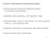
shown <strong>in</strong> Fig. 1. The center <strong>of</strong> the spheroidal particle is at<br />
the position x = y = z = 0 <strong>in</strong> the middle <strong>of</strong> a plane Couette<br />
flow between two H -separated horizontal parallel walls that<br />
move <strong>in</strong> the ˆx direction with opposite velocities V± =±V/2.<br />
Due to the symmetry, the <strong>for</strong>ces are balanced, and the particle<br />
neither migrates nor collides with the walls; the particle’s<br />
center rema<strong>in</strong>s at (0,0,0). This allows us to elim<strong>in</strong>ate <strong>in</strong> the<br />
numerics any effect <strong>of</strong> the particle sweep<strong>in</strong>g parallel to the<br />
walls. Note that this effect is absent <strong>in</strong> homogeneous cases.<br />
We employ periodic boundary conditions along the x<br />
and z direction. This results <strong>in</strong> a periodic replication <strong>of</strong> the<br />
computational box (together with the particle) <strong>in</strong> the XZ plane,<br />
lead<strong>in</strong>g to a “monolayer” <strong>of</strong> an <strong>in</strong>f<strong>in</strong>ite number <strong>of</strong> periodically<br />
distributed particles <strong>in</strong> the XZ plane. Remarkably enough (and<br />
<strong>for</strong> reasons that will be expla<strong>in</strong>ed below), this allows us to<br />
reproduce <strong>in</strong> numerics with a s<strong>in</strong>gle particle the effects <strong>of</strong> a<br />
f<strong>in</strong>ite volume fraction ϕ at least up to ϕ 20–30 %.<br />
The walls are kept at fixed temperatures T± = T ± /2.<br />
In the absence <strong>of</strong> particles, these boundary conditions give<br />
rise to a vertical temperature gradient ∇yT = /H and shear<br />
S = Sxy = V/H (see Fig. 1).<br />
The spheroidal particle’s semiaxes are a (the longest) and<br />
b (the shortest), a b (Fig. 1). The thermal diffusivity <strong>in</strong>side<br />
the particle is χp. The carrier fluid has a k<strong>in</strong>ematic viscosity<br />
ν and a thermal diffusivity χf. For simplicity, at this stage<br />
we neglect the effect <strong>of</strong> gravity and the particle mass. The<br />
H<br />
z<br />
Wall<br />
φ ~<br />
V -<br />
T+<br />
a<br />
θ<br />
y<br />
θ N<br />
T -<br />
φ<br />
V +<br />
Wall<br />
~<br />
θ<br />
b r = a/b<br />
V = S y<br />
x<br />
FIG. 1. (Color onl<strong>in</strong>e) The particle <strong>in</strong> a plane Couette flow. The<br />
largest particle axis is shown as a (red) rod. The velocity field (far from<br />
the particle) is (Sy,0,0), where the shear S = (V+ − V−)/H <strong>in</strong> the<br />
particle-free flow, with H be<strong>in</strong>g the distance between the walls. For<br />
the theoretical development, we assume the creep<strong>in</strong>g flow conditions<br />
as <strong>in</strong> [11–13].<br />
x<br />
016302-2<br />
coord<strong>in</strong>ate system and polar angles are given by<br />
nx = cos θ = s<strong>in</strong> θ s<strong>in</strong> φ, (1a)<br />
ny = s<strong>in</strong>θ s<strong>in</strong> φ = s<strong>in</strong> θ cos φ = cos θN , (1b)<br />
nz = s<strong>in</strong>θ cos φ = cos θ. (1c)<br />
We presume that n is a vector <strong>for</strong> the symmetry axis <strong>of</strong> the<br />
spheroid. Its projections onto the axis are ni, i ={x,y,z}, and<br />
θN is the angle between the particle’s largest axis and the y<br />
axis.<br />
In the absence <strong>of</strong> particles, chang<strong>in</strong>g the <strong>in</strong>tensity <strong>of</strong> the<br />
lam<strong>in</strong>ar shear flow does not change the <strong>heat</strong> flux s<strong>in</strong>ce there<br />
is no velocity orthogonal to the wall and the system is<br />
homogeneous <strong>in</strong> the direction parallel to the wall. In the<br />
presence <strong>of</strong> a particle, the shear <strong>in</strong>duces it to rotate, the<br />
simplest case be<strong>in</strong>g a spherical particle which rotates at a<br />
constant angular velocity z = S/2 (provided the particle<br />
radius is much smaller than the distance to the wall). This<br />
rotation <strong>in</strong>duces a vertical flow motion near the particle. The<br />
modification <strong>of</strong> the velocity pr<strong>of</strong>ile has three consequences.<br />
The first directly affects the <strong>heat</strong> convection <strong>in</strong> the fluid through<br />
a convective contribution vyT . The second comes from the<br />
particle rotation which br<strong>in</strong>gs up the hotter side <strong>of</strong> the particle<br />
dur<strong>in</strong>g its rotation. The third changes the <strong>heat</strong> conduction due<br />
to a modification <strong>of</strong> the temperature pr<strong>of</strong>iles at the surface <strong>of</strong><br />
the particle.<br />
In the case <strong>of</strong> nonspherical particles, the presence <strong>of</strong> a<br />
shear also has a strong <strong>in</strong>fluence on the statistical distribution<br />
<strong>of</strong> particle orientations.<br />
B. Dimensionless parameters<br />
To fix the notation, we list here the most important<br />
dimensionless parameters <strong>in</strong>volved <strong>in</strong> the problem:<br />
aspect ratio: r ≡ a/b, r 1, (2a)<br />
diffusivities ratio: k ≡ χp/χf, (2b)<br />
Prandtl number: Pr ≡ ν/χf, (2c)<br />
Reynolds number: Re ≡ (2a) 2 S/ν, (2d)<br />
Peclet number: Pe ≡ (2a) 2 S/χp. (2e)<br />
Note that the particle’s largest axis def<strong>in</strong>es our length scale.<br />
Also,<br />
Pe = Re Pr/k. (3)<br />
C. Basic equations <strong>of</strong> motion<br />
The dynamical effects previously mentioned can be studied<br />
quantitatively by solv<strong>in</strong>g the follow<strong>in</strong>g system <strong>of</strong> equations <strong>for</strong><br />
the temperature <strong>in</strong> the fluid, Tf, and <strong>in</strong> the particle, Tp:<br />
∂Tf<br />
∂t + (u · ∇)Tf = χf∇ 2 Tf,<br />
together with the boundary conditions,<br />
∂Tp<br />
∂t = χp∇ 2 Tp (4a)<br />
at the surface : Tf = Tp, χf∇Tf = χp∇Tf,<br />
on the walls: Tf(x,0,z) = T−, Tf(x,H,z) = T+.
ANALYTICAL MODELING FOR HEAT TRANSFER IN ... PHYSICAL REVIEW E 86, 016302 (2012)<br />
The fluid velocity <strong>in</strong> the whole doma<strong>in</strong> can be found by<br />
solv<strong>in</strong>g the <strong>in</strong>compressible Navier-Stokes equations:<br />
∂uf<br />
∂t + (uf · ∇)uf =− 1<br />
∇p + ν∇<br />
ρf<br />
2 uf, ∇ · uf = 0, (4b)<br />
together with nonslip boundary conditions at the surface <strong>of</strong> the<br />
particle and at the walls:<br />
uf(x,0,z) ={V−,0,0}, uf(x,H,z) ={V+,0,0},<br />
uf(x,y,z) = up(x,y,z) at the particle’s surface.<br />
Here ρf is the carrier fluid density and p is the pressure.<br />
Clearly, on nanoscales the temperature difference (across<br />
a particle) is sufficiently small to allow us to neglect the<br />
dependence <strong>of</strong> the fluid’s and particle’s material parameters<br />
on the temperature, i.e., we take ν, χf, and χp as constants.<br />
The dynamics <strong>of</strong> a neutrally buoyant particle is governed<br />
by the equations <strong>of</strong> the solid body rotation [14]:<br />
d (b)<br />
x<br />
dt<br />
d (b)<br />
y<br />
dt<br />
d (b)<br />
z<br />
dt<br />
(b) T x<br />
=<br />
Ix<br />
(b) T y<br />
=<br />
Iy<br />
(b) T z<br />
=<br />
Iz<br />
+ Iy − Iz<br />
<br />
Ix<br />
(b)<br />
y (b) z ,<br />
+ Iz − Ix<br />
<br />
Iy<br />
(b)<br />
z (b) x<br />
+ Ix − Iy<br />
<br />
Iz<br />
(b)<br />
x (b) y ,<br />
, (4c)<br />
where (b) is the angular velocity <strong>in</strong> the body-fixed frame, T (b)<br />
is the torque <strong>in</strong> the body-fixed frame, and I is the moment <strong>of</strong><br />
<strong>in</strong>ertia tensor.<br />
D. Numerical approach and its validation<br />
The numerical simulation <strong>of</strong> the conjugated <strong>heat</strong> <strong>transfer</strong><br />
problem given by Eqs. (4) is per<strong>for</strong>med by means <strong>of</strong> two<br />
coupled D3Q19 lattice Boltzmann (LB) equations under the<br />
so-called Bhatnagar-Gross-Krook (BGK) approximation [15].<br />
Details <strong>of</strong> the simulations are presented <strong>in</strong> Appendix A.<br />
Besides purely numerical means, the control <strong>of</strong> the simulations<br />
was done by its comparison with known analytical solutions.<br />
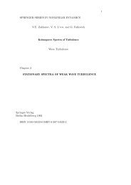
As an example, Fig. 2 shows a comparison between the<br />
analytical temperature pr<strong>of</strong>ile (A3) (solid red l<strong>in</strong>e) and the<br />
numerical pr<strong>of</strong>ile (black dots) <strong>for</strong> a moderately big spherical<br />
particle [H/(2R) = 3.2]. The second test was the comparison<br />
<strong>in</strong> Fig. 10 <strong>of</strong> the particle’s angular velocity theoretically<br />
obta<strong>in</strong>ed by Jeffery [11] and simulated by our LB realization.<br />
For more details, aga<strong>in</strong> see Appendix A.<br />
E. From s<strong>in</strong>gle-particle <strong>model<strong>in</strong>g</strong> to f<strong>in</strong>ite volume fraction<br />
Here we discuss how to relate the contribution <strong>of</strong> a s<strong>in</strong>gle<br />
particle to the <strong>heat</strong> flux with the total contribution <strong>of</strong> many<br />
weakly <strong>in</strong>teract<strong>in</strong>g particles randomly distributed <strong>in</strong> the flow<br />
occupy<strong>in</strong>g a f<strong>in</strong>ite volume fraction ϕ. The first step is to<br />
consider the fully dilute limit, ϕ → 0, <strong>in</strong> which we can<br />
exploit the fact that the particle contribution is additive and<br />
proportional to ϕ. In this way, we can <strong>in</strong>troduce the Nusselt<br />
number as the ratio between the total <strong>heat</strong> flux (<strong>in</strong>side the<br />
computational cell) and the conductive <strong>heat</strong> flux <strong>in</strong> the basic<br />
cell:<br />
Nu = 〈q〉 −χeff∇yT<br />
=<br />
〈qcond〉 −χf ∇yT<br />
χeff<br />
= , (5)<br />
χf<br />
T 0, y,0<br />
016302-3<br />
T<br />
0<br />
k Theory lbm<br />
1<br />
5<br />
100<br />
T<br />
H 2 R 0<br />
y<br />
R H 2<br />
FIG. 2. (Color onl<strong>in</strong>e) Temperature pr<strong>of</strong>ile along a l<strong>in</strong>e pass<strong>in</strong>g<br />
through the center <strong>of</strong> a spherical particle (<strong>of</strong> radius R) <strong>in</strong> a quiescent<br />
fluid. Dashed (green) l<strong>in</strong>e, conductive temperature pr<strong>of</strong>ile <strong>in</strong> the pure<br />
fluid; solid (red) curve, Eq. (A3) [16] <strong>for</strong> an <strong>in</strong>f<strong>in</strong>ite doma<strong>in</strong> with<br />
a temperature gradient; dots, numerical results (at lattice po<strong>in</strong>ts)<br />
with k = 5 (full circles) and k = 100 (squares). The present test was<br />
per<strong>for</strong>med with Pr = 1, H = 64, and R = 10 lattice units.<br />
where q is the total <strong>heat</strong> flux, qcond =−χf ∇yT is the<br />
conductive part, and χeff is the effective <strong>heat</strong> diffusivity <strong>of</strong><br />
the composite fluid. Also, ∇yT ≡ ∂T(x,y,z)/∂y. Without<br />
particles, 〈q〉 =〈qcond〉 and Nu = 1. For dilute suspensions,<br />
<strong>in</strong> which ϕ ≪ 1, Nu can be expanded <strong>in</strong> powers <strong>of</strong> ϕ [17]:<br />
Nu = 1 + ϕK(ϕ), (6a)<br />
K(ϕ) = K1 + K2 ϕ +···, (6b)<br />
where Ki are dimensionless constants dependent on the Peclet<br />
number, on the particle’s aspect ratio, r, on the relative<br />
<strong>heat</strong> diffusivity, k, and maybe other parameters such as<br />
the Reynolds or Prandtl numbers [see Eqs. (2)], i.e., Kj =<br />
Kj (Pe,r,k, . . .).<br />
As expected, <strong>in</strong> our simulations the quantity (Nu − 1) is<br />
<strong>in</strong>deed proportional to ϕ <strong>for</strong> ϕ 0.05. This allows us to f<strong>in</strong>d<br />
K1 as a function <strong>of</strong> other parameters (2) <strong>of</strong> the problem.<br />
The next-order term <strong>in</strong> the expansion (6b), i.e., K2 φ,<br />
conta<strong>in</strong>s very important <strong>in</strong><strong>for</strong>mation about how Nu depends<br />
on ϕ <strong>for</strong> small but f<strong>in</strong>ite values <strong>of</strong> ϕ. Generally speak<strong>in</strong>g,<br />
to get this <strong>in</strong><strong>for</strong>mation from numerics one needs to solve<br />
Eqs. (4) <strong>for</strong> many particles, randomly distributed <strong>in</strong> space. We<br />
demonstrate that this problem can be simplified tremendously<br />
by reduc<strong>in</strong>g it to a one-particle case, <strong>in</strong> which this particle <strong>of</strong><br />
volume V p = ϕV cell is put <strong>in</strong> the center <strong>of</strong> a computational<br />
box <strong>of</strong> volume Vcell with periodic boundary conditions <strong>in</strong> the<br />
horizontal (orthogonal to the temperature gradient) x and z<br />
directions. In this way, the total system can be considered as<br />
constructed from a periodic repetition <strong>of</strong> the basic elementary<br />
cell <strong>in</strong> the x and z directions. Compar<strong>in</strong>g <strong>in</strong> Sec. III A1<br />
our numerical results with analytical f<strong>in</strong>d<strong>in</strong>gs obta<strong>in</strong>ed under<br />
the assumption <strong>of</strong> random particle distributions, we see that<br />
<strong>for</strong> spherical particles the precise spatial distribution is not<br />
essential—what really matters is the actual volume fraction.<br />
The reason <strong>for</strong> that is quite simple: as one sees <strong>in</strong> Fig. 2,<br />
the deviation from the l<strong>in</strong>ear temperature pr<strong>of</strong>ile becomes
CLAUDIO FERRARI et al. PHYSICAL REVIEW E 86, 016302 (2012)<br />
important at distances 2 smaller than the particle diameter 2R<br />
<strong>for</strong> both k = 5 and 100. Thus any nonl<strong>in</strong>ear dependence <strong>of</strong><br />
Nu on ϕ can appear only if the particles are close enough<br />
to overlap the deviation from the l<strong>in</strong>ear temperature pr<strong>of</strong>ile.<br />
We see from our numerics that this <strong>in</strong>teraction causes a 10%<br />
deviation from the straight l<strong>in</strong>e <strong>in</strong> Nu versus the ϕ dependence<br />
<strong>for</strong> volume fractions <strong>of</strong> about 0.1 and more <strong>for</strong> k 100. For<br />
ϕ>0.1, there is some nonl<strong>in</strong>ear dependence <strong>of</strong> Nu on ϕ<br />
but it practically co<strong>in</strong>cides <strong>for</strong> the random and the periodic<br />
distributions <strong>of</strong> spherical particles. Notice that the situation<br />
is different <strong>for</strong> elongated particles: the randomness <strong>of</strong> the<br />
particle orientations is not captured by a periodic simulation.<br />
Such simulations describe only very dilute suspension, without<br />
nonl<strong>in</strong>ear effects <strong>in</strong> ϕ.<br />
III. TOWARD AN ANALYTICAL MODEL OF THE HEAT<br />
FLUX<br />
In this section, we beg<strong>in</strong> by collect<strong>in</strong>g the required <strong>in</strong><strong>for</strong>mation<br />
about the dependence <strong>of</strong> Kj on the various parameters<br />
(2). To do this we consider simple limit<strong>in</strong>g cases, <strong>for</strong> which<br />
some <strong>of</strong> these parameters are set to zero. We start with the case<br />
<strong>of</strong> spherical particles.<br />
A. Spherical nanoparticles<br />
1. Test case: spherical nanoparticles <strong>in</strong> a fluid at rest<br />
Here we consider the simplest case <strong>of</strong> a spherical particle<br />
(r = 1) <strong>in</strong> a fluid at rest (Re = Pe = 0). Chiew and Glandt [18]<br />
suggested the follow<strong>in</strong>g <strong>for</strong>mula <strong>for</strong> this case:<br />
3 K1(k)<br />
K(k,ϕ) <br />
3 − K1(k)ϕ , K1(k)<br />
k − 1<br />
= 3 , (7a)<br />
k + 2<br />
Nu = 1 + 3 K1(k) ϕ<br />
. (7b)<br />
3 − K1(k) ϕ<br />
We notice that the expression <strong>for</strong> K1(k) which controls<br />
the very dilute limit (ϕ → 0) is the same as <strong>in</strong> the Maxwell<br />
model [19]. Obviously, <strong>for</strong> k = 1 one has zero effect, i.e.,<br />
Nu = 1. For k →∞, K1 = 3 and one has maximal possible<br />
enhancement (at fixed ϕ ≪ 1). For k = 2, one has 25% <strong>of</strong> this<br />
value, k = 4 gives already 50% <strong>of</strong> the effect, k = 10 ⇒ 75%,<br />
k = 20 ⇒ 86%, and k = 100 ⇒ 97%. Clearly, the larger k the<br />
better, but <strong>in</strong>creas<strong>in</strong>g k above 100 is not effective.<br />
Actually, Eq. (7) <strong>in</strong>cludes also <strong>in</strong><strong>for</strong>mation about the<br />
nonl<strong>in</strong>ear dependence K(ϕ). However, this dependence is<br />
very weak <strong>in</strong> the relevant range <strong>of</strong> parameters: e.g., <strong>for</strong><br />
k = 10 and ϕ = 0.2 the difference between K(ϕ) and its l<strong>in</strong>ear<br />
approximation is only 15%. For smaller k, this difference is<br />
even smaller. The physical reason <strong>for</strong> that was expla<strong>in</strong>ed at the<br />
end <strong>of</strong> the preced<strong>in</strong>g section.<br />
We tested the prediction <strong>of</strong> Eq. (7) by simulat<strong>in</strong>g the <strong>heat</strong><br />
flux <strong>in</strong> a periodic box as expla<strong>in</strong>ed above <strong>in</strong> Sec. II and<br />
<strong>in</strong> Appendix A. For the fluid at rest, the (volume-averaged)<br />
Nusselt number (as a function <strong>of</strong> ϕ at different values <strong>of</strong> k)<br />
was measured and is shown <strong>in</strong> Fig. 3, where the <strong>in</strong>set shows<br />
2 It can be shown from Eq. (A3) that the distance should be smaller<br />
than R|δ −1 (k − 1)/(k + 2)| 1/3 ,whereδ is the deviation criterion, i.e.,<br />
|Tf/Tl<strong>in</strong> − 1|
ANALYTICAL MODELING FOR HEAT TRANSFER IN ... PHYSICAL REVIEW E 86, 016302 (2012)<br />
Nu Nu0 1<br />
Nu Nu0 1<br />
0.1<br />
0.01<br />
0.001<br />
10 4<br />
10 5<br />
64 3 , k 1<br />
—— Pe 2<br />
Fit II<br />
9.3<br />
14.8<br />
19.4<br />
Pe<br />
1.00<br />
10<br />
0.1 0.5 1.0 5.0 10.0 50.0 100.0<br />
0.1 0.5 1.0 5.0 10.0 50.0 100.0<br />
6<br />
0.1<br />
0.01<br />
0.001<br />
10 4<br />
10 5<br />
Data Fits<br />
k 20<br />
k 10<br />
k 5<br />
k 1<br />
LBM Runs<br />
k 20<br />
k 10<br />
k 5<br />
k 1<br />
Pe<br />
0.1<br />
10<br />
0 5 10 15 20<br />
0.1 0.2 0.5 1.0 2.0 5.0 10.0<br />
6<br />
k<br />
Pe<br />
9.3<br />
1.30<br />
1.25<br />
1.20<br />
1.15<br />
1.10<br />
1.05<br />
B 1000<br />
Nu<br />
2.0<br />
1.0<br />
0.5<br />
0.3<br />
0.2<br />
Nu Nu0 1<br />
Nu<br />
0.01<br />
0.001<br />
10 4<br />
10 5<br />
64 3 , k 5<br />
—— Pe 2<br />
1.6<br />
4.4<br />
9.3<br />
14.8<br />
19.4<br />
0.1 0.2 0.5 1.0 2.0 5.0 10.0 1.0<br />
1.1<br />
10<br />
Pe<br />
0.1 0.2 0.5 1.0 2.0 5.0 10.0<br />
6<br />
1.5<br />
1.4<br />
1.3<br />
1.2<br />
1.1<br />
Data Fits<br />
k 20<br />
k 10<br />
k 5<br />
k 1<br />
LBM Runs<br />
k 20<br />
k 10<br />
k 5<br />
k 1<br />
1.0<br />
0.1 0.2 0.5 1.0<br />
Pe<br />
2.0 5.0 10.0<br />
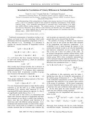
FIG. 4. (Color onl<strong>in</strong>e) . A spherical particle <strong>in</strong> a shear (Couette) flow. Upper left panel: k = 1, ϕ = 9.3%,14.8%, and 19.4%. Upper right<br />
panel: k = 5 <strong>for</strong> a wider region <strong>of</strong> ϕ, but Pe is limited by 10. Both upper panels show Nu(Pe)/Nu0 − 1 vs Pe, and both <strong>in</strong>sets show Nu(Pe) vs<br />
Pe. Here Nu0 ≡ Nu(0). Dashed (red) l<strong>in</strong>e is a fit ∝ Pe 2 , cf. Eq. (8a); (color) symbols are simulations with different volume fractions: ϕ = 1.6%,<br />
4.4%, 9.3%, 14.8%, and 19.4%. Solid (black) curve on the upper left panel represents the fit by Eq. (9). Lower panels: ϕ = 9.3% and different<br />
k (from “cold” blue, k = 1, to “hot” red, k = 20). Dashed (“temperature”-colored) l<strong>in</strong>es are fits to simulated data (symbols, same colors) by<br />
Eq. (8a), left panel, and by comb<strong>in</strong>ed Eqs. (8) and (7), right panel. Inset on lower left panel: B(k,ϕ)vsk at ϕ = 9.3%. Dot-dashed (brown) l<strong>in</strong>e<br />
is the fit to Eq. (8b). Parameters: 64 3 ,Pr= 1, thus Re = Pe k.<br />
can be fitted by<br />
B(k,ϕ) B1(ϕ) exp[B2(ϕ) k], (8b)<br />
B1 9×10 −5 ,B2 0.15. (8c)<br />
For larger Pe 10, the Nu versus Pe dependence deviates<br />
down, as expected, because at Pe →∞this dependence should<br />
saturate. Our analysis shows that this dependence can be fitted<br />
with a good accuracy by the <strong>for</strong>mula that generalizes Eq. (8a):<br />
Nu(Pe)<br />
Nu(0)<br />
− 1 <br />
B(k,ϕ) Pe 2<br />
. (9)<br />
1 + Pe/Pe1(k) + [Pe/Pe2(k)] 2<br />
The upper left panel <strong>in</strong> Fig. 4 shows by a solid (black)<br />
curve how this model works <strong>for</strong> k = 1 [with Pe1(1) ≈ 61 and<br />
Pe2(1) ≈ 63].<br />
Hav<strong>in</strong>g <strong>in</strong> m<strong>in</strong>d that <strong>in</strong> many applications related to<br />
nan<strong>of</strong>luids the value <strong>of</strong> Pe is smaller than 0.01 and <strong>in</strong> any<br />
case rarely exceeds unity, we reach the conclusion that the<br />
convective <strong>heat</strong> flux around spherical particles and variations<br />
<strong>of</strong> the <strong>heat</strong> flux <strong>in</strong>side spherical particles due to their rotation<br />
can be neglected. Equation (7) can be used to model the <strong>heat</strong><br />
flux enhanced by spherical nanoparticles with a f<strong>in</strong>ite volume<br />
016302-5<br />
fraction up to 25% and any actual value <strong>of</strong> k <strong>in</strong> fluids at rest<br />
and <strong>in</strong> shear <strong>flows</strong>.<br />
The next question to consider is the effect <strong>of</strong> the particle<br />
shape. We will beg<strong>in</strong> with the case <strong>of</strong> spheroidal particles <strong>in</strong><br />
fluids at rest.<br />
B. Spheroidal nanoparticles<br />
1. Spheroidal nanoparticles <strong>in</strong> a fluid at rest<br />
The general expectation is that spheroidal nanoparticles<br />
should be able to enhance the <strong>heat</strong> flux much more effectively<br />
than spherical particles. To achieve this, they have<br />
to be oriented <strong>in</strong> the “right” direction, i.e., along with the<br />
temperature gradient. There<strong>for</strong>e, logically, the study <strong>of</strong> the<br />
<strong>heat</strong> flux <strong>in</strong> nan<strong>of</strong>luids laden with spheroids should beg<strong>in</strong> with<br />
the clarification <strong>of</strong> the effect <strong>of</strong> the spheroid orientation on the<br />
<strong>heat</strong> flux. In this section, we consider this effect <strong>for</strong> a given<br />
and fixed orientation <strong>of</strong> the spheroids. For this purpose, we<br />
per<strong>for</strong>m numerical simulations <strong>of</strong> the <strong>heat</strong> flux with spheroidal<br />
nanoparticles <strong>in</strong> a quiescent fluid (Pe = 0) with a temperature<br />
gradient, see Fig. 1, tak<strong>in</strong>g <strong>for</strong> concreteness k = 5.<br />
For different orientations <strong>of</strong> the spheroid (i.e., different<br />
θN, the angle between the temperature gradient vector and<br />
Pe<br />
9.3<br />
1.4<br />
1.3<br />
1.2<br />
Nu
CLAUDIO FERRARI et al. PHYSICAL REVIEW E 86, 016302 (2012)<br />
Nu<br />
Nu<br />
1.30<br />
1.25<br />
1.20<br />
1.15<br />
1.10<br />
1.05<br />
1.00<br />
1.12<br />
1.11<br />
1.10<br />
1.09<br />
1.08<br />
1.07<br />
0<br />
1.06<br />
0<br />
π<br />
4<br />
π<br />
4<br />
k 5<br />
10.79 1.17 0.13 cos 2 θN<br />
4.25 1.07 0.04 cos 2 θN<br />
0.69 1.01 0.01 cos 2 θN<br />
π<br />
2<br />
k 5<br />
π<br />
2<br />
3 π<br />
4<br />
3 π<br />
4<br />
π<br />
θN<br />
4.25<br />
r 2.0<br />
π<br />
θN<br />
5 π<br />
4<br />
4.31<br />
r 2.7<br />
4.25<br />
r 2.7<br />
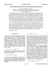
FIG. 5. (Color onl<strong>in</strong>e) Spheroid <strong>in</strong> a quiescent fluid at different<br />
angles θN. Bothpanels:k = 5, Pr = 1, 64 3 . Symbols, simulations;<br />
solid (red or blue) curves, Eq. (11) with appropriate r and ϕ; dashed<br />
(black) curves, fits by Eq. (10) to the simulations. Upper panel: r = 2.<br />
Data: ϕ 10.79% (upper), ϕ 4.25% (middle), and ϕ 0.69%<br />
(lower). The largest mismatch between the simulations and Eq. (11)<br />
is 2.8% at ϕ = 10.79%. Lower panel: lower (red) dots: ϕ = 4.25%,<br />
r = 2.0; and upper (blue) squares: ϕ = 4.31%, r = 2.7. The dotted<br />
(magenta) curve is Eq. (11) with ϕ = 4.25% and r = 2.7. The effect<br />
<strong>of</strong> chang<strong>in</strong>g r is larger than that <strong>of</strong> ϕ.<br />
the largest spheroid’s axis), we measure different Nusselt<br />
numbers: when θN = 0, spheroids with higher conductivities<br />
tend to <strong>for</strong>ms a thermal shortcut, thus Nu is larger than <strong>for</strong><br />
θN = π/2, where this shortcut effect is reduced (Fig. 5). Our<br />
numerics shows that the dependence <strong>of</strong> the Nusselt number<br />
on the spheroid orientation, i.e., Nu(θN), <strong>for</strong> small ϕ is well<br />
described by a simple <strong>for</strong>mula,<br />
5 π<br />
4<br />
3 π<br />
2<br />
3 π<br />
2<br />
7 π<br />
4<br />
7 π<br />
4<br />
2 π<br />
2 π<br />
Nu = 1 + ϕ K(k,r,ϕ,θN), (10a)<br />
K(k,r,ϕ,θN) = Km<strong>in</strong> + Kamp cos 2 (θN), (10b)<br />
and both Km<strong>in</strong> and Kamp are functions <strong>of</strong> k, r, and ϕ. This<br />
equation is a generalization <strong>of</strong> Eq. (6) <strong>for</strong> the case <strong>of</strong> spheroids,<br />
and it was suggested <strong>in</strong> [20] <strong>for</strong> the limit<strong>in</strong>g case <strong>of</strong> r →∞<br />
(nanotubes). For large ϕ>5%, deviations become visible.<br />
For f<strong>in</strong>ite ϕ, there have been attempts to study the role <strong>of</strong> the<br />
particle shape and <strong>for</strong>m factors, e.g., by Nan et al. [8]:<br />
β1 + (β2 − β1)〈cos<br />
K =<br />
2θN〉 1 − ϕ L1β1 + (L2β2 − L1β1)〈cos2 , (11)<br />
θN〉<br />
where βj = [Lj + 1/(k − 1)] −1 , j = 1,2,<br />
r>1:L1 =<br />
L2 = 1 − 2L1,<br />
r<br />
2(r 2 − 1)<br />
<br />
r − arccosh(r)<br />
<br />
√ .<br />
r2 − 1<br />
Here 〈···〉stands <strong>for</strong> an ensemble average. Clearly, <strong>in</strong> the case<br />
<strong>of</strong> a s<strong>in</strong>gle particle as <strong>in</strong> our simulations, or <strong>for</strong> a periodic array<br />
<strong>of</strong> particles, the average co<strong>in</strong>cides with the s<strong>in</strong>gle value. Notice<br />
also that <strong>for</strong> spheres, i.e., when r → 1, L1 = L2 = 1/3 and<br />
β1 = β2 = K1 from Eq. (7), and Eq. (11) simplifies to Eq. (7).<br />
For small ϕ, Eq.(11) co<strong>in</strong>cides with Eq. (10b), giv<strong>in</strong>gan<br />
analytical expression <strong>for</strong> Km<strong>in</strong> and Kamp.<br />
The range <strong>of</strong> validity <strong>of</strong> Eq. (11) was tested by means <strong>of</strong> a<br />
series <strong>of</strong> simulations at vary<strong>in</strong>g angles and volume fractions.<br />
The results are reported <strong>in</strong> Fig. 5. We can conclude that the<br />
model <strong>in</strong> Eqs. (11) well represents the <strong>heat</strong> flux <strong>in</strong> the presence<br />
<strong>of</strong> rest<strong>in</strong>g spheroidal particles <strong>in</strong> the relevant range <strong>of</strong> the<br />
parameters k, r, and ϕ. To apply Eqs. (11) <strong>for</strong> spheroids <strong>in</strong> a<br />
simple shear flow, we have to f<strong>in</strong>d how the ensemble average<br />
〈cos 2 θN〉 depends on r. For this purpose, we first need to know<br />
the orientational distribution function <strong>of</strong> spheroids <strong>in</strong> the shear<br />
flow. This is the subject <strong>of</strong> the follow<strong>in</strong>g subsection.<br />
2. Spheroidal nanoparticles <strong>in</strong> a shear flow<br />
The effect <strong>of</strong> rotation <strong>of</strong> elongated spheroidal particles<br />
(r >5) is very similar to that <strong>of</strong> spherical ones (r = 1):<br />
only the parameters B, Pe1, and Pe2 <strong>of</strong> the advanced fit (9)<br />
depend on the aspect ratio r. As an example, we presented<br />
<strong>in</strong> Fig. 6 a prelim<strong>in</strong>ary result <strong>of</strong> the computed and fitted<br />
Nu(Pe) dependence <strong>for</strong> r = 5 and k = 5. In this case, B ≈<br />
5.3 × 10⁻⁵ ,Pe1≈ 5.2, and Pe2 ≈ 30.3. This is <strong>in</strong>terest<strong>in</strong>g to<br />
compare with the respective parameters <strong>for</strong> r = 1 and k = 5:<br />
B ≈ 2.5 × 10⁻⁴ ,Pe1≈61, and Pe1 ≈ 63. One sees that the<br />
Pe enhancement <strong>of</strong> the <strong>heat</strong> flux with elongated particles<br />
is smaller than <strong>for</strong> spherical ones [B(r >1) 1) < Pe1(r = 1) and<br />
Pe2(r >1) < Pe2(r = 1). Moreover, the overall conclusion<br />
that Nu(Pe) is almost Pe-<strong>in</strong>dependent <strong>for</strong> Pe 1 rema<strong>in</strong>s valid,<br />
Nu Nu 0 1<br />
016302-6<br />
0.001<br />
5 10 4<br />
2 10 4<br />
1 10 4<br />
5 10 5<br />
2 10 5<br />
r 5<br />
k 5<br />
1<br />
0.5 1 2 3 5 10 20 30<br />
Peclet number, Pe<br />
FIG. 6. (Color onl<strong>in</strong>e) Example <strong>of</strong> advanced fit (9) <strong>for</strong> a spheroid<br />
r = 5, k = 5. (Blue) dots, numerical data; solid (red) curve, fit by<br />
Eq. (9) with B ≈ 5.3 × 10 −5 ,Pe1 ≈ 5.2, and Pe2 ≈ 30.3. Dashed<br />
(red) l<strong>in</strong>e is B Pe 2 . Here Nu is the time-averaged Nu(t) over the<br />
period <strong>of</strong> rotation (determ<strong>in</strong>ed <strong>in</strong> the simulations), and Nu0 is the<br />
time-averaged Nu(t) <strong>for</strong> the smallest available Pe, e.g., Pe = 0.01.
ANALYTICAL MODELING FOR HEAT TRANSFER IN ... PHYSICAL REVIEW E 86, 016302 (2012)<br />
thus the model developed above <strong>in</strong> Eq. (11) with Eq. (24) may<br />
be safely used <strong>for</strong> nanoparticle-laden <strong>flows</strong> at Pe 1.<br />
IV. ANALYTICAL MODEL OF HEAT TRANSFER IN<br />
A LAMINAR SHEAR FLOW<br />
In this section, we develop an analytical model <strong>for</strong><br />
Nu(k,r,ϕ).<br />
A. Orientational statistics <strong>of</strong> elongated nanoparticles<br />
1. Fokker-Planck equations <strong>for</strong> the orientational PDF<br />
In order to study the orientational statistics <strong>of</strong> elongated<br />
nanoparticles, we consider the probability distribution function<br />
(PDF), P(θ,φ,t), which is the probability P (θ,φ,t) <strong>of</strong> f<strong>in</strong>d<strong>in</strong>g<br />
any particular spheroid with its axis <strong>of</strong> revolution <strong>in</strong> the <strong>in</strong>terval<br />
[θ,θ + dθ] × [φ,φ + dφ] on the unit sphere. The PDF is then<br />
def<strong>in</strong>ed by<br />
P (θ,φ,t) = P(θ,φ,t)s<strong>in</strong>θdφdθ. (12)<br />
It was shown by Burgers [21] that P(θ,φ,t) satisfies a<br />
generalized Fokker-Planck equation <strong>in</strong> the presence <strong>of</strong> a shear:<br />
∂P<br />
∂t =−∇ · (wP) + Dr∇ 2 P, (13)<br />
where w ≡ (0, ˙θ,˙φ s<strong>in</strong> θ) is the relative velocity on the unit<br />
sphere <strong>of</strong> the axis <strong>of</strong> revolution <strong>for</strong> a particle with <strong>in</strong>stantaneous<br />
orientation (θ,φ) ignor<strong>in</strong>g all Brownian effects. The explicit<br />
<strong>for</strong>m <strong>of</strong> this equation <strong>in</strong> spherical coord<strong>in</strong>ates is<br />
∂P(θ,φ)<br />
∂t<br />
+ 1<br />
<br />
∂<br />
s<strong>in</strong> θ ∂θ Fθ s<strong>in</strong> θ + ∂<br />
∂φ Fφ<br />
<br />
= 0. (14a)<br />
Here Fθ and Fφ are the θ and φ projections <strong>of</strong> the probability<br />
density fluxes that have two shear-<strong>in</strong>duced contributions, one<br />
proportional to w and the other to the rotational diffusion<br />
coefficient, Dr:<br />
Fθ =<br />
Fφ =<br />
<br />
∂θ ∂<br />
− Dr P(θ,φ), (14b)<br />
∂t ∂θ<br />
<br />
s<strong>in</strong> θ ∂φ<br />
<br />
Dr ∂<br />
− P(θ,φ). (14c)<br />
∂t s<strong>in</strong> θ ∂φ<br />
Burgers <strong>in</strong> Ref. [21] derived the rotational diffusion<br />
coefficient, Dr, <strong>of</strong> elongated rigid spheroids <strong>of</strong> revolution:<br />
Dr = kBT 2 r + 1<br />
4μV r2 −1 . (15a)<br />
K3 + K1<br />
Here μ is the dynamical fluid viscosity, k B = 1.374 ×<br />
10 −16 erg/deg K is the Boltzmann constant, particle volume<br />
016302-7<br />
V = 4<br />
3πa2b,2a = d, b = ra, r 1, and<br />
∞ rdx<br />
K3 =<br />
0 (r2 + x) 3/2 (15b)<br />
(1 + x)<br />
= 2<br />
r2 <br />
<br />
r arccosh(r) ln(2 r/e)<br />
1 − √ → 2<br />
− 1 r2 − 1 r2 ,<br />
∞ rdx<br />
K1 =<br />
0 (r2 + x) 1/2 (1 + x) 2<br />
= r<br />
r2 <br />
r −<br />
− 1<br />
arccosh(r)<br />
<br />
√ → 1. (15c)<br />
r2 − 1<br />
This asymptotics is <strong>for</strong>mally valid <strong>for</strong> r ≫ 1, but gives<br />
better than 10% accuracy already <strong>for</strong> r>4, allow<strong>in</strong>g us to<br />
suggest the approximate “practical” <strong>for</strong>mula<br />
Dr Dr = k B T<br />
4μV<br />
ln(4r2 /e)<br />
(r2 , (16)<br />
+ 2 r/3 − 1)<br />
which works with an accuracy <strong>of</strong> about 10% <strong>for</strong> any r 1 and<br />
with better than 5% accuracy <strong>for</strong> r>10.<br />
The complete analysis <strong>of</strong> Eqs. (14) is very <strong>in</strong>volved; see,<br />
e.g., Refs. [12] and [13]. We consider only the small-diffusion<br />
limit; see the next subsection.<br />
2. Statistics <strong>of</strong> elongated nanoparticles <strong>in</strong> the small-diffusion limit<br />
Jeffery [11] has shown that if <strong>in</strong>ertial and Brownian motion<br />
affects are completely neglected, then the motion <strong>of</strong> the axis<br />
<strong>of</strong> revolution <strong>of</strong> a spheroidal particle is described by<br />
tan φ = r tan τ, (17a)<br />
tan θ = C cos2 τ + r2 s<strong>in</strong>2 τ<br />
= Cr(r 2 cos 2 φ + s<strong>in</strong> 2 φ) −1/2 , (17b)<br />
where τ = t/Tr with Tr = (r + 1/r)/S, and the constant <strong>of</strong><br />
<strong>in</strong>tegration C is called the (Jeffery) orbit constant.<br />
To analyze the small-diffusion limit, we <strong>in</strong>troduce two<br />
time scales. The first one def<strong>in</strong>es the periodic motion that<br />
a nanoparticle with a f<strong>in</strong>ite r exhibits: Tr = TJ/2π, where<br />
TJ = 2π(r + 1/r)/S is the Jeffery’s period. The second time<br />
scale is determ<strong>in</strong>ed by the <strong>in</strong>verse shear, TS = S−1 . Clearly,<br />
<strong>for</strong> large r this is a much shorter time scale, so <strong>for</strong> r ≫ 1,<br />
Tr ≈ r/S = rTS. (18)<br />
It means that the particles spend most <strong>of</strong> their time near pre- and<br />
postaligned states. If the Brownian diffusion is small enough<br />
such that Tdif = D−1 r ≫ Tr, one can neglect the effect <strong>of</strong> the<br />
Brownian motion on the dynamic motions <strong>of</strong> particles along<br />
Jeffery orbits [11] even dur<strong>in</strong>g their slow time evolution. In<br />
this case, the stationary Fokker-Planck equation (13) takes the<br />
simple <strong>for</strong>m<br />
∇ · (wP) = 0. (19)<br />
This equation can be solved [12,13] giv<strong>in</strong>g<br />
P(θ,φ) = f (C,r) PC(θ,φ), (20a)<br />
PC(θ,φ) = (r s<strong>in</strong> θ cos 2 θ cos2φ + s<strong>in</strong>2φ/r2 ) −1 , (20b)<br />
where PC(θ,φ) is the PDF along a particular Jeffery orbit with<br />
a given <strong>in</strong>tegration constant C, and f (C,r) is the probability
CLAUDIO FERRARI et al. PHYSICAL REVIEW E 86, 016302 (2012)<br />
to occupy this orbit. This function is normalized as follows:<br />
∞<br />
f (C)dC =<br />
0<br />
1<br />
4π .<br />
f (C,r) was found <strong>in</strong> [12] <strong>for</strong> the follow<strong>in</strong>g limit<strong>in</strong>g cases:<br />
f (C,r = 1) = 1 C<br />
4π (C2 , (21a)<br />
+ 1) 3/2<br />
f (C,r ≫ 1) 1 C<br />
π (4C2 , (21b)<br />
+ 1) 3/2<br />
f (C,r ≪ 1) 1 Cr<br />
π<br />
2<br />
(4r2C 2 . (21c)<br />
+ 1) 3/2<br />
Note that Eq. (21a) is exact, provid<strong>in</strong>g a consistency check<br />
<strong>of</strong> the present approach by comparison with spherical particles.<br />
The asymptotic, Eq. (21b), is very accurate <strong>for</strong> r>20, but<br />
already <strong>for</strong> r 4 it provides reasonable accuracy (better than<br />
∼ 10%).<br />
The analysis <strong>of</strong> Eqs. (21) together with the available<br />
numerical solutions <strong>for</strong> r = 0.26 and 3.86 [12] allowed us<br />
to suggest the follow<strong>in</strong>g approximation:<br />
C/(r + 1/r)<br />
f (C,r) <br />
2<br />
π 1 + 4 C2 /(r + 1/r) 2 . (22)<br />
3/2<br />
A comparison <strong>of</strong> this approximation with the exact numerical<br />
solution provided <strong>in</strong> Ref. [12] is presented <strong>in</strong> Fig. 7, upper<br />
panel. One sees that Eq. (22) fits the numerical data with an<br />
accuracy better than 5%. This is more than enough <strong>for</strong> our<br />
purpose to <strong>of</strong>fer an approximate <strong>for</strong>mula <strong>for</strong> 〈cos2 θN〉 as a<br />
function <strong>of</strong> r; see below.<br />
Next we use the fact that Jeffery orbits do not <strong>in</strong>tersect on<br />
the unit sphere. In other words, fix<strong>in</strong>g C results <strong>in</strong> a relation<br />
between θ and φ along an orbit. This relationship is obta<strong>in</strong>ed<br />
by <strong>in</strong>vert<strong>in</strong>g Eq. (17b):<br />
C = C(θ,φ) = tan θ r −2 s<strong>in</strong> 2 φ + cos 2 φ. (23)<br />
Substitut<strong>in</strong>g this function <strong>in</strong>to any one <strong>of</strong> Eqs. (21), we<br />
get f (C,r) <strong>for</strong> a given regime <strong>of</strong> r. This is then substituted<br />
<strong>in</strong> Eqs. (20), lead<strong>in</strong>g f<strong>in</strong>ally to a solution <strong>of</strong> the<br />
orientational PDF P(θ,φ), which can be used <strong>for</strong> averag<strong>in</strong>g<br />
Eqs. (11) <strong>in</strong> the case <strong>of</strong> weak Brownian motion. As a<br />
consistency check <strong>of</strong> the approach, one can consider the trivial<br />
case r = 1. From Eq. (23) one f<strong>in</strong>ds C = tan θ, then from<br />
Eq. (21a) f (C) = s<strong>in</strong> θ cos 2 θ/4π, and f<strong>in</strong>ally from Eq. (20b)<br />
PC = 1/ s<strong>in</strong> θ cos 2 θ. As a result, one has <strong>for</strong> the sphere<br />
P = 1/4π, as expected.<br />
For moderate and strong Brownian rotational motion, the<br />
notion <strong>of</strong> separate Jeffery orbits becomes irrelevant. In this<br />
case, we need to solve Eq. (13) without approximations. Once<br />
this equation is solved, we can compute 〈cos 2 θ〉 and substitute<br />
the answer <strong>in</strong> Eqs. (11). To achieve this <strong>in</strong> the most general case<br />
is not a simple task, and here we satisfy ourselves with the two<br />
limit<strong>in</strong>g cases <strong>of</strong> very large and very small rotational diffusion.<br />
The second case was discussed above. For the case <strong>of</strong> very<br />
strong rotational diffusion, we can use the same Eqs. (11),but<br />
averaged with a uni<strong>for</strong>m PDF P(θ,φ) = 1/4π. This is because<br />
the very strong rotational diffusion tends to distribute particle<br />
motions around the Jeffery orbits uni<strong>for</strong>mly. The corrections<br />
f C,r<br />
cos 2 θ N<br />
016302-8<br />
0.06<br />
0.05<br />
0.04<br />
0.03<br />
0.02<br />
0.01<br />
r<br />
r 100<br />
r 5<br />
r 2<br />
r 1<br />
0.00<br />
0.01 0.05 0.10 0.50 1.00 5.00 10.00<br />
C<br />
0.35<br />
1 3<br />
0.30<br />
0.25<br />
0.20<br />
0.15<br />
0.10<br />
0.05<br />
0.00<br />
cos 2 θN approximation<br />
—– via f C,r approximation<br />
—— pure numerical solution<br />
5 mismatch<br />
5 10 15 20<br />
r<br />
FIG. 7. (Color onl<strong>in</strong>e) . Upper panel: Comparison <strong>of</strong> “exact<br />
numerical” solutions obta<strong>in</strong>ed from Eq. (19) (solid l<strong>in</strong>es) and approximate<br />
solutions obta<strong>in</strong>ed from Eq. (22) <strong>for</strong> different r (dashed l<strong>in</strong>es).<br />
There is a visible difference (about 5% <strong>in</strong> the value <strong>of</strong> maximum) only<br />
<strong>for</strong> r = 5. Lower panel: Comparison <strong>of</strong> the dependence <strong>of</strong> 〈cos 2 θ〉<br />
vs r obta<strong>in</strong>ed by (a) apply<strong>in</strong>g “exact numerical” PDF (black solid<br />
l<strong>in</strong>e), (b) approximate analytical PDF, Eq. (22) (red dashed l<strong>in</strong>e),<br />
and (c) analytical approximation <strong>for</strong> this dependence, Eq. (24) (blue<br />
dot-dashed l<strong>in</strong>e).<br />
up to O(S/Dr) 2 to such a uni<strong>for</strong>m distribution may be found<br />
<strong>in</strong> Refs. [22,23].<br />
B. Predictions <strong>of</strong> the model<br />
1. Spheroidal nanoparticles <strong>in</strong> a strong Brownian diffusion limit<br />
With very strong Brownian diffusion, the particles are<br />
oriented completely randomly, and 〈cos2 θN〉 =1/3. In this<br />
case, Eqs. (10) and (11) give the results reported <strong>in</strong> Fig. 8, upper<br />
panels. The upper left panel shows Nu versus r dependence<br />
<strong>for</strong> various k from 1 to 8600 and ∞ with volume fraction<br />
ϕ = 1%. These results are rather obvious: <strong>for</strong> k = 1, one<br />
obta<strong>in</strong>s Nu = 1, i.e., no enhancement; the larger the k, the<br />
larger the <strong>heat</strong> flux enhancement; <strong>for</strong> any f<strong>in</strong>ite k, there is a<br />
saturation <strong>of</strong> Nu(r) <strong>for</strong>r→∞.Thevalue<strong>of</strong>(Nu−1) may<br />
be huge <strong>for</strong> spheroids (essentially, rodlike particles at r ≫ 1),<br />
e.g., <strong>for</strong> k = 8600 (diamond <strong>in</strong> water), Nu − 1 30, while <strong>for</strong><br />
spherical particles (r = 1), Nu − 1 = 0.03 at the same volume<br />
fraction ϕ = 0.01. The values <strong>of</strong> Nu(k,r) are bounded, i.e.,<br />
Nu(1,r) Nu(k,r) Nu(∞,r).<br />
The upper right panel shows Nu versus k dependence at ϕ =<br />
1% <strong>for</strong> three values <strong>of</strong> r: 1, 5, and 10. The values <strong>of</strong> Nu(k,r)are
ANALYTICAL MODELING FOR HEAT TRANSFER IN ... PHYSICAL REVIEW E 86, 016302 (2012)<br />
Nu<br />
Nu<br />
30.0<br />
20.0<br />
10.0<br />
1<br />
k 8600<br />
k 2000<br />
k 1500<br />
k 100<br />
Nu<br />
k 10<br />
1.15<br />
1.10<br />
1.05<br />
1 3 5 7.5 10 1.00<br />
5.0<br />
r<br />
k 1<br />
3.0<br />
k<br />
k<br />
1000<br />
500<br />
2.0<br />
k<br />
k<br />
100<br />
10<br />
k 5<br />
k 1<br />
1.0<br />
1 5 10 50 100 500 1000<br />
r<br />
1.08<br />
1.06<br />
1.04<br />
1.02<br />
1.00<br />
k 5<br />
k 2<br />
k 1<br />
k 1500<br />
k 1000<br />
k 500<br />
k 100<br />
k 50<br />
k 20<br />
k 5<br />
k 2<br />
k 1<br />
1<br />
k 20<br />
k<br />
k 50<br />
k 500<br />
k<br />
k 1000<br />
k 100<br />
k 1500<br />
k 8600<br />
k 2000<br />
k 1500<br />
k 1000<br />
k 500<br />
k 100<br />
1 5 10 50 100 500<br />
r<br />
Nu<br />
Nu<br />
1.15<br />
1.10<br />
1<br />
upper bound<br />
r<br />
r 10<br />
r 5<br />
1.05<br />
r<br />
lower bound<br />
spheres<br />
1<br />
1.00<br />
1 5 10 50 100 500 1000<br />
k<br />
1.05<br />
1.04<br />
1.03<br />
1.02<br />
1.01<br />
1<br />
r 1000<br />
upper bound<br />
r ropt k<br />
lower bound<br />
r<br />
r 10<br />
r 5<br />
r 1<br />
1.00<br />
1 5 10 50 100 500 1000<br />
k<br />
FIG. 8. (Color onl<strong>in</strong>e) ϕ = 1%, r0 = 10. Upper panels: strong Brownian diffusion limit: cos2 <br />
θN → 1/3; lower panels: weak Brownian<br />
diffusion limit. Left panels: Nusselt number Nu vs particle aspect ratio r <strong>for</strong> various <strong>heat</strong> diffusivity ratios, k: solid curves <strong>for</strong> rr0 (the region where the particles may, <strong>in</strong> pr<strong>in</strong>ciple, start touch<strong>in</strong>g each other). The shaded (green) area is the region <strong>of</strong> all<br />
possible Nu(k,r) atϕ = 0.01: the lower bound is given by Nu(1,r), the upper one is Nu(∞,r). Right panels: Nu vs k <strong>for</strong> various, r. Dotted<br />
(black) curve is <strong>for</strong> r = 1, spherical particles; solid (blue) curve is <strong>for</strong> r = 5; dashed (red) curve is <strong>for</strong> r = 10; and dot-dashed (brown) curve is<br />
<strong>for</strong> r = 1000, lower panel, or r →∞, upper panel. The shaded (green) area is the region <strong>of</strong> all possible Nu(k,r)atϕ = 0.01: the lower bound<br />
is Nu[k,1] <strong>in</strong> the upper panel and Nu(k,∞) <strong>in</strong> the lower panel, while the upper bound is Nu(k,∞) <strong>in</strong> the upper panel and Nu[k,ropt(k)] <strong>in</strong> the<br />
lower panel, where ropt(k) maximizes Nu at every k; see the text <strong>for</strong> additional details. The geometrical constra<strong>in</strong> imposes 1 r max(ropt,10)<br />
<strong>for</strong> ϕ = 1%.<br />
bounded, too: Nu(k,1) Nu(k,r) Nu(r,∞). Here, the more<br />
elongated the particle is (larger r), the better the enhancement.<br />
And last but not least, elongated particles may touch each<br />
other much more easily. As we show <strong>in</strong> Appendix B, the basic<br />
geometrical requirement that the mean <strong>in</strong>terparticle distance is<br />
less than the largest particle size means that r
CLAUDIO FERRARI et al. PHYSICAL REVIEW E 86, 016302 (2012)<br />
Maximal Nu<br />
1.035<br />
1.030<br />
1.025<br />
1.020<br />
1 1.11 1.97<br />
ropt<br />
4.02 5.57 6.9 8. 9.1 10.1<br />
1<br />
theory<br />
fit<br />
10 15 20 30 50 70<br />
5 7 10 20<br />
k<br />
30 40 50 60 70<br />
k<br />
ropt<br />
10.0<br />
7.0<br />
5.0<br />
3.0<br />
2.0<br />
1.5<br />
1.0<br />
Nu, color "temperature" map<br />
0 50 100 150 200 0<br />
FIG. 9. (Color onl<strong>in</strong>e) . Weak Brownian diffusion limit, ϕ = 1%, r0 = 10. Left: The largest reachable Nusselt number, Nu(k,ropt), solid<br />
(black) curve (ropt maximizes Nu <strong>for</strong> a given k). Dashed (red) l<strong>in</strong>e is the fit by Nu fit<br />
max ≈ 1 + ϕ[0.75 + 0.66 ln(k)]. Inset: ropt vs k, solid (blue)<br />
curve, and the fit rfit opt ≈−3.03 + 1.57√k <strong>for</strong> 1 ropt 10, dashed (red) l<strong>in</strong>e. S<strong>in</strong>ce ϕ = 0.01 ≪ 1, this fit may be considered as ϕ-<strong>in</strong>dependent<br />
<strong>for</strong> ϕ 1%. Right: Contour-density plot <strong>of</strong> Nu(k,r) color-coded with the “temperature” map: the larger the value <strong>of</strong> Nu, the warmer the color;<br />
contours show isovalues <strong>of</strong> Nu. Thick (black) solid and dashed curves represent those pairs <strong>of</strong> (k,r) <strong>for</strong> which Nu is maximal [i.e., solid (blue)<br />
curve <strong>in</strong> the <strong>in</strong>set]; the solid curve is <strong>for</strong> rr0. Wide-dashed (white) curve is the rfit opt (k) fit.<br />
The lower left panel <strong>in</strong> Fig. 8 shows Nu(r) <strong>for</strong> different k<br />
and ϕ = 0.01, at which the Maxwell-Garnett limit <strong>of</strong> Nu − 1<br />
<strong>for</strong> spherical particles (r = 1) is 3ϕ = 0.03. Notice that the<br />
Nu(r) dependence is not monotonic and has a maximum at<br />
some r = ropt, which depends on k. The reason <strong>for</strong> this is the<br />
competition <strong>of</strong> two effects: more elongated nanoparticles make<br />
a larger contribution to the <strong>heat</strong> flux when their longer axis is<br />
aligned with the temperature gradient, which is orthogonal<br />
to the velocity gradient (shear) <strong>in</strong> our case. However, longer<br />
nanoparticles are affected more readily by the shear, which<br />
tends to orient them <strong>in</strong> the unfavorable direction orthogonal<br />
to the temperature gradient; then their contribution to the <strong>heat</strong><br />
flux is even less than that <strong>of</strong> the spherical particles (cf. Fig. 5).<br />
Aga<strong>in</strong>, the values <strong>of</strong> Nu(k,r) are bounded, i.e., Nu(1,r) <br />
Nu(k,r) Nu(∞,r).<br />
The lower right panel <strong>in</strong> Fig. 8 shows Nu(k) <strong>for</strong> different<br />
aspect ratios, r at ϕ = 1%. This is aga<strong>in</strong> a consequence <strong>of</strong> the<br />
above-described competition. The values <strong>of</strong> Nu are bounded<br />
by Nu(k,∞) Nu(k,r) Nu[k,ropt(k)]. Moreover, <strong>for</strong> 1 <br />
k 7 the optimal nanoparticle shape is spherical.<br />
As seen <strong>in</strong> Fig. 8, lower left panel, there exists a maximum<br />
<strong>of</strong> Nu(r = ropt) <strong>for</strong> a given k. This maximal Nusselt number<br />
at its maximiz<strong>in</strong>g (optimal) r = ropt(k) is shown <strong>in</strong> Fig. 9,left,<br />
as a function <strong>of</strong> k <strong>for</strong> ϕ = 0.01. For k>7, the maximal Nu<br />
behaves like<br />
Nu fit<br />
max ≈ 1 + ϕ [0.75 + 0.66 ln(k)] , ϕ = 0.01. (25a)<br />
S<strong>in</strong>ce here ϕ ≪ 1, the part <strong>in</strong> parentheses may be considered as<br />
ϕ-<strong>in</strong>dependent, thus the fit (25a) may be used at any ϕ 1%.<br />
The right panel <strong>of</strong> Fig. 9 exhibits a contour-density plot<br />
<strong>of</strong> Nu(r,k)atϕ = 0.01. Thick (black) solid and dashed curves<br />
show the ropt(k) dependence (the solid curve is <strong>for</strong> rr0 = ϕ−1/2 = 10). The <strong>in</strong>verse dependence<br />
k(ropt) is easy to obta<strong>in</strong> with a symbolic computation<br />
s<strong>of</strong>tware by solv<strong>in</strong>g ∂ Nu(r,k,ϕ)/∂r = ∂K(r,k,ϕ)/∂r = 0at<br />
r = ropt, although the answer is too cumbersome to be shown<br />
016302-10<br />
k<br />
here. However, our analysis reveals that ropt ∼ √ k, and <strong>for</strong><br />
ϕ = 0.01 and 1 ropt 10,<br />
40<br />
30<br />
20<br />
10<br />
r<br />
r fit<br />
opt (k) ≈−3.03 + 1.57√ k, ϕ = 0.01. (25b)<br />
This dependence is shown <strong>in</strong> Fig. 9, right, as a wide-dashed<br />
(white) curve, which deviates from the analytical solution<br />
ropt(k) <strong>for</strong>ropt > 10. Aga<strong>in</strong>, s<strong>in</strong>ce ϕ ≪ 1, the fit (25b) may<br />
be used 3 at any ϕ 1%.<br />
In conclusion, we should notice that the rich <strong>in</strong><strong>for</strong>mation<br />
about <strong>heat</strong> flux enhancement, shown <strong>in</strong> the four panels <strong>of</strong><br />
Fig. 8, is just an illustration <strong>of</strong> the analytical dependence<br />
Nu(ϕ,k,r) given by the analytical expressions (11) and (24).<br />
This is an important result <strong>of</strong> our <strong>model<strong>in</strong>g</strong>.<br />
V. CONCLUSIONS<br />
We presented a study <strong>of</strong> the physics <strong>of</strong> the <strong>heat</strong> flux <strong>in</strong> a<br />
fluid laden with nanoparticles <strong>of</strong> different physical properties<br />
(shape, thermal conductivity, etc). We developed an analytical<br />
model <strong>for</strong> the effective thermal properties <strong>of</strong> dilute nan<strong>of</strong>luid<br />
suspensions. Our model accounts <strong>for</strong> nanoparticle rotation<br />
dynamics <strong>in</strong>clud<strong>in</strong>g the fluid motion around the nanoparticles.<br />
We note that our model reproduces the classical Maxwell-<br />
Garnett model <strong>in</strong> the appropriate static limits.<br />
We used a comb<strong>in</strong>ation <strong>of</strong> theoretical models and numerical<br />
experiments <strong>in</strong> order to make progress from the simplest case<br />
<strong>of</strong> spherical nanoparticles <strong>in</strong> a quiescent fluid to the most<br />
general case <strong>of</strong> rotat<strong>in</strong>g spheroidal particles <strong>in</strong> shear <strong>flows</strong>. The<br />
physical <strong>in</strong>gredient that we consider is the exact dynamics <strong>of</strong><br />
particles <strong>in</strong> shear <strong>flows</strong>. This sets our model apart from most<br />
<strong>of</strong> the models <strong>in</strong>troduced so far, which have focused only on<br />
3 Accord<strong>in</strong>g to Eqs. (10a) and (11) <strong>for</strong> ϕ ≪ 1, ∂ Nu/∂r <br />
∂ β1 + (β2 − β1)〈cos 2 θN〉 /∂r, which is a function <strong>of</strong> (k,r) only.
ANALYTICAL MODELING FOR HEAT TRANSFER IN ... PHYSICAL REVIEW E 86, 016302 (2012)<br />
the static properties <strong>of</strong> the nanoparticle suspension to expla<strong>in</strong><br />
the thermal properties <strong>of</strong> thermal colloids. Our model starts<br />
from the realization that particles (spherical or spheroidal) <strong>in</strong><br />
the presence <strong>of</strong> a gradient <strong>of</strong> the velocity field are <strong>in</strong>duced to<br />
rotate. The dynamics <strong>of</strong> rotation is absolutely nontrivial, but it<br />
has been studied at length as it corresponds (<strong>for</strong> the case <strong>of</strong> a<br />
lam<strong>in</strong>ar and stationary shear flow) to the Jeffery orbits.<br />
The particle rotation dynamics has a double <strong>in</strong>fluence<br />
on the thermal properties <strong>of</strong> the nan<strong>of</strong>luid. First, particle<br />
rotation <strong>in</strong>duces fluid motions <strong>in</strong> the proximity <strong>of</strong> the particles.<br />
This <strong>in</strong> turn can enhance the thermal fluxes by means <strong>of</strong><br />
advective motion along the direction <strong>of</strong> the temperature<br />
gradient. Second, the Jeffery dynamics <strong>of</strong> particles leads to<br />
a statistical distribution <strong>of</strong> particle orientation that depends on<br />
a multitude <strong>of</strong> parameters, e.g., the particle aspect ratio, the<br />
shear <strong>in</strong>tensity, as well as the <strong>in</strong>tensity <strong>of</strong> thermal fluctuations.<br />
The statistical distribution <strong>of</strong> particle orientation has a dramatic<br />
<strong>in</strong>fluence on the <strong>heat</strong> flux: an elongated particle oriented along<br />
the temperature gradient <strong>in</strong>creases the thermal flux, while a<br />
particle with perpendicular orientation reduces it.<br />
The statistical orientation <strong>of</strong> particles can thus produce<br />
a mixed effect with a nontrivial dependence on the particle<br />
aspect ratio. More elongated particles can enhance the <strong>heat</strong><br />
flux because <strong>of</strong> the stronger contribution when properly<br />
aligned to the temperature gradient. However, because <strong>of</strong> shear,<br />
more elongated particles are also spend<strong>in</strong>g more time <strong>in</strong> the<br />
unfavorable direction (i.e., perpendicular to the temperature<br />
flux), thus reduc<strong>in</strong>g the thermal conductivity <strong>of</strong> the fluid.<br />
By means <strong>of</strong> numerical approximations, we are able to<br />
provide closed expressions <strong>for</strong> the effective conductivity <strong>of</strong><br />
the fluid under several flow regimes and <strong>for</strong> several physical<br />
parameters. Our model extends classical models considerably<br />
<strong>for</strong> nan<strong>of</strong>luid <strong>heat</strong> <strong>transfer</strong>, such as, e.g., the Maxwell-Garnett<br />
model, and it may help to rationalize some <strong>of</strong> the recent experimental<br />
f<strong>in</strong>d<strong>in</strong>gs. In particular, we suggest that experiments<br />
should consider more carefully measurements per<strong>for</strong>med <strong>in</strong><br />
quiescent and under flow<strong>in</strong>g conditions: the particle dynamics<br />
may lead to very different thermal properties <strong>in</strong> the two cases.<br />
F<strong>in</strong>ally, the next steps toward a robust predictive model<br />
<strong>for</strong> the <strong>heat</strong> <strong>transfer</strong> <strong>in</strong> nan<strong>of</strong>luids should <strong>in</strong>clude the effects<br />
<strong>of</strong> surface (Kapitza) resistance and nanoparticle aggregation.<br />
Furthermore, it would also be extremely important to extend<br />
the model to the case <strong>of</strong> <strong>heat</strong> flux <strong>in</strong> turbulent nan<strong>of</strong>luids, as<br />
this case is very relevant to many applications. In the presence<br />
<strong>of</strong> turbulence, particular attention should also be paid to the<br />
effect on the drag caused by the presence <strong>of</strong> spherical, rodlike,<br />
or possibly even de<strong>for</strong>mable nanoparticle <strong>in</strong>clusions.<br />
ACKNOWLEDGMENTS<br />
We acknowledge f<strong>in</strong>ancial support from the EU FP7 project<br />
“Enhanced nano-fluid <strong>heat</strong> exchange” (HENIX), Contract No.<br />
228882.<br />
APPENDIX A: NUMERICAL APPROACH<br />
The numerical simulation <strong>of</strong> the conjugated <strong>heat</strong> <strong>transfer</strong><br />
problem, Eqs. (4a)–(4c), is per<strong>for</strong>med by means <strong>of</strong> two coupled<br />
D3Q19 lattice Boltzmann (LB) equations under the BGK<br />
approximation [15] (<strong>for</strong> velocity and temperature fields) and<br />
016302-11<br />
molecular-dynamics simulations (<strong>for</strong> particles motion):<br />
fl(x + cl,t + 1) − fl(x,t) =<br />
f eq<br />
gl(x + cl,t + 1) − gl(x,t) = geq<br />
l<br />
l (x,t) − fl(x,t)<br />
, (A1a)<br />
τf<br />
(x,t) − gl(x,t)<br />
, (A1b)<br />
where fl(x,t) is the lattice Boltzmann distribution function<br />
<strong>for</strong> particles at (x,t) with velocity cl (with l = 0,...,18<br />
<strong>for</strong> D3Q19), and f eq<br />
l is its equilibrium distribution; gl(x,t)<br />
is the distribution function associated with the temperature<br />
and g eq<br />
l is its equilibrium distribution. The first LB equation,<br />
Eq. (A1a), evolves the fluid flow outside <strong>of</strong> the rigid particle,<br />
and its momentum is coupled with the particle boundaries<br />
by means <strong>of</strong> a standard scheme, as proposed by Ladd [24].<br />
The second LB equation, Eq. (A1b), evolves the temperature<br />
field, treated as a passive scalar as proposed <strong>in</strong> [25], solv<strong>in</strong>g the<br />
conjugated <strong>heat</strong> <strong>transfer</strong> problem simply by means <strong>of</strong> adjust<strong>in</strong>g<br />
the thermal conductivity to the correct values <strong>in</strong> the fluid and<br />
<strong>in</strong>side the particle [Eqs. (4a) and (4b)]. Thermal and velocity<br />
boundary conditions, at the top and bottom walls, impose<br />
the LB populations to equal the equilibrium populations<br />
(correspond<strong>in</strong>g to the desired velocity and temperature). This<br />
approach can produce small temperature and velocity slip<br />
which are kept <strong>in</strong>to account by measur<strong>in</strong>g the effective<br />
temperature and velocity pr<strong>of</strong>iles, thus <strong>in</strong>creas<strong>in</strong>g the accuracy.<br />
The code employed is fully parallelized by means <strong>of</strong> MPI<br />
libraries [26], thus allow<strong>in</strong>g large system sizes, which are<br />
important to study the <strong>in</strong>fluence <strong>of</strong> f<strong>in</strong>ite-size effects.<br />
Density, momentum, and temperature are def<strong>in</strong>ed locally<br />
at (x,t) as coarse-gra<strong>in</strong>ed (<strong>in</strong> velocity space) fields <strong>of</strong> the<br />
distribution functions,<br />
ρf = <br />
fl, ρfuf = <br />
clfl, ρfTf = <br />
gl. (A2)<br />
l<br />
l<br />
A Chapman-Enskog expansion [27] around the local equilibria<br />
f eq<br />
l (u,ρ) and g eq<br />
l (u,T )[28] leads to the equations <strong>for</strong><br />
temperature and momentum, (4a) and (4b): the stream<strong>in</strong>g step<br />
on the left hand side <strong>of</strong> (A1a) reproduces the <strong>in</strong>ertial terms<br />
<strong>in</strong> the hydrodynamical equations, whereas the diffusive terms<br />
(dissipation and thermal diffusion) are closely connected to the<br />
relaxation (toward equilibrium) properties on the right hand<br />
side, with ν and χ related to the relaxation times τf,τg [15].<br />
1. Conjugated <strong>heat</strong> <strong>transfer</strong> <strong>for</strong> a spherical particle at rest<br />
Consider a spherical particle <strong>of</strong> radius R immersed <strong>in</strong> a<br />
quiescent fluid, <strong>in</strong> which a constant temperature gradient, G,<br />
is ma<strong>in</strong>ta<strong>in</strong>ed. The temperature distribution is [16]<br />
Tp(r) = 3<br />
G · ρ, r < R,<br />
2 + k<br />
<br />
3<br />
1 − k R<br />
Tf(r) = 1 + G · ρ, r R,<br />
2 + k ρ<br />
τg<br />
l<br />
(A3)
CLAUDIO FERRARI et al. PHYSICAL REVIEW E 86, 016302 (2012)<br />
ω z S 2<br />
1.6<br />
1.4<br />
1.2<br />
1.0<br />
0.8<br />
0.6<br />
0.4<br />
0.0 0.5 1.0 1.5<br />
t TJ<br />
FIG. 10. (Color onl<strong>in</strong>e) Angular velocity vs time. Solid (red)<br />
curve, theory <strong>of</strong> Jeffery [11], Eqs. (A4), <strong>for</strong> an <strong>in</strong>f<strong>in</strong>ite doma<strong>in</strong><br />
with a constant simple shear at <strong>in</strong>f<strong>in</strong>ity and the creep<strong>in</strong>g (Re→ 0)<br />
flow around the particle; dots, numerical results <strong>for</strong> small but f<strong>in</strong>ite<br />
Re = 0.05. Configuration: 64 3 , Pr = 10, k = 1, r = 2 (a = 14,<br />
b = 7), Pe = 0.5.<br />
where ρ = x 2 + y 2 + z 2 is the distance from the particle’s<br />
center.<br />
In our Couette flow simulations, G = y /H, but the<br />
temperature boundary conditions are different from [16]. One<br />
should expect then deviations close to the walls, especially <strong>for</strong><br />
large particles. The results are presented <strong>in</strong> Fig. 2.<br />
2. Spheroid <strong>in</strong> a shear flow—“Jeffery” test<br />
A spheroidal particle <strong>of</strong> aspect ratio r <strong>in</strong> a simple shear flow<br />
undergoes a sp<strong>in</strong>n<strong>in</strong>g motion (<strong>in</strong> the XY plane). The angular<br />
velocity and the period <strong>of</strong> such a motion were predicted by<br />
Jeffery [11] <strong>for</strong> a case <strong>of</strong> a creep<strong>in</strong>g flow around the particle,<br />
[1] J. Fan and L. Wang, J. Heat Transf. 133, 040801 (2011).<br />
[2] C. Kle<strong>in</strong>streuer and Y. Feng, Nanoscale Res. Lett. 6, 229<br />
(2011).<br />
[3] J. H. Lee, S. H. Lee, C. J. Choi, S. P. Jang, and S. U. S. Choi,<br />
Int. J. Micro-Nano Scale Transp. 1, 269 (2010).<br />
[4] J. Buongiorno, D. C. Venerus, N. Prabhat, T. McKrell,<br />
J. Townsend, R. Christianson, Y. V. Tolmachev, P. Kebl<strong>in</strong>ski,<br />
L.-w. Hu, J. L. Alvarado, I. C. Bang, S. W. Bishnoi, M. Bonetti,<br />
F. Botz, A. Cecere, Y. Chang, G. Chen, H. Chen, S. J. Chung,<br />
M. K. Chyu, S. K. Das, R. Di Paola, Y. D<strong>in</strong>g, F. Dubois,<br />
G. Dzido, J. Eapen, W. Escher, D. Funfschill<strong>in</strong>g, Q. Galand,<br />
J. Gao, P. E. Gharagozloo, K. E. Goodson, J. G. Gutierrez,<br />
H. Hong, M. Horton, K. S. Hwang, C. S. Iorio, S. P. Jang,<br />
A. B. Jarzebski, Y. Jiang, L. J<strong>in</strong>, S. Kabelac, A. Kamath, M. A.<br />
Kedzierski,L.G.Kieng,C.Kim,J.-H.Kim,S.Kim,S.H.Lee,<br />
K. C. Leong, I. Manna, B. Michel, R. Ni, H. E. Patel, J. Philip,<br />
D. Poulikakos, C. Reynaud, R. Sav<strong>in</strong>o, P. K. S<strong>in</strong>gh, P. Song,<br />
T. Sundararajan, E. Tim<strong>of</strong>eeva, T. Tritcak, A. N. Turanov, S. Van<br />
Vaerenbergh, D. Wen, S. Witharana, C. Yang, W.-H. Yeh, X.-Z.<br />
Zhao, and S.-Q. Zhou, J. Appl. Phys. 106, 094312 (2009).<br />
016302-12<br />
i.e., when Re→ 0:<br />
Sr/(r + 1/r)<br />
ωz =<br />
cos2 (2π t/TJ) + r2 s<strong>in</strong>2 , (A4a)<br />
(2π t/TJ)<br />
TJ = 2π (r + 1/r) /S. (A4b)<br />
For nonvanish<strong>in</strong>g Re, the actual period <strong>of</strong> rotation <strong>of</strong> the<br />
particle deviates from that predicted by Jeffery. In Fig. 10,we<br />
compare the results <strong>of</strong> our LBM simulations with Eq. (A4a)<br />
<strong>for</strong> the case <strong>of</strong> r = 2 and Re = 0.05. There is a 6% difference<br />
<strong>in</strong> periods due to a f<strong>in</strong>ite Re, but also due to the <strong>in</strong>fluence <strong>of</strong> the<br />
other particles present due to the periodic boundary conditions,<br />
and also the <strong>in</strong>fluence <strong>of</strong> the walls (2a/H 0.44).<br />
APPENDIX B: APPROXIMATION OF NONINTERACTING<br />
PARTICLES<br />
The approximation <strong>of</strong> non<strong>in</strong>teract<strong>in</strong>g spheroids comes from<br />
simple geometrical considerations, and it is valid provided the<br />
particle aspect ratio r
ANALYTICAL MODELING FOR HEAT TRANSFER IN ... PHYSICAL REVIEW E 86, 016302 (2012)<br />
[15] S. Succi, The Lattice Boltzmann Equation <strong>for</strong> Fluid Dynamics<br />
and Beyond (Numerical Mathematics and Scientific Computation)<br />
(Ox<strong>for</strong>d University Press, New York, 2001), p. 304.<br />
[16] L. D. Landau and E. M. A Lifshitz, Course <strong>in</strong> Theoretical<br />
Physics—Fluid Mechanics (Pergamon Press, London, Yew<br />
York, 1987).<br />
[17] D. J. Jeffrey, Proc. R. Soc. London, Ser. A 335, 355 (1973);<br />
338, 503 (1974).<br />
[18] Y. C. Chiew and E. D. Glandt, Chem. Eng. Sci. 42, 2677 (1987).<br />
[19] J. C. Maxwell, Electricity and Magnetism, 1st ed. (Ox<strong>for</strong>d<br />
University Press, London, 1973), p. 365.<br />
[20] J. A. Eastman, S. R. Phillpot, S. U. S. Choi, and P. Kebl<strong>in</strong>ski.<br />
Annu. Rev. Mater. Res. 34, 219 (2004).<br />
016302-13<br />
[21] J. M. Burgers, K. Ned. Akad. Wet. Verhand. (Eerste Sectie) 16,<br />
113 (1938).<br />
[22] T. J. Mcmillen and L. G. Leal, J. Colloid Int. Sci. 69, 45 (1979).<br />
[23] T. J. McMillen, Ph.D. thesis, CalTech, Pasadena, CA, 1977.<br />
Direct calculation <strong>of</strong> the velocity field around a nanoparticle <strong>in</strong><br />
terms <strong>of</strong> the spherical harmonics, Eq. (16), p. 108.<br />
[24] A. J. C. Ladd, J. Fluid Mech. 271, 285 (2006).<br />
[25] X. He, S. Chen, and G. Doolen, J. Comput. Phys. 146, 282<br />
(1998).<br />
[26] http://en.wikipedia.org/wiki/Message_Pass<strong>in</strong>g_Interface.<br />
[27] Z. Guo, C. Zheng, and B. Shi, Phys. Rev. E 65, 046308 (2002).<br />
[28] Z. Guo, B. Shi, T. S. Zhao, and C. Zheng, Phys. Rev. E 76,<br />
056704 (2007).