Analytical modeling for heat transfer in sheared flows of nanofluids

CLAUDIO FERRARI et al. PHYSICAL REVIEW E 86, 016302 (2012)
Nu
Nu
1.30
1.25
1.20
1.15
1.10
1.05
1.00
1.12
1.11
1.10
1.09
1.08
1.07
0
1.06
0
π
4
π
4
k 5
10.79 1.17 0.13 cos 2 θN
4.25 1.07 0.04 cos 2 θN
0.69 1.01 0.01 cos 2 θN
π
2
k 5
π
2
3 π
4
3 π
4
π
θN
4.25
r 2.0
π
θN
5 π
4
4.31
r 2.7
4.25
r 2.7
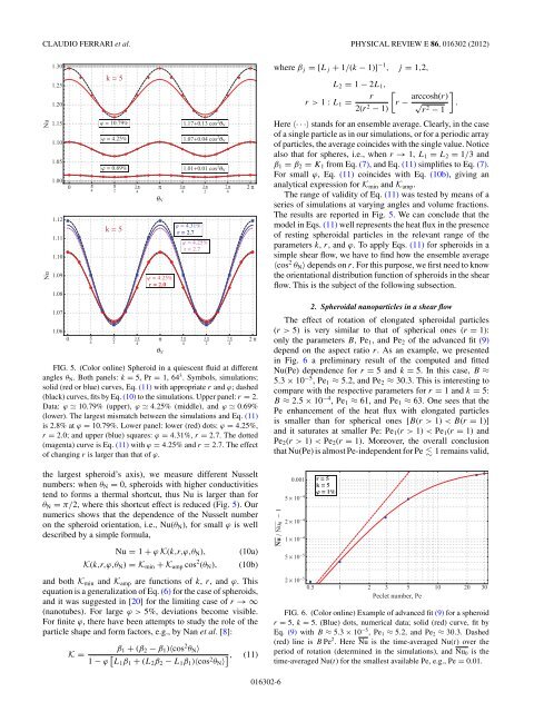
FIG. 5. (Color online) Spheroid in a quiescent fluid at different
angles θN. Bothpanels:k = 5, Pr = 1, 64 3 . Symbols, simulations;
solid (red or blue) curves, Eq. (11) with appropriate r and ϕ; dashed
(black) curves, fits by Eq. (10) to the simulations. Upper panel: r = 2.
Data: ϕ 10.79% (upper), ϕ 4.25% (middle), and ϕ 0.69%
(lower). The largest mismatch between the simulations and Eq. (11)
is 2.8% at ϕ = 10.79%. Lower panel: lower (red) dots: ϕ = 4.25%,
r = 2.0; and upper (blue) squares: ϕ = 4.31%, r = 2.7. The dotted
(magenta) curve is Eq. (11) with ϕ = 4.25% and r = 2.7. The effect
of changing r is larger than that of ϕ.
the largest spheroid’s axis), we measure different Nusselt
numbers: when θN = 0, spheroids with higher conductivities
tend to forms a thermal shortcut, thus Nu is larger than for
θN = π/2, where this shortcut effect is reduced (Fig. 5). Our
numerics shows that the dependence of the Nusselt number
on the spheroid orientation, i.e., Nu(θN), for small ϕ is well
described by a simple formula,
5 π
4
3 π
2
3 π
2
7 π
4
7 π
4
2 π
2 π
Nu = 1 + ϕ K(k,r,ϕ,θN), (10a)
K(k,r,ϕ,θN) = Kmin + Kamp cos 2 (θN), (10b)
and both Kmin and Kamp are functions of k, r, and ϕ. This
equation is a generalization of Eq. (6) for the case of spheroids,
and it was suggested in [20] for the limiting case of r →∞
(nanotubes). For large ϕ>5%, deviations become visible.
For finite ϕ, there have been attempts to study the role of the
particle shape and form factors, e.g., by Nan et al. [8]:
β1 + (β2 − β1)〈cos
K =
2θN〉 1 − ϕ L1β1 + (L2β2 − L1β1)〈cos2 , (11)
θN〉
where βj = [Lj + 1/(k − 1)] −1 , j = 1,2,
r>1:L1 =
L2 = 1 − 2L1,
r
2(r 2 − 1)
r − arccosh(r)
√ .
r2 − 1
Here 〈···〉stands for an ensemble average. Clearly, in the case
of a single particle as in our simulations, or for a periodic array
of particles, the average coincides with the single value. Notice
also that for spheres, i.e., when r → 1, L1 = L2 = 1/3 and
β1 = β2 = K1 from Eq. (7), and Eq. (11) simplifies to Eq. (7).
For small ϕ, Eq.(11) coincides with Eq. (10b), givingan
analytical expression for Kmin and Kamp.
The range of validity of Eq. (11) was tested by means of a
series of simulations at varying angles and volume fractions.
The results are reported in Fig. 5. We can conclude that the
model in Eqs. (11) well represents the heat flux in the presence
of resting spheroidal particles in the relevant range of the
parameters k, r, and ϕ. To apply Eqs. (11) for spheroids in a
simple shear flow, we have to find how the ensemble average
〈cos 2 θN〉 depends on r. For this purpose, we first need to know
the orientational distribution function of spheroids in the shear
flow. This is the subject of the following subsection.
2. Spheroidal nanoparticles in a shear flow
The effect of rotation of elongated spheroidal particles
(r >5) is very similar to that of spherical ones (r = 1):
only the parameters B, Pe1, and Pe2 of the advanced fit (9)
depend on the aspect ratio r. As an example, we presented
in Fig. 6 a preliminary result of the computed and fitted
Nu(Pe) dependence for r = 5 and k = 5. In this case, B ≈
5.3 × 10−5 ,Pe1≈ 5.2, and Pe2 ≈ 30.3. This is interesting to
compare with the respective parameters for r = 1 and k = 5:
B ≈ 2.5 × 10−4 ,Pe1≈61, and Pe1 ≈ 63. One sees that the
Pe enhancement of the heat flux with elongated particles
is smaller than for spherical ones [B(r >1) 1) < Pe1(r = 1) and
Pe2(r >1) < Pe2(r = 1). Moreover, the overall conclusion
that Nu(Pe) is almost Pe-independent for Pe 1 remains valid,
Nu Nu 0 1
016302-6
0.001
5 10 4
2 10 4
1 10 4
5 10 5
2 10 5
r 5
k 5
1
0.5 1 2 3 5 10 20 30
Peclet number, Pe
FIG. 6. (Color online) Example of advanced fit (9) for a spheroid
r = 5, k = 5. (Blue) dots, numerical data; solid (red) curve, fit by
Eq. (9) with B ≈ 5.3 × 10 −5 ,Pe1 ≈ 5.2, and Pe2 ≈ 30.3. Dashed
(red) line is B Pe 2 . Here Nu is the time-averaged Nu(t) over the
period of rotation (determined in the simulations), and Nu0 is the
time-averaged Nu(t) for the smallest available Pe, e.g., Pe = 0.01.